Adaptive estimation in the nonparametric random coefficients binary choice model by needlet thresholding

Abstract

In the random coefficients binary choice model, a binary variable equals 1 iff an index $X^{\top}\beta$ is positive. The vectors $X$ and $\beta$ are independent and belong to the sphere $\mathbb{S}^{d-1}$ in $\mathbb{R}^{d}$. We prove lower bounds on the minimax risk for estimation of the density $f_{\beta}$ over Besov bodies where the loss is a power of the ${\rm L}^{p}(\mathbb{S}^{d-1})$ norm for $1\leq p\leq\infty$. We show that a hard thresholding estimator based on a needlet expansion with data-driven thresholds achieves these lower bounds up to logarithmic factors.

1 Introduction

Discrete choice models (see, e.g., [21]) have applications in many areas ranging from planning of public transportation, economics of industrial organizations, evaluation of public policies, among others. This paper considers the binary choice model. There, agents (consumer, firm, country, etc.) choose between two exclusive alternatives 1 or -1 (e.g., buying a good or not) the one that yields the highest utility. The utility that an agent $i$ gets from choosing alternative -1 (resp. from choosing 1) is assumed to have the form

$$u_{-1,i}=z_{-1,i}^{\top}\gamma_{i}+\epsilon_{-1,i}\quad\mathrm{(resp.\ }u_{1,i}=z_{1,i}^{\top}\gamma_{i}+\epsilon_{1,i}),$$ (1)

where $z_{-1,i}$ (resp. $z_{1,i}$) is a vector of $d-1$ characteristics of alternative -1 (resp. 1) for agent $i$, $d\geq 2$, $\gamma_{i}$ are preferences of agent $i$ for the characteristics, and $\epsilon_{-1,i}$ and $\epsilon_{1,i}$ absorb both the usual error terms and constants. In (1), the preferences are allowed to vary across individuals; namely, they are heterogeneous. This translates into a vector of coefficients $\gamma$ indexed by $i$ that we assume random. The characteristics of the alternatives are indexed by the agents, for example they can be characteristics of two goods that a consumer has to choose upon interacted with individual characteristics like age or distance. We assume that the random coefficients and errors are independent from the characteristics. The statistician observes a sample of characteristics and choices for agents $i=1,\dots,n$, but $\gamma_{i}$, $u_{1,i}$, and $u_{-1,i}$ are not observed. Observing the choices corresponds to observing the sign $y_{i}$ of the net utility $u_{1,i}-u_{-1,i}$. Indeed, agent $i$ prefers 1 ($y_{i}=1$) if and only if the net utility for 1 is positive, i.e.,

$$u_{1,i}-u_{-1,i}=\epsilon_{1,i}-\epsilon_{-1,i}+(z_{1,i}-z_{-1,i})^{\top}\gamma_{i}>0,$$ (2)

and prefers -1 ($y_{i}=-1$) when

$$u_{1,i}-u_{-1,i}<0.$$

We assume that the probability that $\left|(\epsilon_{1,i}-\epsilon_{-1,i},\gamma_{i}^{\top})^{\top}\right|$ is the 0 and thus that agent $i$ is indifferent (i.e., $u_{1,i}-u_{-1,i}=0$) on a set of 0 probability. Hence, the linear random coefficients binary choice model is

$$y_{i}={\rm sign}\left(x_{i}^{\top}\beta_{i}\right),$$ (3)

where, for a real number $a$, ${\rm sign}(a)$ is 1 if $a>0$, -1 if $a<0$, and is 0 if $a=0$,

$$x_{i} =(1,(z_{1,i}-z_{-1,i})^{\top})^{\top}/\left|(1,(z_{1,i}-z_{-1,i})^{\top})^{\top}\right|,$$

$$\beta_{i} =(\epsilon_{1,i}-\epsilon_{-1,i},\gamma_{i}^{\top})^{\top}/\left|(\epsilon_{1,i}-\epsilon_{-1,i},\gamma_{i}^{\top})^{\top}\right|,$$

and $|\cdot|$ is the Euclidean norm in ${\mathbb{R}}^{d}$. Like in [3, 4, 10, 13] among others, we consider a nonparametric specification of the joint distribution of $\beta$ and this model is more general than the Logit, Probit, and Mixed-Logit models. Note that it is important to avoid restricting the dependence between the coordinates of $(\epsilon_{1}-\epsilon_{-1},\gamma^{\top})$ since they can be functions of a deep heterogeneity parameter (e.g., the type of a consumer).

We denote by $Y$, $Z_{1}$, $Z_{-1}$, $X$, $\epsilon_{1}$, $\epsilon_{-1}$, $\gamma$, and $\beta$ the population quantities corresponding to the lower cases letters indexed by $i$. The random vectors $X$ and $\beta$ are elements of the unit sphere ${\mathbb{S}}^{d-1}$ of ${\mathbb{R}}^{d}$. For the main results of this paper we maintain the following restrictions on the distribution of $(\beta^{\top},X^{\top})^{\top}$.

Assumption 1

1. $X$ and $\beta$ are independent,

2. $X$ and $\beta$ have densities $f_{X}$ and $f_{\beta}$ with respect to the spherical measure $\sigma$.

Assumption 2

1. $f_{\beta}(x)f_{\beta}(-x)=0$ for a.e. $x$ in ${\mathbb{S}}^{d-1}$,

2. The support of $X$, denoted by ${\rm supp}(f_{X})$, is $H^{+}=\{x\in{\mathbb{S}}^{d-1}:\ x_{1}\geq 0\}$,

3. $f_{X}$ is known and we have $A_{X}\mathrel{\stackrel{{\scriptstyle\makebox[0.0pt]{\mbox{\tiny def}}}}{{=}}}\|f_{X}\|_{{\rm L}^{\infty}(H^{+})}<\infty$ and $B_{X}\mathrel{\stackrel{{\scriptstyle\makebox[0.0pt]{\mbox{\tiny def}}}}{{=}}}\|1/f_{X}\|_{{\rm L}^{\infty}(H^{+})}<\infty$.

Under Assumption 1, $f_{\beta}$ is solution of the ill-posed inverse problem: for a.e. $x\in H^{+}$

$$\mathbb{E}[Y|X=x]=\int_{{\mathbb{S}}^{d-1}}{\rm sign}\left(x^{\top}y\right)f_{\beta}(y)d\sigma(y)\mathrel{\stackrel{{\scriptstyle\makebox[0.0pt]{\mbox{\tiny def}}}}{{=}}}\mathcal{K}f_{\beta}(x).$$ (4)

The operator $\mathcal{K}$ in (4) is a convolution on ${\mathbb{S}}^{d-1}$. Estimation of $f_{\beta}$ in (4) is thus related to statistical deconvolution on ${\mathbb{S}}^{d-1}$ (see, e.g., [12, 16, 19]). However, the left-hand side of (4) is not a density but a regression function where the regressors are random. The identification issue in this model stems from the fact that: (1) the distribution of the observed data only characterizes $\mathcal{K}f_{\beta}$ on ${\rm supp}(f_{X})$ which is a proper subset of ${\mathbb{S}}^{d-1}$ and (2) due to the ${\rm sign}$ function $\mathcal{K}$ has an infinite dimensional null space. The support of $X$ can only be as large as $H^{+}$ because the first coordinate of $X$ is positive. This is because we allow for the term $\epsilon_{1,i}-\epsilon_{-1,i}$ in (2).

A simple estimator for the density of $\beta$ in this model is given in [10]. There, rates of convergence for the ${\rm L}^{p}$-losses for $1\leq p\leq\infty$ over Sobolev ellipsoïds based on the same ${\rm L}^{p}$ space (as well as confidence intervals for the value of the density at a point, treatment of endogenous regressors, and of models where some coefficients are nonrandom) are obtained under similar assumptions for choices of the smoothing parameters which depend on unknown parameters of the Sobolev ellipsoïds. It is assumed in [10] that the support of $\beta$ lies in an (unknown) hemisphere, namely, that there exists $n$ (unknown) in ${\mathbb{S}}^{d-1}$ such that $\mathbb{P}(n^{\top}\beta>0)=1$. This assumption first appeared in [13] and is stronger than (A2.1). It implies that for some difference of the characteristics, or taking a limit of these, everyone chooses the same alternative. In contrast, (A2.1) is much less restrictive and does not imply "unselected samples". However, everything in [10] also holds under (A2.1). Assumption (A2.2) requires that the support of $Z_{1}-Z_{-1}$ is ${\mathbb{R}}^{d}$ and is also made in [10, 13]. [9] allows for continuous regressors which support is a proper subset at the expense of assuming some form of unselected samples and relying on integrability assumptions involving $f_{\beta}$It is possible to obtain identification of $f_{\beta}$ when we relax (A2.2) and the requirement that $f_{X}$ exists (see (A1.2)). This is done in [8]. The estimation in this case is the subject of future work. (A2.3) strengthens (A2.2) and is used to obtain rates of convergence. It could be viewed as an assumption on the tails of $X$. It is relaxed in [10] and in this paper at the end of Section 5. Note as well that Assumption (A1.2) allows for one nonrandom coefficient in the original scale and that when there are more than two, one should proceed as in Section 5.2 in [10] with the estimator developed in this paper.

In this paper, we show that the estimator in [10] can be written as a plug-in of a linear needlet estimator. Needlets are a class of linear combinations of spherical harmonics which form a tight frame of localized functions on spheres (see [25]). Hard-thresholding of series estimators based on needlets have been successfully used in statistics for estimation of functions defined on spheres (see [2] for densities, [24] for regression functions, and [17, 18, 19] for some inverse problems) or compact manifolds (see [15]). This paper proves lower bounds on the minimax risk when the degree of integrability in the loss - specified by the statistician - can differ from the degree of integrability of the Besov body containing the unknown $f_{\beta}$, giving rise to sparse and dense regimes. The lower bounds correspond, up to logarithmic factors, to the upper bounds in [10] over Sobolev ellipsoïds and matching degrees of integrability. This paper proposes to replace the linear needlet estimator in [10] by a nonlinear estimator based on hard-thresholding with data-driven thresholds and use the same plug-in strategy as in [10]. The upper bounds on the risk of the estimator also correspond to the lower bounds up to a logarithmic factor, but over all Besov bodies, including nonmatching degrees of integrability. Both the upper and lower bounds are also given for the sup-norm loss. The data-driven thresholds are similar in spirit to [5] for density estimation using the Dantzig selector (see also [6, 24] for other local thresholding procedures over the sphere), they are based on sharp concentration inequalities and make the implementation of the estimator feasible as it is independent of features of the unknown density. Proofs are given in the appendix.

2 Preliminaries

We use the notation $x\wedge y$ and $x\vee y$ for the minimum and the maximum between $x$ and $y$. We write $x\lesssim y$ when there exists $c$ such that $x\leq cy$, $x\gtrsim y$ when there exists $c$ such that $x\geq cy$, and $x\simeq y$ when $x\lesssim y$ and $x\gtrsim y$. We denote by $|A|$ and $\mathbf{1}_{A}$ the cardinal and indicator of the set $A$, by $\mathbb{N}$ the nonnegative integers, by $\mathbb{N}^{*}$ the positive integers, by a.e. almost every, and by a.s. almost surely. We denote for $1\leq p\leq\infty$ by $\|\cdot\|_{\ell^{p}}$ the $\ell^{p}$-norm of a vector, by $\|\cdot\|_{p}$ the usual norm on the space ${\rm L}^{p}({\mathbb{S}}^{d-1})$ of $p$ integrable real-valued functions with respect to the spherical measure $\sigma$. We write ${\rm L}^{p}_{{\rm odd}}({\mathbb{S}}^{d-1})$ (resp. ${\rm L}^{p}_{{\rm even}}({\mathbb{S}}^{d-1})$) the closure in ${\rm L}^{p}({\mathbb{S}}^{d-1})$ of continuous functions on ${\mathbb{S}}^{d-1}$ which are odd (i.e., for every $x\in{\mathbb{S}}^{d-1}$, $f(-x)=-f(x)$) (resp. even). Every $f\in{\rm L}^{p}({\mathbb{S}}^{d-1})$ can be uniquely decomposed as the sum of an odd and even function $f^{-}$ and $f^{+}$ in ${\rm L}^{p}({\mathbb{S}}^{d-1})$. The space ${{\rm L}^{2}}({\mathbb{S}}^{d-1})$ is a Hilbert space with the scalar product $\langle\ ,\ \rangle$ derived from the norm, there $f^{-}$ and $f^{+}$ are orthogonal. $\mathcal{D}$ is the set of densities and, as it will become clear after Proposition 5, $\nu(d)=d/2$ is the degree of ill-posedness of the inverse problem.

2.1 Harmonic analysis

The basic element is the orthogonal decomposition ${{\rm L}^{2}}({\mathbb{S}}^{d-1})=\bigoplus_{k\in{\mathbb{N}}}H^{k,d}$, where $H^{k,d}$ are the eigenspaces of the Laplacian $\Delta$ on ${\mathbb{S}}^{d-1}$, corresponding to the eigenvalues $-\zeta_{k,d}$, given by $\zeta_{k,d}\mathrel{\stackrel{{\scriptstyle\makebox[0.0pt]{\mbox{\tiny def}}}}{{=}}}k(k+d-2)$, of dimension $L(k,d)\mathrel{\stackrel{{\scriptstyle\makebox[0.0pt]{\mbox{\tiny def}}}}{{=}}}(2k+d-2)(k+d-2)!/(k!(d-2)!(k+d-2))$. The space $H^{k,d}$ is spanned by an orthonormal basis $\left(h_{k,l}\right)_{l=1}^{L(k,d)}$ and $H^{0,d}$ by $1$. We also have ${\rm L}^{2}_{\text{ odd}}({\mathbb{S}}^{d-1})=\bigoplus_{p\in{\mathbb{N}}}H^{2p+1,d}$ and ${\rm L}^{2}_{\text{ even}}({\mathbb{S}}^{d-1})=\bigoplus_{p\in{\mathbb{N}}}H^{2p,d}$. The projector $L_{k,d}$ onto $H^{k,d}$ is the operator with kernel

$$L_{k,d}(x,y)=\sum_{l=1}^{L(k,d)}h_{k,l}(x)h_{k,l}(y)=\frac{L(k,d)}{\sigma({\mathbb{S}}^{d-1})P_{k}^{\mu(d)}(1)}P_{k}^{\mu(d)}\left(x^{\top}y\right),$$ (5)

where $\mu(d)=(d-1)/2$, the surface of ${\mathbb{S}}^{d-1}$ is $\sigma({\mathbb{S}}^{d-1})=2\pi^{d/2}/\Gamma(d/2)$, and $C_{k}^{\mu}$ are the Gegenbauer polynomials. The Gegenbauer polynomials, defined for $\mu>-1/2$, are orthogonal in the space of square integrable functions on $[-1,1]$ with measure $(1-t^{2})^{\mu-1/2}dt$. We have $P_{0}^{\mu}(t)=1$, $P_{1}^{\mu}(t)=2\mu t$ for $\mu\neq 0$, $P_{1}^{0}(t)=2t$, and for every $k\in\mathbb{N}$

$$(k+2)P_{k+2}^{\mu}(t)=2(\mu+k+1)tP_{k+1}^{\mu}(t)-(2\mu+k)P_{k}^{\mu}(t).$$ (6)

Clearly, for $f\in{\rm L}^{2}({\mathbb{S}}^{d-1})$, we have $f=\sum_{k=0}^{\infty}L_{k,d}f$ and, due to (5),

$$\forall x\in{\mathbb{S}}^{d-1},\ \|L_{k,d}(x,\cdot)\|_{2}^{2}=\sum_{l=1}^{L(k,d)}|h_{k,l}(x)|^{2}=\frac{L(k,d)}{\sigma({\mathbb{S}}^{d-1})}.$$ (7)

Powers $\left(-\Delta\right)^{s}f$ for $s\in{\mathbb{R}}$ and $f$ in a Banach space $E_{1}$ are defined in a Banach space $E_{2}$ when $L_{k,d}f$ is defined in $E_{2}$ and $\left(-\Delta\right)^{s}f\mathrel{\stackrel{{\scriptstyle\makebox[0.0pt]{\mbox{\tiny def}}}}{{=}}}\sum_{k=0}^{\infty}\zeta_{k,d}^{s}L_{k,d}f$ converges in $E_{2}$. The best approximation in ${\rm L}^{r}({\mathbb{S}}^{d-1})$ of a function $f$ by harmonics of degree less or equal to $m$ is

$$E_{m}(f)_{r}=\inf_{P\in\bigoplus_{k=0}^{m}H^{k,d}}\left\|f-P\right\|_{r}.$$

Definition 3

For $s>0$ and $1\leq r\leq\infty$, $f$ belongs to the Sobolev space ${\rm W}^{s}_{r}({\mathbb{S}}^{d-1})$ if

$$\|f\|_{r,s}=\|f\|_{r}+\left\|\left(-\Delta\right)^{s/2}f\right\|_{r}<\infty.$$

We denote by ${\rm W}_{r\ {\rm odd}}^{s}({\mathbb{S}}^{d-1})$ the restriction of ${\rm W}_{r}^{s}({\mathbb{S}}^{d-1})$ to odd functions.

Definition 4

For $s>0$, $1\leq r\leq\infty$, and $0<q\leq\infty$, $f$ belongs to the Besov space $B^{s}_{r,q}({\mathbb{S}}^{d-1})$ if

$$\left\|f\right\|^{A}_{B^{s}_{r,q}}=\|f\|_{r}+\left\|\left(2^{js}E_{2^{j}}(f)_{r}\right)_{j\in{\mathbb{N}}}\right\|_{\ell^{q}}<\infty.$$

2.2 The operator

Proposition 5

The operator $\mathcal{K}$ satisfies the following properties:

1. For every $f\in{\rm L}^{1}({\mathbb{S}}^{d-1})$, $\mathcal{K}f=\mathcal{K}(f^{-})$,

2. If $\mathcal{K}f=\mathcal{K}g$ with $f,g\in{\rm L}^{1}_{{\rm odd}}({\mathbb{S}}^{d-1})$ then $g=f$,

3. For every $1\leq r\leq\infty$,

   $${\rm W}^{\nu(d)+|1/r-1/2|(d-2)}_{r\ {\rm odd}}({\mathbb{S}}^{d-1})\subseteq\mathcal{K}({\rm L}^{r}_{{\rm odd}}({\mathbb{S}}^{d-1}))\subseteq{\rm W}^{\nu(d)-|1/r-1/2|(d-2)}_{r\ {\rm odd}}({\mathbb{S}}^{d-1}),$$

   where the exponents $\nu(d)\pm|1/r-1/2|(d-2)$ cannot be improved,

4. For every $1\leq r\leq\infty$, there exists $B(d,r)$ such that

   $$\forall K\in{\mathbb{N}},\ \forall P\in\bigoplus_{\begin{subarray}{c}k=0\\ k\ {\rm odd}\end{subarray}}^{K}H^{k,d},\ \|\mathcal{K}^{-1}P\|_{r}\leq B(d,r)K^{\nu(d)}\|P\|_{r}.$$ (8)

Moreover, $\mathcal{K}$ is a self-adjoint and compact operator on ${\rm L}^{2}({\mathbb{S}}^{d-1})$ with null space ${\rm L}_{{\rm even}}^{2}({\mathbb{S}}^{d-1})$, nonzero eigenvalues $(\lambda_{2p+1,d})_{p\in{\mathbb{N}}}$ corresponding to the eigenspaces $H^{2p+1,d}$ for $p\in\mathbb{N}$

$$\lambda_{1,d}=\frac{2|\mathbb{S}^{d-2}|}{d-1},\ \forall p\in\mathbb{N}^{*}\ \lambda_{2p+1,d}=\frac{2(-1)^{p}|\mathbb{S}^{d-2}|1\cdot 3\cdots(2p-1)}{(d-1)(d+1)\cdots(d+2p-1)}.$$

For every $d\in{\mathbb{N}}\setminus\{1\}$, for every $p\in{\mathbb{N}}$, there exists $c_{\lambda}(d),C_{\lambda}(d)>0$ such that

$$c_{\lambda}^{-1}(d)p^{-\nu(d)}\leq\left|\lambda_{2p+1,d}\right|\leq C_{\lambda}(d)p^{-\nu(d)}.$$ (9)

$\mathcal{K}$ is a homeomorphism between ${\rm L}_{{\rm odd}}^{2}({\mathbb{S}}^{d-1})$ and ${\rm W}_{2\ {\rm odd}}^{\nu(d)}({\mathbb{S}}^{d-1})$.

The fact that $\nu(d)$ is the degree of ill-posedness of the inverse problem follows from (P1.4) and what follows, in particular (9).

Proposition 5 implies that every $R\in{\rm W}_{2\ \text{ odd}}^{\nu(d)}({\mathbb{S}}^{d-1})$ has a unique inverse given by

$$\mathcal{K}^{-1}\left(R\right)=\sum_{k\ {\rm odd}}\frac{1}{\lambda_{k,d}}L_{k,d}\left(R\right)=\sum_{k\ {\rm odd}}\frac{1}{\lambda_{k,d}}\sum_{l=1}^{L(k,d)}\langle R,h_{k,l}\rangle h_{k,l}.$$ (10)

2.3 Needlets

Smoothed projection operators (see [10]) have good approximation properties in all ${\rm L}^{p}({\mathbb{S}}^{d-1})$ spaces and are uniformly bounded from ${\rm L}^{p}({\mathbb{S}}^{d-1})$ to ${\rm L}^{p}({\mathbb{S}}^{d-1})$. One such operator, the delayed means, is the integral operator with kernel

$$K^{a,J}(x,y)\mathrel{\stackrel{{\scriptstyle\makebox[0.0pt]{\mbox{\tiny def}}}}{{=}}}\sum_{k=0}^{\infty}a\left(\frac{k}{2^{J}}\right)L_{k,d}(x,y),$$ (11)

where $J$ is an integer, $a$ is a ${\rm C}^{\infty}$ and decreasing function on $[0,\infty)$ supported on $[0,2]$ such that, for every $0\leq t\leq 2$, $0\leq a(t)\leq 1$ and, for every $0\leq t\leq 1$, $a(t)=1$. The delayed means operator exhibits nearly exponential localization (see Theorem 2.2 in [25]) and is a building block for the construction of needlets.

Define $b$ such that $b^{2}(t)=a\left(t\right)-a(2t)$ for $t\geq 0$. It is nonzero only when $1/2\leq t\leq 2$, satisfies $b^{2}(t)+b^{2}(2t)=1$ for $1/2\leq t\leq 1$ and thus for every $t\geq 1$, $\sum_{j=0}^{\infty}b^{2}\left(\frac{t}{2^{j}}\right)=1$, also $b^{2}(t)=a(t)$ for $1\leq t\leq 2$. Take $a$ such that $b$ is bounded away from 0 on $3/5\leq t\leq 5/3$.

The second ingredient for the construction of needlets is a quadrature formula (Corollary 2.9 of [25]) with positive weights $\left(\omega(j,\xi)^{2}\right)_{\xi\in\Xi_{j}}$ and nodes $\xi\in\Xi_{j}$ which integrates functions in $\bigoplus_{k=0}^{2^{j}}H^{k,d}$ and satisfy, for a constant $C_{\Xi}$ which depends on $d$,

$$\forall j\in{\mathbb{N}},\ \forall\xi\in\Xi_{j},\quad C_{\Xi}^{-1}2^{j(d-1)}\leq|\Xi_{j}|\leq C_{\Xi}2^{j(d-1)}$$

$$C_{\Xi}^{-1}2^{-j(d-1)/2}\leq\omega(j,\xi)\leq C_{\Xi}2^{-j(d-1)/2}.$$

Needlets are defined as

$$\psi_{j,\xi}(x) \mathrel{\stackrel{{\scriptstyle\makebox[0.0pt]{\mbox{\tiny def}}}}{{=}}}\omega(j,\xi)\sum_{k=0}^{\infty}b\left(\frac{k}{2^{j-1}}\right)L_{k,d}(\xi,x)\quad{\rm if}\ j\in{\mathbb{N}},\ \xi\in\Xi_{j},$$ (12)

$$\psi_{0,\xi}(x) \mathrel{\stackrel{{\scriptstyle\makebox[0.0pt]{\mbox{\tiny def}}}}{{=}}}L_{0,d}(\xi,x).$$ (13)

For $j=0$, $\psi_{0,\xi}(x)$ is constant and $\Xi_{0}$ is a singleton.

The ${\rm L}^{p}$-norms of the needlets satisfy, for a constant $C_{p}$ that can depend on $d$,

$$\forall j\in{\mathbb{N}},\ \forall\xi\in\Xi_{j},\ C_{p}^{-1}2^{j(d-1)(1/2-1/p)}\leq\|\psi_{j,\xi}\|_{p}\leq C_{p}2^{j(d-1)(1/2-1/p)}.$$ (14)

If $f\in{\rm L}^{p}({\mathbb{S}}^{d-1})$ for $1\leq p\leq\infty$, then $f=\sum_{j=0}^{\infty}\sum_{\xi\in\Xi_{j}}\langle f,\psi_{j,\xi}\rangle\psi_{j,\xi}$. The needlets form a tight frame, with unitary tightness constant, this means that for $f\in{\rm L}^{2}({\mathbb{S}}^{d-1})$

$$\|f\|_{2}^{2}=\sum_{j=0}^{\infty}\sum_{\xi\in\Xi_{j}}\left|\langle f,\psi_{j,\xi}\rangle\right|^{2}.$$

Needlets do not form a basis and there is redundancy. Lemma 6 (see [2]) relates ${\rm L}^{p}({\mathbb{S}}^{d-1})$ norms at level $j$ to $\ell^{p}$ norms of needlet coefficients. Constants may depend on $d$.

Lemma 6

1. For every $1\leq p\leq\infty$, there exists a constant $C^{\prime}_{p}$ such that for every $j\in{\mathbb{N}}$ and $(\beta_{\xi})_{\xi\in\Xi_{j}}\in{\mathbb{R}}^{\Xi_{j}}$

   $$\left\|\sum_{\xi\in\Xi_{j}}\beta_{\xi}\psi_{j,\xi}\right\|_{p}\leq C^{\prime}_{p}2^{j(d-1)(1/2-1/p)}\left\|\left(\beta_{\xi}\right)_{\xi\in\Xi_{j}}\right\|_{\ell^{p}},$$ (15)

2. There exists constants $c_{A}$ and $c_{p,A}$ and sets $A_{j}\subset\Xi_{j}$ with $|A_{j}|\geq c_{A}2^{j(d-1)}$ for $j\in{\mathbb{N}}$ such that for every $1\leq p\leq\infty$, $j\in{\mathbb{N}}$, and $(\beta_{\xi})_{\xi\in A_{j}}\in{\mathbb{R}}^{A_{j}}$,

   $$\left\|\sum_{\xi\in A_{j}}\beta_{\xi}\psi_{j,\xi}\right\|_{p}\geq c_{p,A}2^{j(d-1)(1/2-1/p)}\left\|\left(\beta_{\xi}\right)_{\xi\in A_{j}}\right\|_{\ell^{p}},$$ (16)

3. For every $1\leq p\leq\infty$, there exists a constant $C^{\prime\prime}_{p}$ such that for every $j\in{\mathbb{N}}$

   $$\left(\sum_{\xi\in\Xi_{j}}|\langle f,\psi_{j,\xi}\rangle|^{p}\right)^{1/p}2^{j(d-1)(1/2-1/p)}\leq C^{\prime\prime}_{p}\|f\|_{p}.$$ (17)

Needlets are such that (see [25]), for all function $a$ in the definition of the smoothed projection operators, the norm $\left\|\cdot\right\|^{A}_{B^{s}_{r,q}}$ defining the Besov spaces is equivalent to

$$\left\|f\right\|_{B^{s}_{r,q}}=\left\|\left(2^{j(s+(d-1)(1/2-1/r))}\left\|\left(\langle f,\psi_{j,\xi}\rangle\right)_{\xi\in\Xi_{j}}\right\|_{\ell^{r}}\right)_{j\in{\mathbb{N}}}\right\|_{\ell^{q}}.$$

The ball of radius $M$ for this norm is denoted by $B^{s}_{r,q}(M)$.

Recall the following consequence of the proof of the continuous embeddings in [2].

Lemma 7

1. If $p\leq r\leq\infty$, then we have $B^{s}_{r,q}(M)\subseteq B^{s}_{p,q}(C_{\Xi}^{1/p-1/r}M)$,

2. If $s>(d-1)(1/r-1/p)$ and $r\leq p\leq\infty$, then we have $B^{s}_{r,q}(M)\subseteq B^{s-(d-1)(1/r-1/p)}_{p,q}(M)$,

3. If $f\in B^{s}_{r,q}(M)$ and $\left(\beta_{j,\xi}\right)_{\xi\in\Xi_{j},j\in{\mathbb{N}}}$ are its needlet coefficients, then there exists $(D_{j})_{j\in{\mathbb{N}}}\in{\mathbb{R}}^{{\mathbb{N}}}$ such that $\|(D_{j})_{j\in{\mathbb{N}}}\|_{\ell^{q}}\leq M$ and

   $$\forall z\geq 1,\ \forall j\in{\mathbb{N}},\ \sum_{\xi\in\Xi_{j}}|\beta_{j,\xi}|^{z}\leq C_{\Xi}^{1-(z\wedge r)/r}D_{j}^{z}2^{-jz(s+(d-1)(1/2-1/(z\wedge r)))}.$$ (18)

Finally recall that, when $f\in B^{s}_{r,q}$ with $s>(d-1)/r$, then $f$ is continuous.

3 Identification of $f_{\beta}$

Let us present the arguments for the identification of $f_{\beta}$. Proposition 5 (P1.1) implies that $\mathcal{K}f_{\beta}=\mathcal{K}f_{\beta}^{-}$ is odd. Thus under (A2.2) we can define the odd function $R$ as

$$R(x)=\left\{\begin{array}[]{ll}\mathbb{E}[Y|X=x]&\mbox{for\ a.e.}\ x\in H^{+}\\ -\mathbb{E}[Y|X=-x]&\mbox{for\ a.e.}\ x\in-H^{+}\\ \end{array}\right.$$ (19)

and we have, for a.e. $x\in{\mathbb{S}}^{d-1}$, $R(x)=\mathcal{K}f_{\beta}^{-}(x)$. Uniqueness of $f_{\beta}^{-}$ follows from (P1.2). Using, for a.e. $x\in{\mathbb{S}}^{d-1}$ $f_{\beta}(x)\geq 0$ and $f_{\beta}^{-}(x)=(f_{\beta}(x)-f_{\beta}(-x))/2$, and condition (A2.1), yields that, for a.e. $x\in{\mathbb{S}}^{d-1}$, we have

$$f_{\beta}(x)=2{f_{\beta}^{-}}(x)\mathbf{1}_{{f_{\beta}^{-}}(x)>0}.$$ (20)

In this paper we normalize the vectors of random coefficients and covariates to have unit norm. Indeed, since only the sign of the net utility (2) matters for choosing between 1 and -1 and the index is linear, a scale normalization of $(\epsilon_{1}-\epsilon_{-1},\gamma^{\top})$ is in order. Let us compare with the normalization in [9]. It is based on the following assumption, which is stronger than the condition in [13], that the support of $\beta$ is a subset of some (unknown) hemisphere, which itself is stronger than (A2.1).

(H): a.s. there exists $j\in\{1,\dots,d\}$, the coordinate $\gamma_{j}$ of $\gamma$ has a sign (excluding 0).

Assumption (H) is likely to hold when $Z_{1j}$ and $Z_{-1j}$ are cost factors, since consumers dislike an increase in cost. If (H) holds we can identify for which index $j$ $\gamma_{j}$ has a sign since it amounts to the finding for which coordinate $z_{j}$ of $z$ $z_{j}\to\mathbb{E}[Y|Z_{1}-Z_{-1}=z]$ is (globally) monotone. We can identify the sign of the coefficient by assessing whether the function is increasing (positive) or decreasing (negative). If $\gamma_{j}>0$ then we normalize the vector of coefficients by dividing by $\gamma_{j}$. If $\gamma_{j}<0$ we change the sign of $Z_{1j}-Z_{-1j}$ to make it positive. A potential issue with this normalization is that if $\beta_{j}$ can take small values then estimators could differ in finite samples depending on which coefficient is used for normalization. Also, monotonicity in one regressor of the conditional mean function implies a type of weak monotonicity (in the sense used to identify treatment effects, see, e.g., [9]) at the individual level as we now explain. Assuming that $\gamma_{j}>0$, $z_{1i}-z_{-1i}=z$ for all $i=1,\dots,n$, and that we change $z_{j}$ to $z_{j}^{\prime}>z_{j}$ while leaving unchanged $(\epsilon_{1i}-\epsilon_{-1i},\gamma_{i}^{\top})$ (the characteristics of the individuals) and the other components of $z$, then some people do not change their decision and some choose alternative 1 while originally they had chosen alternative -1, but no one changes from alternative 1 to alternative -1. Monotonicity of the conditional mean function implies monotonicity for every individual. This is sometimes not a realistic model of individuals making choices. Clearly (A2.1) allows both individuals to switch from 1 to -1 and individuals to switch from -1 to 1 after similar changes in $z$ (or $x$). On the other hand, if (H) holds then (A2.2) can be relaxed and we can consider an index which is nonlinear in $X$ (cf. [9]).

4 Lower bounds

We take $1\leq p,r\leq\infty$, $0\leq q\leq\infty$, $z\geq 1$, and $s>0$, and consider the minimax risk

$$\mathcal{R}_{n}^{*}\mathrel{\stackrel{{\scriptstyle\makebox[0.0pt]{\mbox{\tiny def}}}}{{=}}}\inf_{\widehat{f_{\beta}}}\sup_{f_{\beta}\in B^{s}_{r,q}(M)\cap\mathcal{D}}\mathbb{E}\left\|\widehat{f_{\beta}}-f_{\beta}\right\|_{p}^{z},$$ (21)

where the infimum is over all estimators based on the i.i.d. sample of size $n$. The degree of integrability $r$ in the smoothness class $B^{s}_{r,q}(M)$ is allowed to differ from the degree of integrability $p$ in the loss function. We distinguish two zones for $s,r,q,d$, and $p$:
(1) the dense zone where $s\geq p\left(\nu(d)+(d-1)/2\right)\left(1/r-1/p\right)$ with the restriction $q\leq r$ if $s=p\left(\nu(d)+(d-1)/2\right)\left(1/r-1/p\right)$, where the rate involves

$$\mu_{{\rm dense}}(d,p,r,s)\mathrel{\stackrel{{\scriptstyle\makebox[0.0pt]{\mbox{\tiny def}}}}{{=}}}s/(s+\nu(d)+(d-1)/2),$$

(2) the sparse zone where $(d-1)/r<s<p\left(\nu(d)+(d-1)/2\right)\left(1/r-1/p\right)$, where the rate involves

$$\mu_{{\rm sparse}}(d,p,r,s)\mathrel{\stackrel{{\scriptstyle\makebox[0.0pt]{\mbox{\tiny def}}}}{{=}}}(s-(d-1)(1/r-1/p))/(s+\nu(d)-(d-1)(1/r-1/2)).$$

The terminology dense and sparse is justified by the following heuristic. The proofs of the lower bounds replace the infimum in (21) by a minimum over a set of functions which are difficult to estimate. The functions used to prove the lower bound in the dense zone are functions which could have many nonzero needlet coefficients for $\xi\in A_{j}$ (see Lemma 6) and a well-chosen $j$. Those used to prove the lower bound in the sparse zone only have two nonzeros. In the dense zone, the rate is the same as for the matched case when $r=p$ studied in [10].

Theorem 8

1. In the dense zone we have

   $$\mathcal{R}_{n}^{*}\geq c_{{\rm dense}}(d,M,p,r,s,z)\left(\frac{1}{\sqrt{nA_{X}}}\right)^{\mu_{{\rm dense}}(d,p,r,s)z},$$ (22)

2. In the sparse zone we have

   $$\mathcal{R}_{n}^{*}\geq c_{{\rm sparse}}(d,M,p,r,s,z)\left(\sqrt{\frac{\ln(nA_{X})}{nA_{X}}}\right)^{\mu_{{\rm sparse}}(d,p,r,s)z},$$ (23)

where the constants $c_{{\rm dense}}$ and $c_{{\rm sparse}}$ depend on $d$, $M$, $p$, $r$, $s$ and $z$.

The values of $\mu_{{\rm dense}}$ and $\mu_{{\rm sparse}}$ depend on $d$ through the dimension of ${\mathbb{S}}^{d-1}$. This is the usual curse of dimensionality in nonparametric regression or density estimation. They also depend on $d$ through the degree of ill-posedness $\nu(d)=d/2$ of the inverse problem.

5 Adaptive estimation by needlet thresholding

Consider the estimator $\widehat{f_{\beta}}=2\widehat{{f_{\beta}^{-}}}\mathbf{1}_{\widehat{{f_{\beta}^{-}}}>0}$, where $\widehat{{f_{\beta}^{-}}}$ is an estimator of ${f_{\beta}^{-}}$.

5.1 Smoothed projections and linear needlet estimators

A smoothed projection estimator of $f_{\beta}^{-}$ with kernel (11), window $a$, and $J\in{\mathbb{N}}$, is given for $x\in{\mathbb{S}}^{d-1}$ by

$$\widehat{{f_{\beta}^{-}}}^{a,J}(x)=\sum_{k\ {\rm odd}}\frac{a\left(\frac{k}{2^{J}}\right)}{\lambda_{k,d}}\widehat{L_{k,d}R}(x),$$

with the unbiased estimator of $L_{k,d}R(x)$ (see Lemma 10): $\widehat{L_{k,d}R}(x)=0$ if $k$ is even, else

$$\widehat{L_{k,d}R}(x)=\frac{2}{n}\sum_{i=1}^{n}\frac{y_{i}L_{k,d}(x_{i},x)}{f_{X}(x_{i})}.$$

Alternatively, we can estimate ${f_{\beta}^{-}}$ using the needlet frame with smoothing window $a$. The coefficients $\beta^{a}_{j,\xi}=\langle{f_{\beta}^{-}},\psi_{j,\xi}\rangle$ are such that

$$\beta^{a}_{j,\xi} =\omega(j,\xi)\sum_{k\text{ odd}}b\left(\frac{k}{2^{j-1}}\right)\langle{f_{\beta}^{-}},L_{k,d}(\xi,\cdot)\rangle$$

$$=\omega(j,\xi)\sum_{k\text{ odd}}\frac{b\left(\frac{k}{2^{j-1}}\right)}{\lambda_{k,d}}\langle L_{k,d}R,L_{k,d}(\xi,\cdot)\rangle$$

$$=\omega(j,\xi)\sum_{\begin{subarray}{c}k\text{ odd}\\ 2^{j-2}<k<2^{j}\end{subarray}}\frac{b\left(\frac{k}{2^{j-1}}\right)}{\lambda_{k,d}}L_{k,d}R(\xi).$$

Using that $a\left(\frac{k}{2^{j}}\right)=1$ for $k=0,\ldots,2^{j}$ and denoting by ${f_{\beta}^{-}}^{a,J}=\mathbb{E}\left[\widehat{{f_{\beta}^{-}}}^{a,J}\right]$, we obtain that, for $1\leq j\leq J$, $\beta^{a}_{j,\xi}=\left\langle{f_{\beta}^{-}}^{a,J},\psi_{j,\xi}\right\rangle$, which can be estimated without bias by

$$\widehat{\beta}^{a}_{j,\xi}=\omega(j,\xi)\sum_{k\text{ odd}}\frac{b\left(\frac{k}{2^{j-1}}\right)}{\lambda_{k,d}}\widehat{L_{k,d}R}(\xi)\stackrel{{\scriptstyle(\triangle_{1})}}{{=}}\left\langle\widehat{{f_{\beta}^{-}}}^{a,J},\psi_{j,\xi}\right\rangle.$$

Moreover, for $x\in{\mathbb{S}}^{d-1}$,

$$\widehat{\beta}^{a}_{j,\xi}\psi_{j,\xi}(x)=\omega(j,\xi)^{2}\left(\sum_{k\text{ odd}}\frac{b\left(\frac{k}{2^{j-1}}\right)}{\lambda_{k,d}}\widehat{L_{k,d}R}(\xi)\right)\left(\sum_{k}b\left(\frac{k}{2^{j-1}}\right)L_{k,d}(\xi,x)\right)$$

belongs to $\bigoplus_{k=0}^{2^{j}}H^{k,d}$, thus by the quadrature formula

$$\sum_{\xi\in\Xi_{j}}\widehat{\beta}^{a}_{j,\xi}\psi_{j,\xi}(x)=\sum_{k\text{ odd}}\frac{b^{2}\left(\frac{k}{2^{j-1}}\right)}{\lambda_{k,d}}\widehat{L_{k,d}R}(x).$$

This yields $\sum_{j=0}^{J}\sum_{\xi\in\Xi_{j}}\widehat{\beta}^{a}_{j,\xi}\psi_{j,\xi}=\widehat{{f_{\beta}^{-}}}^{a,J-1}$, indeed

$$\sum_{j=0}^{J}\sum_{\xi\in\Xi_{j}}\widehat{\beta}^{a}_{j,\xi}\psi_{j,\xi} =\sum_{j=1}^{J}\sum_{\xi\in\Xi_{j}}\widehat{\beta}^{a}_{j,\xi}\psi_{j,\xi}\quad\mathrm{(due\ to\ }(\triangle_{1})\ \mathrm{and\ because\ }\widehat{{f_{\beta}^{-}}}^{a,J}\ \mathrm{is\ odd)}$$

$$\stackrel{{\scriptstyle(\triangle_{2})}}{{=}}\sum_{\begin{subarray}{c}1\leq k<2^{J-1}\\ k\text{ odd}\end{subarray}}\frac{1}{\lambda_{k,d}}\widehat{L_{k,d}R}+\sum_{\begin{subarray}{c}2^{J-1}\leq k\leq 2^{J}\\ k\text{ odd}\end{subarray}}\frac{b^{2}\left(\frac{k}{2^{J-1}}\right)}{\lambda_{k,d}}\widehat{L_{k,d}R}$$

$$\stackrel{{\scriptstyle(\triangle_{3})}}{{=}}\sum_{\begin{subarray}{c}1\leq k<2^{J-1}\\ k\text{ odd}\end{subarray}}\frac{1}{\lambda_{k,d}}\widehat{L_{k,d}R}+\sum_{\begin{subarray}{c}2^{J-1}\leq k\leq 2^{J}\\ k\text{ odd}\end{subarray}}\frac{a\left(\frac{k}{2^{J-1}}\right)}{\lambda_{k,d}}\widehat{L_{k,d}R},$$

where ($\triangle_{2}$) uses that for $1/2\leq t\leq 1$, $b^{2}(t)+b^{2}(2t)=1$, while ($\triangle_{3}$) that $b^{2}(t)=a\left(t\right)$ for $1\leq t\leq 2$. Thus, the smoothed projection and needlet estimators coincide.

5.2 Nonlinear estimator with data-driven thresholds

Consider, for $\gamma\geq 1$ and $\rho_{T_{j,\xi,\gamma}}(x)=x\mathbf{1}_{|x|>T_{j,\xi,\gamma}}$, the nonlinear estimator of ${f_{\beta}^{-}}$:

$$\widehat{{f_{\beta}^{-}}}^{a,\rho}=\sum_{j=0}^{J}\sum_{\xi\in\Xi_{j}}\rho_{T_{j,\xi,\gamma}}\left(\widehat{\beta}^{a}_{j,\xi}\right)\psi_{j,\xi}.$$

It is classical that the optimal choice of $J$ for linear estimators depends on the parameters of the smoothness ellipsoid. In contrast, using a thresholded estimator allows to take $J$ large and independent of the parameters. Thresholding induces additional bias compared to linear estimators which allows to reduce the variance incurred by taking $J$ large.

The level of thresholding should depend on the size of the coefficients relative to their variance. This variance is proportional to $1/\sqrt{n}$ so that the level of the threshold does not have to depend on the smoothness of the unknown function. Instead of using a conservative upper bound on their variance, as is usually the case in estimation using wavelets, we use data-driven levels of thresholding. These provide better estimators in small samples. Lemma 14 gives a theoretical guarantee that the performance is almost as good as that of an oracle which would know the variance of the estimators of the coefficients. The data-driven thresholding rule uses that $\widehat{\beta}^{a}_{j,\xi}=\frac{1}{n}\sum_{i=1}^{n}G_{j,\xi}(x_{i},y_{i})$ with

$$G_{j,\xi}(x_{i},y_{i})\mathrel{\stackrel{{\scriptstyle\makebox[0.0pt]{\mbox{\tiny def}}}}{{=}}}\frac{2}{n}\sum_{i=1}^{n}\omega(j,\xi)\frac{y_{i}}{f_{X}(x_{i})}\sum_{k\text{ odd}}\frac{b\left(\frac{k}{2^{j-1}}\right)}{\lambda_{k,d}}L_{k,d}(x_{i},\xi).$$ (24)

Define the estimator of the variance by

$$\hat{\sigma}_{j,\xi}\mathrel{\stackrel{{\scriptstyle\makebox[0.0pt]{\mbox{\tiny def}}}}{{=}}}\sqrt{\frac{1}{n(n-1)}\sum_{i=2}^{n}\sum_{k=1}^{i-1}\left(G_{j,\xi}(x_{i},y_{i})-G_{j,\xi}(x_{k},y_{k})\right)^{2}},$$ (25)

$t_{n}=\sqrt{\log n/n}$, and the data-driven thresholds

$$T_{j,\xi,\gamma}\mathrel{\stackrel{{\scriptstyle\makebox[0.0pt]{\mbox{\tiny def}}}}{{=}}}2\sqrt{2\gamma}t_{n}\widehat{\sigma}_{j,\xi}+\frac{28}{3}M_{j,\xi}\frac{\gamma\log n}{n-1},$$

where $M_{j,\xi}$ is an upper bound on the sup-norm over $H^{+}\times\{\pm 1\}$ of $G_{j,\xi}(x,y)-\mathbb{E}\left[G_{j,\xi}(X,Y)\right]=G_{j,\xi}(x,y)-\beta^{a}_{j,\xi}$ (e.g., $2\|G_{j,\xi}\|_{\infty}$). For example, using (14) and Proposition 5, we get

$$2\|G_{j,\xi}\|_{\infty}\leq 2\left\|\mathcal{K}^{-1}\left(\psi_{j,\xi}^{-}\right)\right\|_{\infty}B_{X}\leq 2C_{\infty}B(d,\infty)2^{j(\nu(d)+(d-1)/2)}B_{X}\mathrel{\stackrel{{\scriptstyle\makebox[0.0pt]{\mbox{\tiny def}}}}{{=}}}M_{j}.$$ (26)

The second term in $T_{j,\xi,\gamma}$ controls the error in estimating the threshold.

Theorem 9

For $J$ such that $2^{J(\nu(d)+(d-1)/2)}B_{X}^{1/2}\simeq t_{n}^{-1}$, $M>0$, and $s>(d-1)/r$,

1. If $z>1$ and $\gamma>z/2+1$, we have

   $$\sup_{f_{\beta}\in B^{s}_{r,q}(M)\cap\mathcal{D}}\mathbb{E}\left\|\widehat{f_{\beta}}^{a,\rho}-f_{\beta}\right\|_{\infty}^{z}\leq\tilde{c}(d,\infty,r,s,\gamma)(\log n)^{z-1}M^{r}\left(B_{X}t_{n}\right)^{\mu_{{\rm sparse}}(d,\infty,r,s)z}.$$ (27)

2. If $p<\infty$ and $\gamma>p/2$, we have

   $$\sup_{f_{\beta}\in B^{s}_{r,q}(M)\cap\mathcal{D}}\mathbb{E}\left\|\widehat{f_{\beta}}^{a,\rho}-f_{\beta}\right\|_{p}^{p}\leq\tilde{c}(d,p,r,s,\gamma)(\log n)^{p-1}M^{\varpi}\left(B_{X}t_{n}\right)^{\mu(d,p,r,s)p},$$ (28)

   where $\mu(d,p,r,s)=\mu_{{\rm dense}}(d,p,r,s)$ and $\varpi=r$ in the dense zone, while $\mu(d,p,r,s)=\mu_{{\rm sparse}}(d,p,r,s)$ and $\varpi>p\frac{\nu(d)+(d-1)(1/2-1/p)}{s+\nu(d)-(d-1)(1/r-1/2)}$ is arbitrary in the sparse zone, and $\tilde{c}(d,p,r,s,\gamma)$ is a constant which depends on $d,p,r,s$, and $\gamma$.

The upper bounds in Theorem 9 match the lower bound in Theorem 8 up to logarithmic factors. Hence, the proposed estimator is minimax adaptive (up to the $\log$ factors).

6 Simulation study

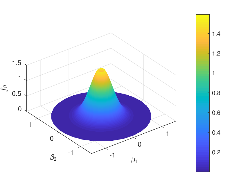
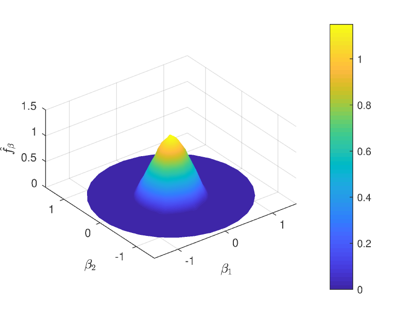
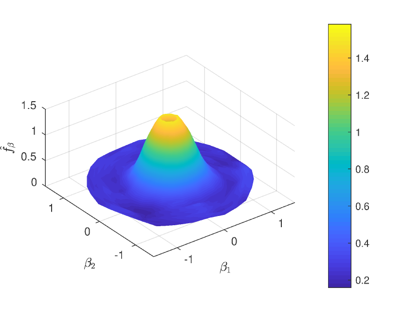
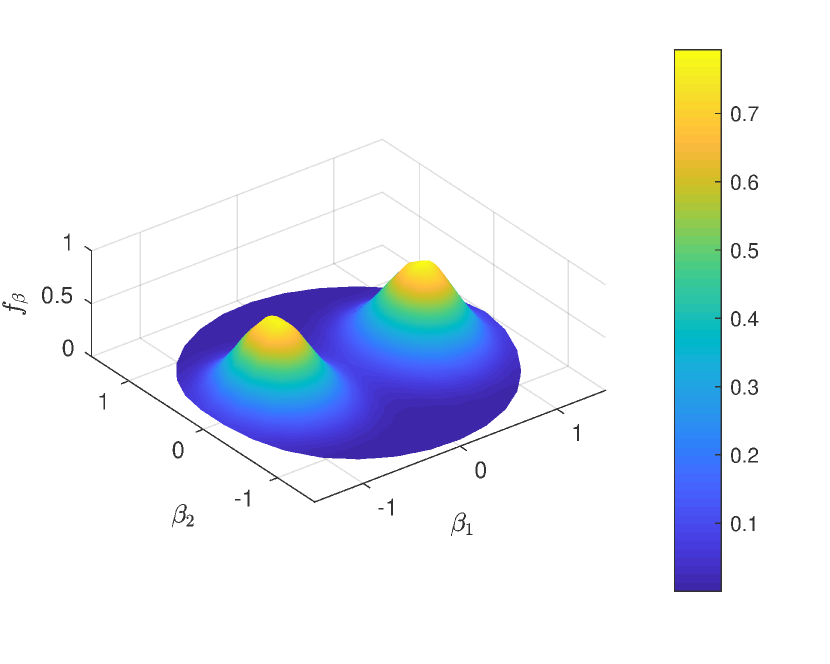
We study the performance of the estimator when $d=3$, $n=3000,5000,10000$, and $X$ is uniform on $H^{+}$. We use of the Von Mises-Fisher distribution $\mathrm{vMF}(\mu,\kappa)$ with density

$$f(\beta;\mu,\kappa)=\frac{\kappa}{4\pi\sinh\kappa}\exp\left(\kappa\mu^{\top}\beta\right)$$

with respect to $\sigma$. We take $\beta=(\tilde{\beta_{1}},\tilde{\beta_{2}},|\tilde{\beta_{3}}|)$ in the cases:

• $\tilde{\beta}$ follows a $\mathrm{vMF}(\mu,\kappa)$ distribution where $\mu=(0\ 0\ 1)^{\top}$ and $\kappa=10$.

• $\tilde{\beta}$ follows a mixture $\lambda\mathrm{vMF}(\mu_{1},\kappa)+(1-\lambda)\mathrm{vMF}(\mu_{2},\kappa),$ where $\mu_{1}=(2^{-1/2}\ 0\ 2^{-1/2})^{\top}$, $\mu_{2}=(-2^{-1/2}\ 0\ 2^{-1/2})^{\top}$, $\kappa=10$ and $\lambda=0.3$.

We use the cubature defined in spherical coordinates as a product of the Gauss-Legendre quadrature with $m$ nodes and trapezoid rule with $2m$ subdivisions (see [1]). The resulting cubature has $2m^{2}$ nodes and integrates exactly all polynomials on the sphere up to degree $2m-1$. We take the same function $a$ as in [2].

The threshold is driven by the parameter $\gamma$. The choice of $\gamma$ slightly depends on the targeted norm. Here we focus on a simultaneous control of the ${\rm L}^{1}$, $xL^{2}$, $xL^{4}$ and ${\rm L}^{\infty}$ norm. According to our analysis, $\gamma$ should be chosen stricly larger than $4$. We have nevertheless chosen to use $\gamma=4$ which turns out to be sufficient in practice.

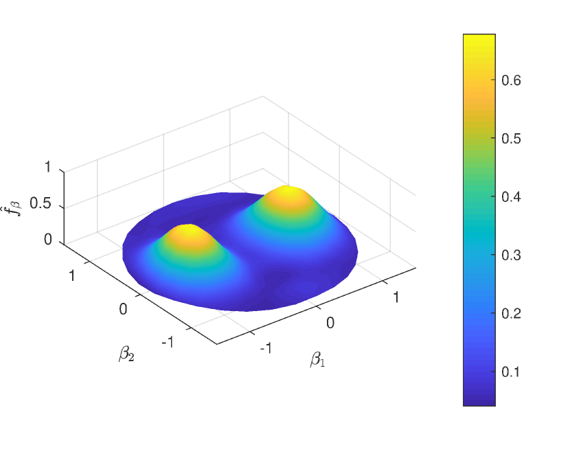
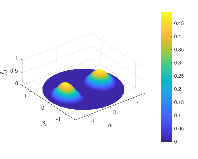
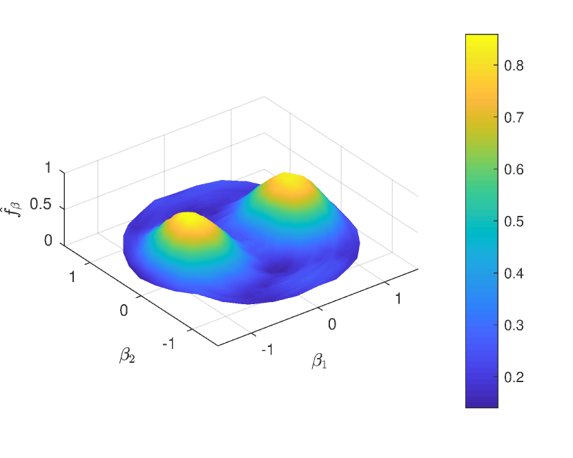
Figure 1 displays the distribution of estimates based on a Monte-Carlo experiments with 100 replications and $n=3000$. We plot the Lambert equal-area projection on the disk which is defined (see [22])

$$(\sin\theta\cos\phi,\sin\theta\sin\phi,\cos\theta)^{\top}\mapsto 2\sin\left(\frac{\theta}{2}\right)(\cos\phi,\sin\phi)^{\top}.$$

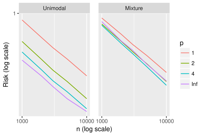
Our main contribution is a control of the estimation error for all ${\rm L}^{p}$ norm. Table 1 displays the expected risk, approximated using Monte-Carlo and 100 replications, for some ${\rm L}^{p}$ norms. More precisely, we have approximated the following renormalized quantities: $\left(\mathbb{E}\left[\left\|\widehat{f}_{\beta}-f_{\beta}\right\|_{p}^{p}\right]/\|f_{\beta}\|_{p}^{p}\right)^{1/p}$ for $p=\{1,2,4\}$ and $\mathbb{E}\left[\left\|\widehat{f}_{\beta}-f_{\beta}\right\|_{\infty}\right]/\|f_{\beta}\|_{\infty}$. Figure 2 displays the decay of those error with respect to $n$ in a logarithmic scales. As expected, we observe a simultaneous control over all norm and the error decays follows the power law given by the upper bounds. The results are similar to the one obtained in [10] except that our threshold does not depend on the unknown regularity of the function whereas the level used in [10] depends on it.

(a) True density

(b) Mean of estimates

(c) 5% quantile of estimates

(d) 95% quantile of estimates

(e) True density

(f) Mean of estimates

(g) 5% quantile of estimates

(h) 95% quantile of estimates

Figure 1: True density and distribution of the estimates.

	Unimodal					Mixture
	$1000$	$2000$	$3000$	$5000$	$10000$	$1000$	$2000$	$3000$	$5000$	$10000$
$\mathbb{E}\left[\left\|\widehat{f}_{\beta}-f_{\beta}\right\|_{1}\right]/\|f_{\beta}\|_{1}$	$0.89$	$0.64$	$0.53$	$0.43$	$0.32$	$0.92$	$0.68$	$0.57$	$0.46$	$0.34$
$\left(\mathbb{E}\left[\left\|\widehat{f}_{\beta}-f_{\beta}\right\|^{2}_{2}\right]/\|f_{\beta}\|_{2}^{2}\right)^{1/2}$	$0.6$	$0.43$	$0.35$	$0.29$	$0.21$	$0.82$1	$0.6$	$0.5$	$0.4$	$0.29$
$\left(\mathbb{E}\left[\left\|\widehat{f}_{\beta}-f_{\beta}\right\|^{4}_{4}\right]/\|f_{\beta}\|_{4}^{4}\right)^{1/4}$	$0.49$	$0.36$	$0.29$	$0.24$	$0.17$	$0.8$	$0.58$	$0.48$	$0.38$	$0.27$
$\mathbb{E}\left[\left\|\widehat{f}_{\beta}-f_{\beta}\right\|_{\infty}\right]/\|f_{\beta}\|_{\infty}$	$0.4$2	$0.32$	$0.26$	$0.21$	$0.17$	$0.86$	$0.6$	$0.51$	$0.39$	$0.29$

Table 1: Risk.

Figure 2: Decay of the risk with $n$ in logarithmic scales.

7 Appendix

7.1 A preliminary lemma

Lemma 10

The following equality holds for every $g\in{\rm L}^{2}({\mathbb{S}}^{d-1})$,

$$\langle R,g\rangle=2\mathbb{E}\left[\frac{Yg^{-}(X)}{f_{X}(X)}\right].$$

Proof. The result is based on the following

$$\langle R,g\rangle =\langle R,g^{-}\rangle\quad\mbox{(because $R$ is odd)}$$

$$=2\int_{H^{+}}\frac{R(x)g^{-}(x)}{f_{X}(x)}f_{X}(x)d\sigma(x)$$

$$=2\mathbb{E}\left[\frac{R(X)g^{-}(X)}{f_{X}(X)}\right]$$

$$=2\mathbb{E}\left[\frac{\mathbb{E}[Y|X]g^{-}(X)}{f_{X}(X)}\right].\qquad\qquad\qquad\qquad\qquad\square$$

7.2 Proof of Proposition 5

The operator $\mathcal{K}$ is related to the Hemispherical transform (see [10, 26]) defined for $f\in{\rm L}^{1}({\mathbb{S}}^{d-1})$ and a.e. $x\in{\mathbb{S}}^{d-1}$ by

$$\mathcal{H}(f)(x)\mathrel{\stackrel{{\scriptstyle\makebox[0.0pt]{\mbox{\tiny def}}}}{{=}}}\int_{{\mathbb{S}}^{d-1}}\mathbf{1}_{x^{\top}y>0}f(y)d\sigma(y),$$

through

$$Kf=2\mathcal{H}(f)-\int_{{\mathbb{S}}^{d-1}}f(y)d\sigma(y).$$

(P1.1) is a consequence of the fact that $y\to x^{\top}y\in{\rm L}^{\infty}_{{\rm odd}}({\mathbb{S}}^{d-1})$. (P1.2) follows from Theorem 2 (ii), and (P1.3) follows from Theorem C in [26]. The second part of the proposition together with (P1.4) are consequences of the properties of $\mathcal{H}$ detailed in [10]. The inequalities (9) correspond to Lemma A.2. Note however that there is a typo in the proof and we should read $1.3\ldots(2p-1)\asymp p^{-1/2}2.4\ldots(2p)$ but the result still holds.

7.3 Proof of Theorem 8

Start by noting that for every $j\in{\mathbb{N}}$ and $\xi\in\Xi_{j}$,

$$\int_{{\mathbb{S}}^{d-1}}\psi_{j,\xi}(x)dx=\omega(j,\xi)b(0)=\omega(j,\xi)(a(0)-a(0))=0.$$

This implies that the functions $f_{m}$ that we introduce below integrate to 1.

7.3.1 Proof of the lower bound in the dense zone

Consider the family $(P_{m})_{m=0}^{\mathcal{M}}$, where $\mathcal{M}\in{\mathbb{N}}^{*}$, of distributions of an i.i.d. sample of $(Y,X)$ of size $n$ when $f_{\beta}=f_{m}$ and the density of $X$ is $f_{X}$. These probabilities are absolutely continuous with respect to the product of $\delta_{1}+\delta_{-1}$, where $\delta_{y}$ denotes the Dirac mass at $y$ and $\sigma$. Take $j\in{\mathbb{N}}$, $f_{0}=1/\sigma({\mathbb{S}}^{d-1})$, and consider the set $A_{j}$ from Lemma 6 (ii). By the Varshamov-Guilbert bound (Lemma 2.9 in [27]) there exists $\Omega\subseteq\{0,1\}^{A_{j}}$ containing $(0,\ldots,0)$ such that $|\Omega|=2^{|A_{j}|/8}$ and $\forall(\omega_{1},\omega_{2})\in\Omega^{2}$, $\|\omega_{1}-\omega_{2}\|_{\ell^{1}}\geq|A_{j}|/8$. Enumerate the elements of $\Omega$ from 0 (corresponding to the zero vector) to $\mathcal{M}\mathrel{\stackrel{{\scriptstyle\makebox[0.0pt]{\mbox{\tiny def}}}}{{=}}}|\Omega|-1$ and define

$$f_{m}\mathrel{\stackrel{{\scriptstyle\makebox[0.0pt]{\mbox{\tiny def}}}}{{=}}}f_{0}+\gamma\sum_{\xi\in A_{j}}\omega_{\xi}\psi_{j,\xi}$$

when $(\omega_{\xi})_{\xi\in A_{j}}$ is the $m$th element of $\Omega$ and $\gamma=cC_{\Xi}^{-1/r}M2^{-j(s+(d-1)/2)}$ for $0<c<1$ such that all $f_{m}$ are nonnegative. We now use the following result (see Theorem 2.5 in [27]).

Lemma 11

If for $0<\alpha<1/8$ we have:

1. $f_{m}\in B_{r,q}^{s}(M)\cap\mathcal{D}$ for $m=0,\ldots,\mathcal{M}$,

2. $\forall\ 0\leq m<l\leq\mathcal{M},\ \|f_{m}-f_{l}\|_{p}\geq 2h>0$,

3. $\frac{1}{\mathcal{M}}\sum_{m=1}^{\mathcal{M}}K(P_{m},P_{0})\leq\alpha\ln(\mathcal{M})$,

then for every $z\geq 1$

$$\inf_{\widehat{f_{\beta}}}\sup_{f_{\beta}\in B^{s}_{r,q}(M)\cap\mathcal{D}}\mathbb{E}\left\|\widehat{f_{\beta}}-f_{\beta}\right\|_{p}^{z}\geq h^{z}\frac{\sqrt{\mathcal{M}}}{1+\sqrt{\mathcal{M}}}\left(1-2\alpha-\sqrt{\frac{2\alpha}{\ln(\mathcal{M})}}\right).$$ (29)

Start by checking (i) in Lemma 11. It is enough to show that $f_{m}\in B_{r,q}^{s}(M)$. Indeed, for $r\geq 1$ and $\omega\in\Omega$, we have $\left\|\left(\omega_{\xi}\right)_{\xi\in A_{j}}\right\|_{\ell^{r}}\leq\left\|\left(\omega_{\xi}\right)_{\xi\in A_{j}}\right\|_{\ell^{1}}^{1/r}\leq C_{\Xi}^{1/r}2^{j(d-1)/r}$, we obtain

$$\gamma 2^{j(s+(d-1)(1/2-1/r))}\left\|\left(\omega_{\xi}\right)_{\xi\in A_{j}}\right\|_{\ell^{r}}\leq\gamma C_{\Xi}^{1/r}2^{j(s+(d-1)/2)}\leq M.$$

Lemma 6 (ii) now yields that for every $1\leq p\leq\infty$ and $0\leq m<l\leq\mathcal{M}$

$$\left\|f_{m}-f_{l}\right\|_{p}\geq\gamma c_{p,A}2^{j(d-1)(1/2-1/p)}\left(\frac{c_{A}}{8}2^{j(d-1)}\right)^{1/p}=2h.$$

Thus (ii) in Lemma 11 follows with $h=c_{p,A}\left(\frac{c_{A}}{8}\right)^{1/p}cC_{\Xi}^{-1/r}M2^{-js-1}$.
By independence, the Kullback-Leibler divergence between $P_{m}$ and $P_{0}$ is given by

$$K(P_{m},P_{0})=n\mathbb{E}\left[\mathcal{H}(f_{m})(X)\ln\left(\frac{\mathcal{H}(f_{m})(X)}{\mathcal{H}(f_{0})(X)}\right)+\left(1-\mathcal{H}(f_{m})(X)\right)\ln\left(\frac{1-\mathcal{H}(f_{m})(X)}{1-\mathcal{H}(f_{0})(X)}\right)\right].$$

Using that, for $x>0$, $\ln(x)\leq x-1$, we obtain

$$K(P_{m},P_{0})\leq n\mathbb{E}\left[\frac{\mathcal{H}(f_{m}-f_{0})(X)^{2}}{\mathcal{H}(f_{0})(X)\left(1-\mathcal{H}(f_{0})(X)\right)}\right],$$

and thus

$$K(P_{m},P_{0}) \leq 4nA_{X}\left\|\mathcal{H}(f_{m}-f_{0})\right\|_{2}^{2}$$

$$\leq 4nA_{X}\lambda_{2^{j}+1,d}^{2}\left\|f_{m}-f_{0}\right\|_{2}^{2},$$

where the last display comes from the fact that $f_{m}-f_{0}\in\bigoplus_{2^{j}+1\leq k\leq 2^{j+2}-1}H^{k,d}$. From (9) we get

$$K(P_{m},P_{0})\leq 4C_{\lambda}(d)^{2}nA_{X}2^{-2j\nu(d)}\left\|f_{m}-f_{0}\right\|_{2}^{2},$$

which yields using Lemma 6 (i)

$$K(P_{m},P_{0}) \leq\left(2C_{\lambda}(d)C^{\prime}_{2}\gamma\right)^{2}nA_{X}2^{-2j\nu(d)}\left\|\left(\omega_{\xi}\right)_{\xi\in A_{j}}\right\|_{\ell^{2}}^{2}$$

$$\leq\left(2C_{\lambda}(d)C^{\prime}_{2}\gamma\right)^{2}nA_{X}2^{-2j\nu(d)}\left\|\left(\omega_{\xi}\right)_{\xi\in A_{j}}\right\|_{\ell^{1}}$$

$$\leq\left(2C_{\lambda}(d)C^{\prime}_{2}\gamma\right)^{2}C_{\Xi}nA_{X}2^{j(d-1-2\nu(d))}$$

$$\leq\left(2C_{\lambda}(d)C^{\prime}_{2}cM\right)^{2}C_{\Xi}^{1-2/r}nA_{X}2^{-2j(s+\nu(d))}.$$

Condition (iii) of Lemma 11 is satisfied once

$$\frac{2^{5}\left(C_{\lambda}(d)C^{\prime}_{2}cM\right)^{2}}{\ln(2)}C_{\Xi}^{-2/r}nA_{X}2^{-2j(s+\nu(d)+(d-1)/2)}\leq\alpha<\frac{1}{8}.$$ (30)

For $\alpha<1/8$, the lower bound (29) yields that

$$\inf_{\widehat{f_{\beta}}}\sup_{f_{\beta}\in B^{s}_{r,q}(M)}\mathbb{E}\left\|\widehat{f_{\beta}}-f_{\beta}\right\|_{p}^{z} \geq\left(c_{p,A}\left(\frac{c_{A}}{8}\right)^{1/p}cC_{\Xi}^{-1/r}M2^{-js-1}\right)^{z}\left(\frac{3}{4}-\frac{1}{2\sqrt{\ln(\mathcal{M})}}\right)$$

$$\geq\frac{1}{2}\left(c_{p,A}\left(\frac{c_{A}}{8}\right)^{1/p}cC_{\Xi}^{-1/r}\frac{M}{2}\right)^{z}2^{-jsz},$$

where the inequality leading to the second display holds when $\ln(\mathcal{M})\geq 4$, for example for $j(d-1)\geq\ln(5/c_{A}\ln(2))/\ln(2)$. Now (30) is satisfied for

$$j\geq j_{0}\mathrel{\stackrel{{\scriptstyle\makebox[0.0pt]{\mbox{\tiny def}}}}{{=}}}1+\frac{\ln\left(2^{8}\left(C_{\lambda}(d)C^{\prime}_{2}cM\right)^{2}C_{\Xi}^{-2/r}nA_{X}/\ln(2)\right)}{2\ln(2)(s+\nu(d)+(d-1)/2)},$$

which implies the lower bound

$$\inf_{\widehat{f_{\beta}}}\sup_{f_{\beta}\in B^{s}_{r,q}(M)}\mathbb{E}\left\|\widehat{f_{\beta}}-f_{\beta}\right\|_{p}^{z}$$

$$\geq\frac{1}{2}\left(c_{p,A}\left(\frac{c_{A}}{8}\right)^{1/p}cC_{\Xi}^{-1/r}M2^{-s-1}\right)^{z}\left(\frac{2^{8}\left(C_{\lambda}(d)C^{\prime}_{2}cM\right)^{2}C_{\Xi}^{-2/r}nA_{X}}{\ln(2)}\right)^{-\mu_{{\rm dense}}(d,p,r,s)z/2}.$$

7.3.2 Proof of the lower bound in the sparse zone

In this proof we consider asymptotic orders for simplicity. The various constants can be obtained like in Section 7.3.1. Consider the hypotheses

$$f_{m}=\frac{1}{\sigma({\mathbb{S}}^{d-1})}+\gamma\psi_{j,\xi_{m}},$$

where $\xi_{m}\in A_{j}$ and $|\gamma|\lesssim 2^{-j(d-1)/2}$ to ensure the functions are positive. The constant is adjusted so that for one of the $f_{m}$ that we denote $f_{0}$, $\forall x\in H^{+},\ \left|\mathcal{H}(f_{0}^{-})(x)\right|\leq c_{b}$ with $c_{b}\in(0,\frac{1}{2})$. The function $f_{m}$ also integrate to 1. We denote by $\mathcal{M}$ the cardinality of $A_{j}$ ($\mathcal{M}\simeq 2^{j(d-1)}$), $P_{m}$ the distributions of an i.i.d. sample of $(Y,X)$ of size $n$ when $f_{\beta}=f_{m}$ and for a given $f_{X}$, and $\Lambda(P_{m},P_{0})$ the likelihood ratio. Recall that $K(P_{m},P_{0})=\mathbb{E}_{P_{m}}\left[\Lambda(P_{m},P_{0})\right]$. We make use of the following Lemma from [20].

Lemma 12

If for $\pi_{0}>0$ and $\mathcal{M}\in{\mathbb{N}}^{*}$ the following three condition hold

1. $f_{m}\in B_{r,q}^{s}(M)\cap\mathcal{D}$ for $m=1,\ldots,\mathcal{M}$,

2. $\forall m\neq l,\ \|f_{m}-f_{l}\|_{p}\geq 2h>0$,

3. $\forall m=1,\ldots,\mathcal{M}$, $\Lambda(P_{0},P_{m})=\exp(z_{n}^{m}-v_{n}^{m})$, where $z_{n}^{m}$ are random variables and $v_{n}^{m}$ constants such that $\mathbb{P}(z_{n}^{m}>0)\geq\pi_{0}$ and $\exp\left(\sup_{m=1,\ldots,\mathcal{M}}v_{n}^{m}\right)\leq\mathcal{M}$,

then

$$\forall z\geq 1,\ \inf_{\widehat{f_{\beta}}}\sup_{f_{\beta}\in B^{s}_{r,q}(M)\cap\mathcal{D}}\mathbb{E}\left\|\widehat{f_{\beta}}-f_{\beta}\right\|_{p}^{z}\geq\frac{h^{-z}\pi_{0}}{2}.$$

Item (i) is satisfied when $|\gamma|\leq M2^{-j(s-(d-1)(1/r-1/2)}$. This is more restrictive than the condition to ensure positivity because we assume that $s\geq(d-1)/r$. Thus, now we take $\gamma=2cM2^{-j(s-(d-1)(1/r-1/2)}$ for a well-chosen constant $c$.
The constant $h$ in (ii) is obtained as follows, if $m\neq m^{\prime}$,

$$\|f_{m}-f_{m^{\prime}}\|_{p} =\gamma\|\psi_{j,\xi_{m}}-\psi_{j,\xi_{m^{\prime}}}\|_{p}$$

$$\geq\gamma c_{p,A}2^{j(d-1)(1/2-1/p)}$$

$$\geq 2cM2^{-j(s-(d-1)(1/r-1/p))}.$$

Let us now consider item (iii), we obtain

$$P_{m}\left(\log\left(\Lambda(P_{0},P_{m})\right)\geq-j(d-1)\log 2\right) \geq 1-P_{m}\left(\left|\log\left(\Lambda(P_{0},P_{m})\right)\right|\geq j(d-1)\log 2\right)$$

$$\geq 1-\frac{\mathbb{E}_{P_{m}}\left[\left|\log\left(\Lambda(P_{0},P_{m})\right)\right|\right]}{j(d-1)\log 2}.$$

Thus, condition (iii) is satisfied when

$$\mathbb{E}_{P_{m}}\left[\left|\log\left(\Lambda(P_{0},P_{m})\right)\right|\right]\leq\alpha j(d-1)\log 2,$$

for $\alpha\in(0,1)$. The same computations as in the beginning of Section 5.1 yield that we need to impose $n2^{-2j\nu(d)}\gamma^{2}\lesssim j$, thus

$$A_{X}n2^{-2j(s+\nu(d)-(d-1)(1/r-1/2))}\lesssim j.$$

The desired rate is obtained by taking

$$2^{j}\simeq\left(\frac{nA_{X}}{\log\left(nA_{X}\right)}\right)^{\frac{1}{2(s+\nu(d)-(d-1)(1/r-1/2))}}.$$

7.4 Comparison between Besov ellipsoids of a function and its odd part

Lemma 13

For $0<s,q\leq\infty$ and $1\leq r\leq\infty$, there exists a constant $c_{\mathrm{eq}}$ that can depend on $d$ such that, for every $f\in B^{s}_{r,q}$, $\|f^{-}\|_{B^{s}_{r,q}}\leq c_{\mathrm{eq}}\|f\|_{B^{s}_{r,q}}$.

Proof. In Definition 4 every $f\in B^{s}_{r,q}({\mathbb{S}}^{d-1})$ has same norm as $x\to f(-x)$, thus by the triangle inequality $\|f^{-}\|_{B^{s}_{r,q}}^{A}\leq\|f\|_{B^{s}_{r,q}}^{A}$. We conclude by equivalence of the norms. $\square$

7.5 A general inequality

We make use of the constants $c_{1,z}$ and $c_{2,z}$ such that

$$\int_{\mathbb{R}^{+}}z\tau^{z-1}e^{-\beta\tau}d\tau \leq c_{1,z}\beta^{-z}$$ (31)

$$\int_{\mathbb{R}^{+}}z\tau^{z-1}e^{-\alpha\tau^{2}}d\tau \leq c_{2,z}\alpha^{-z/2}.$$ (32)

Lemma 14

For every $\tau,\ \gamma,\ z>1$ and

$$T_{j,\xi,\gamma}^{s,++}\geq 3\sqrt{2\gamma}t_{n}\widehat{\sigma}_{j,\xi}+26M_{j,\xi}\frac{\gamma\log n}{n-1}\mathrel{\stackrel{{\scriptstyle\makebox[0.0pt]{\mbox{\tiny def}}}}{{=}}}T_{j,\xi,\gamma}^{s,+},$$

the two following inequalities hold:
when $p=\infty$,

$$\frac{1}{2^{z-1}}\mathbb{E}\left[\left\|\widehat{f_{\beta}}^{a,\rho}-f_{\beta}\right\|_{\infty}^{z}\right]$$

$$\leq\left\|{f_{\beta}^{-}}^{a,J}-{f_{\beta}^{-}}\right\|_{\infty}^{z}+(J+1)^{z-1}C^{\prime z}_{\infty}\Big{\{}$$

$$\qquad a_{n,\infty,z,J}\sum_{j=0}^{J}2^{j(d-1)z/2}\left(\sup_{\xi\in\Xi_{j}}\left|\beta^{a}_{j,\xi}\right|^{z}\mathbf{1}_{\left|\beta^{a}_{j,\xi}\right|\leq T^{s,++}_{j,\xi,\gamma}}+\mathbb{E}\left[\sup_{\xi\in\Xi_{j}}\left|\widehat{\beta}^{a}_{j,\xi}-\beta^{a}_{j,\xi}\right|^{z}\mathbf{1}_{\left|\beta^{a}_{j,\xi}\right|>T^{s,++}_{j,\xi,\gamma}}\right]\right)$$

$$\qquad+\frac{4C_{\Xi}}{n^{\gamma}}\sum_{j=0}^{J}2^{j(d-1)(z/2+1)}\sup_{\xi\in\Xi_{j}}\left|\beta^{a}_{j,\xi}\right|^{z}$$

$$\qquad+\left(\frac{C_{\Xi}4}{n^{\gamma}}\right)^{1-1/\tau}\left(\frac{1}{\sqrt{n}}B_{X}^{1/2}2^{Jz(\nu(d)+(d-1)/2)}\right)^{z}2^{J(d-1)(1-1/\tau)}b_{n,\infty,z,J,\tau}\Big{\}},$$

where

$$a_{n,\infty,z,J} =1+\left(\frac{2}{\sqrt{\gamma\log n}}\right)^{z}\left(2+\left(\log\left(C_{\Xi}2^{J(d-1)}c_{2,z}\right)\right)^{z/2}\right)$$

$$\quad+\left(\frac{4}{\gamma\log n}\right)^{z}\left(2+\left(\log\left(C_{\Xi}2^{J(d-1)}c_{1,z}\right)\right)^{z}\right)$$

$$b_{n,\infty,z,J,\tau} =\frac{\left(2\sqrt{2}C_{2}B(d,2)\right)^{z}\left(2^{1/\tau}+\left(\log\left(C_{\Xi}2^{J(d-1)}c_{2,z\tau}\right)\right)^{z/2}\right)}{1-2^{-(z\nu(d)+(d-1)(z/2+1-1/\tau))}}$$

$$\quad+\frac{\left(8C_{\infty}B(d,\infty)/3\right)^{z}\left(2^{1/\tau}+\left(\log\left(C_{\Xi}2^{J(d-1)}c_{1,z}\right)\right)^{z}\right)}{1-2^{-(z\nu(d)+(d-1)(z+1-1/\tau))}}\left(\frac{2^{J(d-1)}}{n}B_{X}\right)^{z/2};$$

while, when $1\leq p\leq\infty$,

$$\frac{1}{2^{z-1}}\mathbb{E}\left[\left\|\widehat{f_{\beta}}^{a,\rho}-f_{\beta}\right\|_{p}^{z}\right]$$

$$\leq\left\|{f_{\beta}^{-}}^{a,J}-{f_{\beta}^{-}}\right\|_{p}^{z}+(J+1)^{z-1}C^{\prime z}_{p}C_{\Xi}^{z/(p\wedge z)-1}\Big{\{}$$

$$\qquad a_{n,p,z,J}\sum_{j=0}^{J}2^{j(d-1)(z/2-z/(p\vee z))}\sum_{\xi\in\Xi_{j}}\left(\left|\beta^{a}_{j,\xi}\right|^{z}\mathbf{1}_{\left|\beta^{a}_{j,\xi}\right|\leq T^{s,++}_{j,\xi,\gamma}}+\mathbb{E}\left[\left|\widehat{\beta}^{a}_{j,\xi}-\beta^{a}_{j,\xi}\right|^{z}\right]\mathbf{1}_{\left|\beta^{a}_{j,\xi}\right|>T^{s,++}_{j,\xi,\gamma}}\right)$$

$$\qquad+\frac{4}{n^{\gamma}}\sum_{j=0}^{J}2^{j(d-1)z(1/2-1/(p\vee z))}\sum_{\xi\in\Xi_{j}}\left|\beta^{a}_{j,\xi}\right|^{z}$$

$$\qquad+\frac{2^{2-1/\tau}}{n^{\gamma(1-\frac{1}{\tau})}}C_{\Xi}\left(\frac{1}{\sqrt{n}}B_{X}^{1/2}2^{J(\nu(d)+(d-1)/2)}\right)^{z}2^{J(d-1)(1-z/(p\vee z))}b_{n,p,z,J,\tau}\Big{\}},$$

where

$$a_{n,p,z,J} =1+2\left(\left(\frac{\sqrt{2}c_{2,z}^{1/z}}{\sqrt{\gamma\log n}}\right)^{z}+\left(\frac{2c_{1,z}^{1/z}}{\gamma\log n}\right)^{z}\right)$$

$$b_{n,p,z,J,\tau} =\frac{\left(2c_{2,z\tau}^{1/(z\tau)}C_{2}B(d,2)\right)^{z}}{1-2^{-(z\nu(d)+(d-1)(z/2+1-z/(p\vee z)))}}+\frac{\left(\frac{4}{3}c_{1,z\tau}^{1/(z\tau)}C_{\infty}B(d,\infty)\right)^{z}}{1-2^{-(z\nu(d)+(d-1)(z+1-z/(p\vee z)))}}\left(\frac{2^{J(d-1)}}{n}B_{X}\right)^{z/2}.$$

The inequalities of Lemma 14 are similar to oracle inequalities, for a well-chosen $J$ depending on $n$ (see Theorem 9), where the oracle estimates $\beta^{a}_{j,\xi}$ if and only if the error made by estimating this coefficient is smaller than the one made by discarding it. This oracle strategy would lead to a quantity of the form

$$\left|\beta^{a}_{j,\xi}\right|^{z}\mathbf{1}_{\left|\beta^{a}_{j,\xi}\right|\leq\left(\mathbb{E}\left[\left|\widehat{\beta}^{a}_{j,\xi}-\beta^{a}_{j,\xi}\right|^{z}\right]\right)^{1/z}}+\mathbb{E}\left[\left|\widehat{\beta}^{a}_{j,\xi}-\beta^{a}_{j,\xi}\right|^{z}\right]\mathbf{1}_{\left|\beta^{a}_{j,\xi}\right|>\left(\mathbb{E}\left[\left|\widehat{\beta}^{a}_{j,\xi}-\beta^{a}_{j,\xi}\right|^{z}\right]\right)^{1/z}}.$$

Proving such an oracle inequality would require to lower bound $\left(\mathbb{E}\left[\left|\widehat{\beta}^{a}_{j,\xi}-\beta^{a}_{j,\xi}\right|^{z}\right]\right)^{1/z}$. In the inequalities of Lemma 14 the ideal quantity $\left(\mathbb{E}\left[\left|\widehat{\beta}^{a}_{j,\xi}-\beta^{a}_{j,\xi}\right|^{z}\right]\right)^{1/z}$ is replaced by $T_{j,\xi,\gamma}^{s,++}$, called quasi-oracle. The remaining terms can be made as small as we want by taking $\gamma$ large enough. The last term corresponds to the approximation error. Upper bounds of these types, uniform on Besov ellipsoids, yield an approximation error which can be expressed in terms of the regularity of the Besov class and is uniformly small for $J$ large enough and allows to treat the bias/variance trade-off in the quasi-oracle term uniformly over the ellipsoid.

7.6 Proof of Lemma 14

7.6.1 Preliminaries

Recall from the proof of Theorem 4.1 in [10] that for every $1\leq p\leq\infty$

$$\left\|\widehat{f_{\beta}}^{a,\rho}-f_{\beta}\right\|_{p}\leq 2\left\|\widehat{{f_{\beta}^{-}}}^{a,\rho}-{f_{\beta}^{-}}\right\|_{p},$$

and that, for $1\leq z<\infty$, we have

$$\left\|\widehat{{f_{\beta}^{-}}}^{a,\rho}-{f_{\beta}^{-}}\right\|_{p}^{z}\leq 2^{z-1}\left(\left\|\widehat{{f_{\beta}^{-}}}^{a,\rho}-{f_{\beta}^{-}}^{a,J}\right\|_{p}^{z}+\left\|{f_{\beta}^{-}}^{a,J}-{f_{\beta}^{-}}\right\|_{p}^{z}\right).$$ (33)

The first term corresponds to the error in the high dimensional space while the second term corresponds to the approximation error. Let us start by studying the first term.
Lemma 6 (i) yields

$$\left\|\widehat{{f_{\beta}^{-}}}^{a,\rho}-{f_{\beta}^{-}}^{a,J}\right\|_{p}^{z} \leq(J+1)^{z-1}\sum_{j=0}^{J}\left\|\sum_{\xi\in\Xi_{j}}\left(\rho_{T_{j,\xi,\gamma}}\left(\widehat{\beta}^{a}_{j,\xi}\right)-\beta^{a}_{j,\xi}\right)\psi_{j,\xi}\right\|_{p}^{z}$$

$$\leq(J+1)^{z-1}\sum_{j=0}^{J}C^{\prime z}_{p}2^{j(d-1)z(1/2-1/p)}\left\|\rho_{T_{j,\xi,\gamma}}\left(\widehat{\beta}^{a}_{j,\xi}\right)-\beta^{a}_{j,\xi}\right\|_{p}^{z}.$$

Thus, for $p=\infty$, we have

$$\left\|\widehat{{f_{\beta}^{-}}}^{a,\rho}-{f_{\beta}^{-}}^{a,J}\right\|_{p}^{z} \leq(J+1)^{z-1}\sum_{j=0}^{J}C^{\prime z}_{\infty}2^{j(d-1)z/2}\sup_{\xi\in\Xi_{j}}\left|\rho_{T_{j,\xi,\gamma}}\left(\widehat{\beta}^{a}_{j,\xi}\right)-\beta^{a}_{j,\xi}\right|^{z},$$

while, for $p<\infty$, we have

$$\left\|\widehat{{f_{\beta}^{-}}}^{a,\rho}-{f_{\beta}^{-}}^{a,J}\right\|_{p}^{z} \leq(J+1)^{z-1}C^{\prime z}_{p}C_{\Xi}^{z/(p\wedge z)-1}\sum_{j=0}^{J}2^{j(d-1)z(1/2-1/(p\vee z))}\sum_{\xi\in\Xi_{j}}\left|\rho_{T_{j,\xi,\gamma}}\left(\widehat{\beta}^{a}_{j,\xi}\right)-\beta^{a}_{j,\xi}\right|^{z}.$$

The last inequality is obtained by using that, when $p\geq z$, we have

$$\left(\sum_{\xi\in\Xi_{j}}\left|b_{\xi}\right|^{p}\right)^{z/p}\leq\sum_{\xi\in\Xi_{j}}\left|b_{\xi}\right|^{z},$$

and by the Hölder inequality, when $p\leq z$, we have

$$\left(\sum_{\xi\in\Xi_{j}}\left|b_{\xi}\right|^{p}\right)^{z/p}\leq C_{\Xi}^{z/p-1}\sum_{\xi\in\Xi_{j}}\left|b_{\xi}\right|^{z}.$$

7.6.2 Coefficientwise analysis

For the simplicity of the notations we sometimes drop the dependence on $\gamma$ in the sets of indices.
We first consider the term

$$\delta_{j,\xi,z} \mathrel{\stackrel{{\scriptstyle\makebox[0.0pt]{\mbox{\tiny def}}}}{{=}}}\left|\rho_{T_{j,\xi,\gamma}}\left(\widehat{\beta}^{a}_{j,\xi}\right)-\beta^{a}_{j,\xi}\right|^{z}.$$

By construction we have

$$\delta_{j,\xi,z} =\left|\beta^{a}_{j,\xi}\right|^{z}\mathbf{1}_{\left|\widehat{\beta}^{a}_{j,\xi}\right|\leq T_{j,\xi,\gamma}}+\left|\widehat{\beta}^{a}_{j,\xi}-\beta^{a}_{j,\xi}\right|^{z}\mathbf{1}_{\left|\widehat{\beta}^{a}_{j,\xi}\right|>T_{j,\xi,\gamma}}$$

$$=\max\left(\left|\beta^{a}_{j,\xi}\right|^{z}\mathbf{1}_{\left|\widehat{\beta}^{a}_{j,\xi}\right|\leq T_{j,\xi,\gamma}},\left|\widehat{\beta}^{a}_{j,\xi}-\beta^{a}_{j,\xi}\right|^{z}\mathbf{1}_{\left|\widehat{\beta}^{a}_{j,\xi}\right|>T_{j,\xi,\gamma}}\right).$$

We introduce two “phantom” random thresholds $T^{b}_{j,\xi,\gamma}=T_{j,\xi,\gamma}-\Delta_{j,\xi,\gamma}$ and $T^{s}_{j,\xi,\gamma}=T_{j,\xi,\gamma}+\Delta_{j,\xi,\gamma}$ for some $\Delta_{j,\xi,\gamma}$ to be defined later. They are used to define big and small original needlet coefficients. We also use $T^{b,-}_{j,\xi,\gamma}$ for a deterministic lower bound on $T^{b}_{j,\xi,\gamma}$, $T^{s,+}_{j,\xi,\gamma}$ and $\Delta^{+}_{j,\xi,\gamma}$ for deterministic upper bounds on $T^{s}_{j,\xi,\gamma}$ and $\Delta_{j,\xi,\gamma}$. These bounds will hold with high probability. We obtain almost surely

$$\delta_{j,\xi,z} =\max\bigg{(}\left|\beta^{a}_{j,\xi}\right|^{z}\max\left(\mathbf{1}_{\left|\widehat{\beta}^{a}_{j,\xi}\right|\leq T_{j,\xi,\gamma}}\mathbf{1}_{\left|\beta^{a}_{j,\xi}\right|\leq T^{s}_{j,\xi,\gamma}},\mathbf{1}_{\left|\widehat{\beta}^{a}_{j,\xi}\right|\leq T_{j,\xi,\gamma}}\mathbf{1}_{\left|\beta^{a}_{j,\xi}\right|>T^{s}_{j,\xi,\gamma}}\right),$$

$$\qquad\qquad\left|\widehat{\beta}^{a}_{j,\xi}-\beta^{a}_{j,\xi}\right|^{z}\max\left(\mathbf{1}_{\left|\widehat{\beta}^{a}_{j,\xi}\right|>T_{j,\xi,\gamma}}\mathbf{1}_{\left|\beta^{a}_{j,\xi}\right|\leq T^{b}_{j,\xi,\gamma}},\mathbf{1}_{\left|\widehat{\beta}^{a}_{j,\xi}\right|>T_{j,\xi,\gamma}}\mathbf{1}_{\left|\beta^{a}_{j,\xi}\right|>T^{b}_{j,\xi,\gamma}}\right)\bigg{)}$$

$$\leq\max\bigg{(}\left|\beta^{a}_{j,\xi}\right|^{z}\max\left(\mathbf{1}_{\left|\beta^{a}_{j,\xi}\right|\leq T^{s}_{j,\xi,\gamma}},\mathbf{1}_{\left|\widehat{\beta}^{a}_{j,\xi}-\beta^{a}_{j,\xi}\right|>\Delta_{j,\xi,\gamma}}\right),$$

$$\qquad\qquad\left|\widehat{\beta}^{a}_{j,\xi}-\beta^{a}_{j,\xi}\right|^{z}\max\left(\mathbf{1}_{\left|\widehat{\beta}^{a}_{j,\xi}-\beta^{a}_{j,\xi}\right|>\Delta_{j,\xi,\gamma}},\mathbf{1}_{\left|\beta^{a}_{j,\xi}\right|>T^{b}_{j,\xi,\gamma}}\right)\bigg{)}$$

$$\leq\max\bigg{(}\left|\beta^{a}_{j,\xi}\right|^{z}\max\left(\mathbf{1}_{\left|\beta^{a}_{j,\xi}\right|\leq T^{s,+}_{j,\xi,\gamma}},\mathbf{1}_{T^{s,+}_{j,\xi,\gamma}<T^{s}_{j,\xi,\gamma}},\mathbf{1}_{\left|\widehat{\beta}^{a}_{j,\xi}-\beta^{a}_{j,\xi}\right|>\Delta_{j,\xi,\gamma}}\right),$$

$$\qquad\qquad\left|\widehat{\beta}^{a}_{j,\xi}-\beta^{a}_{j,\xi}\right|^{z}\max\left(\mathbf{1}_{\left|\widehat{\beta}^{a}_{j,\xi}-\beta^{a}_{j,\xi}\right|>\Delta_{j,\xi,\gamma}},\mathbf{1}_{\left|\beta^{a}_{j,\xi}\right|>T^{b,-}_{j,\xi,\gamma}},\mathbf{1}_{T^{b,-}_{j,\xi,\gamma}>T^{b}_{j,\xi,\gamma}}\right)\bigg{)}.$$

Sorting the terms according to the number of random terms we obtain

$$\delta_{j,\xi,z} \leq\max\bigg{(}\left|\beta^{a}_{j,\xi}\right|^{z}\mathbf{1}_{\left|\beta^{a}_{j,\xi}\right|\leq T^{s,+}_{j,\xi,\gamma}},\left|\beta^{a}_{j,\xi}\right|^{z}\max\left(\mathbf{1}_{T^{s,+}_{j,\xi,\gamma}<T^{s}_{j,\xi,\gamma}},\mathbf{1}_{\left|\widehat{\beta}^{a}_{j,\xi}-\beta^{a}_{j,\xi}\right|>\Delta_{j,\xi,\gamma}}\right),$$

$$\qquad\qquad\left|\widehat{\beta}^{a}_{j,\xi}-\beta^{a}_{j,\xi}\right|^{z}\mathbf{1}_{\left|\beta^{a}_{j,\xi}\right|>T^{b,-}_{j,\xi,\gamma}},\left|\widehat{\beta}^{a}_{j,\xi}-\beta^{a}_{j,\xi}\right|^{z}\max\left(\mathbf{1}_{\left|\widehat{\beta}^{a}_{j,\xi}-\beta^{a}_{j,\xi}\right|>\Delta_{j,\xi,\gamma}},\mathbf{1}_{T^{b,-}_{j,\xi,\gamma}>T^{b}_{j,\xi,\gamma}}\right)\bigg{)}.$$

7.6.3 Scalewise analysis

Defining

$$M_{j,z} \mathrel{\stackrel{{\scriptstyle\makebox[0.0pt]{\mbox{\tiny def}}}}{{=}}}\sup_{\xi\in\Xi_{j}}\left|\rho_{T_{j,\xi,\gamma}}\left(\widehat{\beta}^{a}_{j,\xi}\right)-\beta^{a}_{j,\xi}\right|^{z}=\sup_{\xi\in\Xi_{j}}\delta_{j,\xi,z}$$

$$S_{j,z} \mathrel{\stackrel{{\scriptstyle\makebox[0.0pt]{\mbox{\tiny def}}}}{{=}}}\sum_{\xi\in\Xi_{j}}\left|\rho_{T_{j,\xi,\gamma}}\left(\widehat{\beta}^{a}_{j,\xi}\right)-\beta^{a}_{j,\xi}\right|^{z}=\sum_{\xi\in\Xi_{j}}\delta_{j,\xi,z},$$

we obtain

$$M_{j,z} \leq\max\bigg{(}\sup_{\xi\in\Xi_{j}}\left|\beta^{a}_{j,\xi}\right|^{z}\mathbf{1}_{\left|\beta^{a}_{j,\xi}\right|\leq T^{s,+}_{j,\xi,\gamma}},\sup_{\xi\in\Xi_{j}}\left|\beta^{a}_{j,\xi}\right|^{z}\max\left(\mathbf{1}_{T^{s,+}_{j,\xi,\gamma}<T^{s}_{j,\xi,\gamma}},\mathbf{1}_{\left|\widehat{\beta}^{a}_{j,\xi}-\beta^{a}_{j,\xi}\right|>\Delta_{j,\xi,\gamma}}\right),$$

$$\quad\sup_{\xi\in\Xi_{j}}\left|\widehat{\beta}^{a}_{j,\xi}-\beta^{a}_{j,\xi}\right|^{z}\mathbf{1}_{\left|\beta^{a}_{j,\xi}\right|>T^{b,-}_{j,\xi,\gamma}},\sup_{\xi\in\Xi_{j}}\left|\widehat{\beta}^{a}_{j,\xi}-\beta^{a}_{j,\xi}\right|^{z}\max\left(\mathbf{1}_{T^{b,-}_{j,\xi,\gamma}>T^{b}_{j,\xi,\gamma}},\mathbf{1}_{\left|\widehat{\beta}^{a}_{j,\xi}-\beta^{a}_{j,\xi}\right|>\Delta_{j,\xi,\gamma}}\right)\bigg{)}$$

$$\mathrel{\stackrel{{\scriptstyle\makebox[0.0pt]{\mbox{\tiny def}}}}{{=}}}\max(M_{j,z}^{S0},M_{j,z}^{S1},M_{j,z}^{B1},M_{j,z}^{B2})$$

$$\leq M_{j,z}^{S0}+M_{j,z}^{S1}+M_{j,z}^{B1}+M_{j,z}^{B2};$$

$$S_{j,z} \leq\sum_{\xi\in\Xi_{j}}\left|\beta^{a}_{j,\xi}\right|^{z}\mathbf{1}_{\left|\beta^{a}_{j,\xi}\right|\leq T^{s,+}_{j,\xi,\gamma}}+\sum_{\xi\in\Xi_{j}}\left|\beta^{a}_{j,\xi}\right|^{z}\max\left(\mathbf{1}_{T^{s,+}_{j,\xi,\gamma}<T^{s}_{j,\xi,\gamma}},\mathbf{1}_{\left|\widehat{\beta}^{a}_{j,\xi}-\beta^{a}_{j,\xi}\right|>\Delta_{j,\xi,\gamma}}\right)$$

$$\quad+\sum_{\xi\in\Xi_{j}}\left|\widehat{\beta}^{a}_{j,\xi}-\beta^{a}_{j,\xi}\right|^{z}\mathbf{1}_{\left|\beta^{a}_{j,\xi}\right|>T^{b,-}_{j,\xi,\gamma}}+\sum_{\xi\in\Xi_{j}}\left|\widehat{\beta}^{a}_{j,\xi}-\beta^{a}_{j,\xi}\right|^{z}\max\left(\mathbf{1}_{T^{b,-}_{j,\xi,\gamma}>T^{b}_{j,\xi,\gamma}},\mathbf{1}_{\left|\widehat{\beta}^{a}_{j,\xi}-\beta^{a}_{j,\xi}\right|>\Delta_{j,\xi,\gamma}}\right)$$

$$\mathrel{\stackrel{{\scriptstyle\makebox[0.0pt]{\mbox{\tiny def}}}}{{=}}}S_{j,z}^{S0}+S_{j,z}^{S1}+S_{j,z}^{B1}+S_{j,z}^{B2}.$$

We bound the expectations of the random terms as follows

$$\mathbb{E}\left[M_{j,z}^{S1}\right] \leq\sup_{\xi\in\Xi_{j}}\left|\beta^{a}_{j,\xi}\right|^{z}\mathbb{E}\left[\sup_{\xi\in\Xi_{j}}\max\left(\mathbf{1}_{T^{s,+}_{j,\xi,\gamma}<T^{s}_{j,\xi,\gamma}},\mathbf{1}_{\left|\widehat{\beta}^{a}_{j,\xi}-\beta^{a}_{j,\xi}\right|>\Delta_{j,\xi,\gamma}}\right)\right]$$

$$\leq\sup_{\xi\in\Xi_{j}}\left|\beta^{a}_{j,\xi}\right|^{z}\left(\mathbb{P}\left(\bigcup_{\xi\in\Xi_{j}}\left\{T^{s,+}_{j,\xi,\gamma}<T^{s}_{j,\xi,\gamma}\right\}\right)+\mathbb{P}\left(\bigcup_{\xi\in\Xi_{j}}\left\{\left|\widehat{\beta}^{a}_{j,\xi}-\beta^{a}_{j,\xi}\right|>\Delta_{j,\xi,\gamma}\right\}\right)\right);$$

$$\mathbb{E}\left[M_{j,z}^{B1}\right] \leq\mathbb{E}\left[\sup_{\xi\in\Xi_{j}}\left|\widehat{\beta}^{a}_{j,\xi}-\beta^{a}_{j,\xi}\right|^{z}\mathbf{1}_{\left|\beta^{a}_{j,\xi}\right|>T^{b,-}_{j,\xi,\gamma}}\right];$$

$$\mathbb{E}\left[M_{j,z}^{B2}\right] \leq\mathbb{E}\left[\sup_{\xi\in\Xi_{j}}\left|\widehat{\beta}^{a}_{j,\xi}-\beta^{a}_{j,\xi}\right|^{z\tau}\right]^{1/\tau}\mathbb{E}\left[\sup_{\xi\in\Xi_{j}}\max\left(\mathbf{1}_{T^{b,-}_{j,\xi,\gamma}>T^{b}_{j,\xi,\gamma}},\mathbf{1}_{\left|\widehat{\beta}^{a}_{j,\xi}-\beta^{a}_{j,\xi}\right|>\Delta_{j,\xi,\gamma}}\right)\right]^{1-1/\tau}$$

$$\leq\mathbb{E}\left[\sup_{\xi\in\Xi_{j}}\left|\widehat{\beta}^{a}_{j,\xi}-\beta^{a}_{j,\xi}\right|^{z\tau}\right]^{1/\tau}\left(\mathbb{P}\left(\bigcup_{\xi\in\Xi_{j}}\left\{T^{b,-}_{j,\xi,\gamma}>T^{b}_{j,\xi,\gamma}\right\}\right)+\mathbb{P}\left(\bigcup_{\xi\in\Xi_{j}}\left\{\left|\widehat{\beta}^{a}_{j,\xi}-\beta^{a}_{j,\xi}\right|>\Delta_{j,\xi,\gamma}\right\}\right)\right)^{1-1/\tau};$$

$$\mathbb{E}\left[S_{j,z}^{S1}\right] =\sum_{\xi\in\Xi_{j}}\left|\beta^{a}_{j,\xi}\right|^{z}\mathbb{E}\left[\max\left(\mathbf{1}_{T^{s,+}_{j,\xi,\gamma}<T^{s}_{j,\xi,\gamma}},\mathbf{1}_{\left|\widehat{\beta}^{a}_{j,\xi}-\beta^{a}_{j,\xi}\right|>\Delta_{j,\xi,\gamma}}\right)\right]$$

$$\leq\sum_{\xi\in\Xi_{j}}\left|\beta^{a}_{j,\xi}\right|^{z}\left(\mathbb{P}\left\{T^{s,+}_{j,\xi,\gamma}<T^{s}_{j,\xi,\gamma}\right\}+\mathbb{P}\left\{\left|\widehat{\beta}^{a}_{j,\xi}-\beta^{a}_{j,\xi}\right|>\Delta_{j,\xi,\gamma}\right\}\right);$$

$$\mathbb{E}\left[S_{j,z}^{B1}\right] =\sum_{\xi\in\Xi_{j}}\mathbb{E}\left[\left|\widehat{\beta}^{a}_{j,\xi}-\beta^{a}_{j,\xi}\right|^{z}\right]\mathbf{1}_{\left|\beta^{a}_{j,\xi}\right|>T^{b,-}_{j,\xi,\gamma}};$$

$$\mathbb{E}\left[S_{j,z}^{B2}\right] =\sum_{\xi\in\Xi_{j}}\mathbb{E}\left[\left|\widehat{\beta}^{a}_{j,\xi}-\beta^{a}_{j,\xi}\right|^{z}\max\left(\mathbf{1}_{T^{b,-}_{j,\xi,\gamma}>T^{b}_{j,\xi,\gamma}},\mathbf{1}_{\left|\widehat{\beta}^{a}_{j,\xi}-\beta^{a}_{j,\xi}\right|>\Delta_{j,\xi,\gamma}}\right)\right]$$

$$\leq\sum_{\xi\in\Xi_{j}}\left(\mathbb{E}\left[\left|\widehat{\beta}^{a}_{j,\xi}-\beta^{a}_{j,\xi}\right|^{z\tau}\right]\right)^{1/\tau}\left(\mathbb{P}\left\{T^{b,-}_{j,\xi,\gamma}>T^{b}_{j,\xi,\gamma}\right\}+\mathbb{P}\left\{\left|\widehat{\beta}^{a}_{j,\xi}-\beta^{a}_{j,\xi}\right|>\Delta_{j,\xi,\gamma}\right\}\right)^{1-1/\tau}.$$

The constant $\tau>1$ in the Hölder inequality will be specified later.

7.6.4 Bernstein inequality and the term $\left|\widehat{\beta}^{a}_{j,\xi}-\beta^{a}_{j,\xi}\right|^{z}$

Let denote variance of $G_{j,\xi}(X,Y)$

$$\sigma_{j,\xi}^{2}\mathrel{\stackrel{{\scriptstyle\makebox[0.0pt]{\mbox{\tiny def}}}}{{=}}}\mathbb{E}\left[\left(G_{j,\xi}(X,Y)-\beta^{a}_{j,\xi}\right)^{2}\right].$$

Lemma 15

We have

$$\mathbb{E}\left[\left|\widehat{\beta}^{a}_{j,\xi}-\beta^{a}_{j,\xi}\right|^{z}\right]\leq 2\left(c_{2,z}\left(\frac{2}{\sqrt{n}}\sigma_{j,\xi}\right)^{z}+c_{1,z}\left(\frac{4}{3n}M_{j,\xi}\right)^{z}\right).$$

Proof. The Bernstein inequality yields

$$\mathbb{P}\left\{\left|\widehat{\beta}^{a}_{j,\xi}-\beta^{a}_{j,\xi}\right|\geq u\right\} \leq 2e^{-\frac{nu^{2}}{2\left(\left(\sigma_{j,\xi}\right)^{2}+M_{j,\xi}u/3\right)}}$$

$$\leq 2\left(e^{-\frac{nu^{2}}{4\left(\sigma_{j,\xi}\right)^{2}}}+e^{-\frac{3nu}{4M_{j,\xi}}}\right).$$

Using now $\mathbb{E}\left[|X|^{z}\right]=\int_{\mathbb{R}^{+}}zu^{z-1}\mathbb{P}\{|X|>u\}du$, we obtain

$$\mathbb{E}\left[\left|\widehat{\beta}^{a}_{j,\xi}-\beta^{a}_{j,\xi}\right|^{z}\right] \leq\int_{\mathbb{R}^{+}}zu^{z-1}\mathbb{P}\left\{\left|\widehat{\beta}^{a}_{j,\xi}-\beta^{a}_{j,\xi}\right|\geq u\right\}du$$

$$\leq\int_{\mathbb{R}^{+}}zu^{z-1}2\left(e^{-\frac{nu^{2}}{4\left(\sigma_{j,\xi}\right)^{2}}}+e^{-\frac{3nu}{4M_{j,\xi}}}\right)du,$$

hence the inequality from the lemma follows from (31) and (32). $\square$

Lemma 15 is used to obtain a uniform upper bound of the power of the ratio between $\left|\widehat{\beta}^{a}_{j,\xi}-\beta^{a}_{j,\xi}\right|$ and a threshold $c_{\sigma}\sqrt{\log(n)/n}\sigma_{j,\xi}+c_{M}\log(n)/(n-1)M_{j,\xi}$:

$$\mathbb{E}\left[\left(\frac{\left|\widehat{\beta}^{a}_{j,\xi}-\beta^{a}_{j,\xi}\right|}{c_{\sigma}\sqrt{\log(n)/n}\sigma_{j,\xi}+c_{M}\log(n)/(n-1)M_{j,\xi}}\right)^{z}\right] \leq 2\left(c_{2,z}\left(2\frac{1}{c_{\sigma}\sqrt{\log n}+c_{M}\frac{\sqrt{n}\log n}{n-1}\frac{M_{j,\xi}}{\sigma_{j,\xi}}}\right)^{z}\right.$$

$$\quad\left.+c_{1,z}\left(\frac{4}{3}\frac{1}{c_{\sigma}\sqrt{n}\sqrt{\log n}\frac{\sigma_{j,\xi}}{M_{j,\xi}}+c_{M}\log(n)\frac{n}{n-1}}\right)^{z}\right)$$

$$\leq 2\left(c_{2,z}\left(2\frac{1}{c_{\sigma}\sqrt{\log n}}\right)^{z}+c_{1,z}\left(\frac{4}{3}\frac{1}{c_{M}\log n}\right)^{z}\right).$$ (34)

The following similar lemma is useful to handle the case $p=\infty$.

Lemma 16

For any $\Xi^{\prime}_{j}\subset\Xi_{j}$, we have

$$\mathbb{E}\left[\sup_{\xi\in\Xi^{\prime}_{j}}\left(\frac{\left|\widehat{\beta}^{a}_{j,\xi}-\beta^{a}_{j,\xi}\right|}{u_{j,\xi}}\right)^{z}\right] \leq\left(\frac{2\sqrt{2}}{\sqrt{n}}\sup_{\xi\in\Xi^{\prime}_{j}}\frac{\sigma_{j,\xi}}{c_{j,\xi}}\right)^{z}\left(2+\left(\log\left(c_{2,z}\left|\Xi^{\prime}_{j}\right|\right)\right)^{z/2}\right)$$

$$\quad+\left(\frac{8}{3n}\sup_{\xi\in\Xi^{\prime}_{j}}\frac{M_{j,\xi}}{c_{j,\xi}}\right)^{z}\left(2+\left(\log\left(c_{1,z}\left|\Xi^{\prime}_{j}\right|\right)\right)^{z}\right).$$ (35)

Proof. A uniform union bound yields

$$\mathbb{P}\left\{\sup_{\xi\in\Xi^{\prime}_{j}}\frac{\left|\widehat{\beta}^{a}_{j,\xi}-\beta^{a}_{j,\xi}\right|}{u_{j,\xi}}\geq\tau\right\}$$

$$\leq\min\left(1,\left|\Xi^{\prime}_{j}\right|2\left(e^{-\frac{1}{4}n\left(\inf_{\xi\in\Xi^{\prime}_{j}}\frac{u_{j,\xi}}{\sigma_{j,\xi}}\right)^{2}\tau^{2}}+e^{-\frac{3}{4}n\left(\inf_{\xi\in\Xi^{\prime}_{j}}\frac{u_{j,\xi}}{M_{j,\xi}}\right)\tau}\right)\right)$$

$$\leq\min\left(1,\left|\Xi^{\prime}_{j}\right|2e^{-\frac{1}{4}n\left(\inf_{\xi\in\Xi^{\prime}_{j}}\frac{u_{j,\xi}}{\sigma_{j,\xi}}\right)^{2}\tau^{2}}\right)+\min\left(1,\left|\Xi^{\prime}_{j}\right|2e^{-\frac{3}{4}n\left(\inf_{\xi\in\Xi^{\prime}_{j}}\frac{u_{j,\xi}}{M_{j,\xi}}\right)\tau}\right)$$

This yields

$$\mathbb{E}\left[\sup_{\xi\in\Xi^{\prime}_{j}}\left(\frac{\left|\widehat{\beta}^{a}_{j,\xi}-\beta^{a}_{j,\xi}\right|}{u_{j,\xi}}\right)^{z}\right] \leq\int_{\mathbb{R}^{+}}z\tau^{z-1}\min\left(1,\left|\Xi^{\prime}_{j}\right|2e^{-\frac{1}{4}n\left(\inf_{\xi\in\Xi^{\prime}_{j}}\frac{u_{j,\xi}}{\sigma_{j,\xi}}\right)^{2}\tau^{2}}\right)d\tau$$

$$\quad+\int_{\mathbb{R}^{+}}z\tau^{z-1}\min\left(1,\left|\Xi^{\prime}_{j}\right|2e^{-\frac{3}{4}n\left(\inf_{\xi\in\Xi^{\prime}_{j}}\frac{u_{j,\xi}}{M_{j,\xi}}\right)\tau}\right)d\tau,$$

and thus, for any $\tau_{1}\geq 0$ and $\tau_{2}\geq 0$, we get

$$\mathbb{E}\left[\sup_{\xi\in\Xi^{\prime}_{j}}\left(\frac{\left|\widehat{\beta}^{a}_{j,\xi}-\beta^{a}_{j,\xi}\right|}{u_{j,\xi}}\right)^{z}\right] \leq\tau_{2}^{z}+\int_{\tau\geq\tau_{2}}z\tau^{z-1}\left|\Xi^{\prime}_{j}\right|2e^{-\frac{1}{4}n\left(\inf_{\xi\in\Xi^{\prime}_{j}}\frac{u_{j,\xi}}{\sigma_{j,\xi}}\right)^{2}\tau^{2}}d\tau$$

$$\quad+\tau_{1}^{z}+\int_{\tau\geq\tau_{1}}z\tau^{z-1}\left|\Xi^{\prime}_{j}\right|2e^{-\frac{3}{4}n\left(\inf_{\xi\in\Xi^{\prime}_{j}}\frac{u_{j,\xi}}{M_{j,\xi}}\right)\tau}d\tau.$$

Take

$$\tau_{1}=\frac{8}{3n}\frac{\log\left(c_{1,z}\left|\Xi^{\prime}_{j}\right|\right)}{\inf_{\xi\in\Xi^{\prime}_{j}}\frac{u_{j,\xi}}{M_{j,\xi}}}\quad\mathrm{and}\quad\tau_{2}=\frac{2\sqrt{2}}{\sqrt{n}}\frac{\sqrt{\log\left(c_{2,z}\left|\Xi^{\prime}_{j}\right|\right)}}{\inf_{\xi\in\Xi^{\prime}_{j}}\frac{u_{j,\xi}}{\sigma_{j,\xi}}}.$$

Hence, by construction, we have:

$$\forall\tau\geq\tau_{1},\ \left|\Xi^{\prime}_{j}\right|2e^{-\frac{3}{4}n\left(\inf_{\xi\in\Xi^{\prime}_{j}}\frac{u_{j,\xi}}{M_{j,\xi}}\right)\tau}\leq\frac{2}{c_{1,z}}e^{-\frac{3}{8}n\left(\inf_{\xi\in\Xi^{\prime}_{j}}\frac{u_{j,\xi}}{M_{j,\xi}}\right)\tau}$$

$$\forall\tau\geq\tau_{2},\ \left|\Xi^{\prime}_{j}\right|2e^{-\frac{1}{4}n\left(\inf_{\xi\in\Xi^{\prime}_{j}}\frac{u_{j,\xi}}{\sigma_{j,\xi}}\right)^{2}\tau^{2}}\leq\frac{2}{c_{2,z}}e^{-\frac{1}{8}n\left(\inf_{\xi\in\Xi^{\prime}_{j}}\frac{u_{j,\xi}}{\sigma_{j,\xi}}\right)^{2}\tau^{2}}.$$

This implies

$$\mathbb{E}\left[\sup_{\xi\in\Xi^{\prime}_{j}}\left(\frac{\left|\widehat{\beta}^{a}_{j,\xi}-\beta^{a}_{j,\xi}\right|}{u_{j,\xi}}\right)^{z}\right]$$

$$\leq\left(\frac{2\sqrt{2}}{\sqrt{n}}\frac{\sqrt{\log\left(c_{2,z}\left|\Xi^{\prime}_{j}\right|\right)}}{\inf_{\xi\in\Xi^{\prime}_{j}}\frac{u_{j,\xi}}{\sigma_{j,\xi}}}\right)^{z}+2\left(\frac{2\sqrt{2}}{\sqrt{n}}\frac{1}{\inf_{\xi\in\Xi^{\prime}_{j}}\frac{u_{j,\xi}}{\sigma_{j,\xi}}}\right)^{z}$$

$$\quad+\left(\frac{8}{3n}\frac{\log\left(c_{1,z}\left|\Xi^{\prime}_{j}\right|\right)}{\inf_{\xi\in\Xi^{\prime}_{j}}\frac{u_{j,\xi}}{M_{j,\xi}}}\right)^{z}+2\left(\frac{8}{3n}\frac{1}{\inf_{\xi\in\Xi^{\prime}_{j}}\frac{u_{j,\xi}}{M_{j,\xi}}}\right)^{z},$$

which allows to establish the claimed result. $\square$

Lemma 16 allows to obtain the upper bounds (7.6.4) and (38) below.
For $u_{j,\xi}=\sigma_{j,\xi}$, we obtain

$$\mathbb{E}\left[\sup_{\xi\in\Xi^{\prime}_{j}}\left(\frac{\left|\widehat{\beta}^{a}_{j,\xi}-\beta^{a}_{j,\xi}\right|}{\sigma_{j,\xi}}\right)^{z}\right]$$

$$\leq\left(\frac{2\sqrt{2}}{\sqrt{n}}\right)^{z}\left(2+\left(\log\left(c_{2,z}\left|\Xi^{\prime}_{j}\right|\right)\right)^{z/2}\right)+\left(\frac{8}{3n}\sup_{\xi\in\Xi^{\prime}_{j}}\frac{M_{j,\xi}}{\sigma_{j,\xi}}\right)^{z}\left(2+\left(\log\left(c_{1,z}\left|\Xi^{\prime}_{j}\right|\right)\right)^{z}\right).$$

For future use, note that we can also use the uniform bounds $M_{j}$ (see (26)) and

$$\sigma_{j,\xi}\leq C_{2}B(d,2)B_{X}^{1/2}2^{j\nu(d)}\mathrel{\stackrel{{\scriptstyle\makebox[0.0pt]{\mbox{\tiny def}}}}{{=}}}\sigma_{j}$$ (36)

instead of $M_{j,\xi}$ and $\sigma_{j,\xi}$, and obtain

$$\mathbb{E}\left[\sup_{\xi\in\Xi^{\prime}_{j}}\left|\widehat{\beta}^{a}_{j,\xi}-\beta^{a}_{j,\xi}\right|^{z}\right]$$

$$\leq\left(\frac{2\sqrt{2}}{\sqrt{n}}\sigma_{j}\right)^{z}\left(2+\left(\log\left(c_{2,z}\left|\Xi^{\prime}_{j}\right|\right)\right)^{z/2}\right)+\left(\frac{8}{3n}M_{j}\right)^{z}\left(2+\left(\log\left(c_{1,z}\left|\Xi^{\prime}_{j}\right|\right)\right)^{z}\right).$$ (37)

Along the same lines, with $u_{j,\xi}=c_{\sigma}\sqrt{\log(n)/n}\sigma_{j,\xi}+c_{M}\log(n)/(n-1)M_{j,\xi}$ , we obtain

$$\mathbb{E}\left[\sup_{\xi\in\Xi^{\prime}_{j}}\left(\frac{\left|\widehat{\beta}^{a}_{j,\xi}-\beta^{a}_{j,\xi}\right|}{c^{\prime}_{\sigma}\sqrt{\log n}\frac{\sigma_{j,\xi}}{\sqrt{n}}+c^{\prime}_{M}\log n\frac{M_{j,\xi}}{n-1}}\right)^{z}\right]$$

$$\leq\left(\frac{2\sqrt{2}}{c^{\prime}_{\sigma}\sqrt{\log n}}\right)^{z}\left(2+\left(\log\left(c_{2,z}\left|\Xi^{\prime}_{j}\right|\right)\right)^{z/2}\right)+\left(\frac{8}{3c^{\prime}_{M}\log n}\right)^{z}\left(2+\left(\log\left(c_{1,z}\left|\Xi^{\prime}_{j}\right|\right)\right)^{z}\right),$$ (38)

recall that when $\Xi^{\prime}_{j}=\Xi_{j}$, $\left|\Xi^{\prime}_{j}\right|\leq C_{\Xi}2^{j(d-1)}$.

7.6.5 Empirical Bernstein and the probabilities

We take

$$\Delta_{j,\xi,\gamma} =\sqrt{2\gamma}t_{n}\widehat{\sigma}_{j,\xi}+\frac{14}{3}M_{j,\xi}\frac{\gamma\log n}{n-1};$$

$$T_{j,\xi,\gamma} =2\Delta_{j,\xi,\gamma},\quad T^{b}_{j,\xi,\gamma}=\Delta_{j,\xi,\gamma},\quad T^{s}_{j,\xi,\gamma}=3\Delta_{j,\xi,\gamma};$$

$$\Delta^{+}_{j,\xi,\gamma} =\sqrt{2\gamma}t_{n}\sigma_{j,\xi}+\frac{26}{3}M_{j,\xi}\frac{\gamma\log n}{n-1}\quad{\rm and}\quad\Delta^{-}_{j,\xi,\gamma}=\sqrt{2\gamma}t_{n}\sigma_{j,\xi}+\frac{2}{3}M_{j,\xi}\frac{\gamma\log n}{n-1};$$

$$T^{b,-}_{j,\xi,\gamma} =\Delta^{-}_{j,\xi,\gamma}\quad{\rm and}\quad T^{s,+}_{j,\xi,\gamma}=3\Delta^{+}_{j,\xi,\gamma}.$$

Lemma 17

The following upper bounds hold:

$$\mathbb{P} \left\{T^{b,-}_{j,\xi,\gamma}>T^{b}_{j,\xi,\gamma}\right\}\leq\frac{1}{n^{\gamma}};$$

$$\mathbb{P} \left\{T^{s,+}_{j,\xi,\gamma}<T^{s}_{j,\xi,\gamma}\right\}\leq\frac{1}{n^{\gamma}};$$

$$\mathbb{P} \left\{\left|\widehat{\beta}^{a}_{j,\xi}-\beta^{a}_{j,\xi}\right|>\Delta_{j,\xi,\gamma}\right\}\leq\frac{3}{n^{\gamma}};$$

$$\mathbb{P}\left(\bigcup_{\xi\in\Xi_{j}}\left\{T^{s,+}_{j,\xi,\gamma}<T^{s}_{j,\xi,\gamma}\right\}\right)\leq\sum_{\xi\in\xi_{j}}\mathbb{P}\left\{\ T^{s,+}_{j,\xi,\gamma}<T^{s}_{j,\xi,\gamma}\right\}\leq C_{\Xi}2^{j(d-1)}\frac{1}{n^{\gamma}};$$

$$\mathbb{P}\left(\bigcup_{\xi\in\Xi_{j}}\left\{T^{b,-}_{j,\xi,\gamma}>T^{b}_{j,\xi,\gamma}\right\}\right)\leq\sum_{\xi\in\xi_{j}}\mathbb{P}\left\{T^{b,-}_{j,\xi,\gamma}>T^{b}_{j,\xi,\gamma}\right\}\leq C_{\Xi}2^{j(d-1)}\frac{1}{n^{\gamma}};$$

$$\mathbb{P}\left(\bigcup_{\xi\in\Xi_{j}}\left\{\left|\widehat{\beta}^{a}_{j,\xi}-\beta^{a}_{j,\xi}\right|>\Delta_{j,\xi,\gamma}\right\}\right)\leq\sum_{\xi\in\xi_{j}}\mathbb{P}\left\{\left|\widehat{\beta}^{a}_{j,\xi}-\beta^{a}_{j,\xi}\right|>\Delta_{j,\xi,\gamma}\right\}\leq C_{\Xi}2^{j(d-1)}\frac{3}{n^{\gamma}}.$$

Proof. Using the results of [23], we get:

$$\mathbb{P} \left\{\sigma_{j,\xi}>\widehat{\sigma}_{j,\xi}+2\sqrt{2u}\frac{M_{j,\xi}}{\sqrt{n-1}}\right\}\leq e^{-u};$$

$$\mathbb{P} \left\{\sigma_{j,\xi}<\widehat{\sigma}_{j,\xi}-2\sqrt{2u}\frac{M_{j,\xi}}{\sqrt{n-1}}\right\}\leq e^{-u};$$

$$\mathbb{P} \left\{\left|\widehat{\beta}^{a}_{j,\xi}-\beta^{a}_{j,\xi}\right|>\sqrt{2u}\frac{\widehat{\sigma}_{j,\xi}}{\sqrt{n}}+\frac{14}{3}M_{j,\xi}\frac{u}{n-1}\right\}\leq 3e^{-u},$$

which yields the first inequalities. The others follow from the union bound. $\square$

7.6.6 The case $p=\infty$

Let us consider the various terms one by one.
Error in the high dimensional space.

$$\mathbb{E}\left[M_{j,z}\right] \leq\mathbb{E}\left[M_{j,z}^{S0}\right]+\mathbb{E}\left[M_{j,z}^{S1}\right]+\mathbb{E}\left[M_{j,z}^{B1}\right]+\mathbb{E}\left[M_{j,z}^{B2}\right],$$

with

$$\mathbb{E}\left[M_{j,z}^{S0}\right] =\sup_{\xi\in\Xi_{j}}\left|\beta^{a}_{j,\xi}\right|^{z}\mathbf{1}_{\left|\beta^{a}_{j,\xi}\right|\leq T^{s,+}_{j,\xi,\gamma}};$$

$$\mathbb{E}\left[M_{j,z}^{S1}\right] \leq C_{\Xi}2^{j(d-1)}\frac{4}{n^{\gamma}}\sup_{\xi\in\Xi_{j}}\left|\beta^{a}_{j,\xi}\right|^{z};$$

$$\mathbb{E}\left[M_{j,z}^{B1}\right] \leq\mathbb{E}\left[\sup_{\xi\in\Xi_{j}}\left|\widehat{\beta}^{a}_{j,\xi}-\beta^{a}_{j,\xi}\right|^{z}\mathbf{1}_{\left|\beta^{a}_{j,\xi}\right|>T^{b,-}_{j,\xi,\gamma}}\right];$$

$$\mathbb{E}\left[M_{j,z}^{B2}\right] \leq\left(C_{\Xi}2^{j(d-1)}\frac{4}{n^{\gamma}}\right)^{1-1/\tau}\left(\left(\frac{2\sqrt{2}}{\sqrt{n}}\sigma_{j}\right)^{z}\left(2^{1/\tau}+\left(\sqrt{\log\left(\left|\Xi_{j}\right|c_{1,{z\tau}}\right)}\right)^{z}\right)\right.$$

$$\mspace{180.0mu}\left.+\left(\frac{8}{3n}M_{j}\right)^{z}\left(2^{1/\tau}+\left(\log\left(\left|\Xi_{j}\right|c_{1,{z\tau}}\right)\right)^{z}\right)\right),$$

where we have used $(a+b)^{1/\tau}\leq a^{1/\tau}+b^{1/\tau}$ for $\tau\geq 1$.
This yields

$$\frac{\mathbb{E}\left[\left\|\widehat{{f_{\beta}^{-}}}^{a,\rho}-{f_{\beta}^{-}}^{a,J}\right\|_{\infty}^{z}\right]}{(J+1)^{z-1}C^{\prime z}_{\infty}}$$

$$\leq\sum_{j=0}^{J}2^{j(d-1)z/2}\left(\sup_{\xi\in\Xi_{j}}\left|\beta^{a}_{j,\xi}\right|^{z}\mathbf{1}_{\left|\beta^{a}_{j,\xi}\right|\leq T^{s,+}_{j,\xi,\gamma}}+\mathbb{E}\left[\sup_{\xi\in\Xi_{j}}\left|\widehat{\beta}^{a}_{j,\xi}-\beta^{a}_{j,\xi}\right|^{z}\mathbf{1}_{\left|\beta^{a}_{j,\xi}\right|>T^{b,-}_{j,\xi,\gamma}}\right]\right)$$

$$\quad+\frac{4}{n^{\gamma}}C_{\Xi}\sum_{j=0}^{J}2^{j(d-1)(z/2+1)}\sup_{\xi\in\Xi_{j}}\left|\beta^{a}_{j,\xi}\right|^{z}$$

$$\quad+\left(C_{\Xi}\frac{4}{n^{\gamma}}\right)^{1-1/\tau}\sum_{j=0}^{J}2^{j(d-1)(z/2+1-1/\tau)}$$

$$\quad\quad\quad\quad\times\left(\left(\frac{2\sqrt{2}}{\sqrt{n}}\sigma_{j}\right)^{z}\left(2^{1/\tau}+\left(\sqrt{\log\left(\left|\Xi_{j}\right|c_{1,{z\tau}}\right)}\right)^{z}\right)+\left(\frac{8}{3n}M_{j}\right)^{z}\left(2^{1/\tau}+\left(\log\left(\left|\Xi_{j}\right|c_{1,{z\tau}}\right)\right)^{z}\right)\right)$$

$$\mathrel{\stackrel{{\scriptstyle\makebox[0.0pt]{\mbox{\tiny def}}}}{{=}}}O^{\prime}_{\infty,z}+R^{\prime}_{1,\infty,z}+R^{\prime}_{2,\infty,z}.$$

The terms $R^{\prime}_{1,\infty,z}$ and $R^{\prime}_{2,\infty,z}$. The term $R^{\prime}_{1,\infty,z}$ is the term which appears in Theorem 14 and thus we only need to bound $R^{\prime}_{2,\infty,z}$. As in the case $p<\infty$, we can use the uniform bounds on $\sigma_{j,\xi}$ and $M_{j,\xi}$, namely, (26) and (36), and $|\Xi_{j}|\leq|\Xi_{J}|$ to obtain

$$R^{\prime}_{2,\infty,z}$$

$$\leq\left(\frac{4C_{\Xi}}{n^{\gamma}}\right)^{1-1/\tau}\sum_{j=0}^{J}2^{j(d-1)(z/2+1-1/\tau)}$$

$$\quad\times\left(\left(\frac{2\sqrt{2}}{\sqrt{n}}C_{2}B(d,2)2^{j\nu(d)}B_{X}^{1/2}\right)^{z}\left(2^{1/\tau}+\left(\log\left(c_{2,{z\tau}}\left|\Xi_{J}\right|\right)\right)^{z/2}\right)\right.$$

$$\qquad\left.+\left(\frac{8}{3n}C_{\infty}B(d,\infty)2^{j(\nu(d)+(d-1)/2)}B_{X}\right)^{z}\left(2^{1/\tau}+\left(\log\left(c_{1,{z\tau}}\left|\Xi_{J}\right|\right)\right)^{z}\right)\right)$$

$$\leq\left(\frac{4C_{\Xi}}{n^{\gamma}}\right)^{1-1/\tau}\left[\left(\frac{2\sqrt{2}}{\sqrt{n}}C_{2}B(d,2)B_{X}^{1/2}\right)^{z}\left(2^{1/\tau}+\left(\log\left(\left|\Xi_{J}\right|c_{2,{z\tau}}\right)\right)^{z/2}\right)\sum_{j=0}^{J}2^{j\left(\nu(d)z+(d-1)(z/2+1-1/\tau)\right)}\right.$$

$$\quad\quad\left.+\left(\frac{8}{3n}C_{\infty}B(d,\infty)B_{X}\right)^{z}\left(2^{1/\tau}+\left(\log\left(\left|\Xi_{J}\right|c_{1,{z\tau}}\right)\right)^{z}\right)\sum_{j=0}^{J}2^{j\left(\nu(d)z+(d-1)(z+1-1/\tau)\right)}\right]$$

$$\leq\left(\frac{4C_{\Xi}}{n^{\gamma}}\right)^{1-1/\tau}\left[\left(\frac{2\sqrt{2}}{\sqrt{n}}C_{2}B(d,2)B_{X}^{1/2}\right)^{z}\left(2^{1/\tau}+\left(\log\left(c_{2,{z\tau}}\left|\Xi_{J}\right|\right)\right)^{z/2}\right)\frac{2^{J\left(\nu(d)z+(d-1)(z/2+1-1/\tau)\right)}}{1-2^{-\left(\nu(d)z+(d-1)(z/2+1-1/\tau)\right)}}\right.$$

$$\quad\quad\left.+\left(\frac{8}{3n}C_{\infty}B(d,\infty)B_{X}\right)^{z}\left(2^{1/\tau}+\left(\log\left(c_{1,{z\tau}}\left|\Xi_{J}\right|\right)\right)^{z}\right)\frac{2^{J\left(\nu(d)z+(d-1)(z+1-1/\tau)\right)}}{1-2^{-\left(\nu(d)z+(d-1)(z+1-1/\tau)\right)}}\right].$$

The term $O^{\prime}_{\infty,z}$. Denote by

$$O_{z,j}^{\prime}=\sup_{\xi\in\Xi_{j}}\left|\beta^{a}_{j,\xi}\right|^{z}\mathbf{1}_{\left|\beta^{a}_{j,\xi}\right|\leq T^{s,+}_{j,\xi,\gamma}}+\mathbb{E}\left[\sup_{\xi\in\Xi_{j}}\left|\widehat{\beta}^{a}_{j,\xi}-\beta^{a}_{j,\xi}\right|^{z}\mathbf{1}_{\left|\beta^{a}_{j,\xi}\right|>T^{b,-}_{j,\xi,\gamma}}\right].$$

Because $T_{j,\xi,\gamma}^{s,++}\geq T_{j,\xi,\gamma}^{s,+}$, we get

$$\mathbb{E}\left[\sup_{\xi\in\Xi_{j}}\left|\widehat{\beta}^{a}_{j,\xi}-\beta^{a}_{j,\xi}\right|^{z}\mathbf{1}_{\left|\beta^{a}_{j,\xi}\right|>T^{b,-}_{j,\xi,\gamma}}\right]$$

$$=\mathbb{E}\left[\sup_{\xi\in\Xi_{j}}\left|\widehat{\beta}^{a}_{j,\xi}-\beta^{a}_{j,\xi}\right|^{z}\mathbf{1}_{\left|\beta^{a}_{j,\xi}\right|>T^{s,++}_{j,\xi,\gamma}}\right]+\mathbb{E}\left[\sup_{\xi\in\Xi_{j}}\left|\widehat{\beta}^{a}_{j,\xi}-\beta^{a}_{j,\xi}\right|^{z}\mathbf{1}_{T^{s,++}_{j,\xi,\gamma}\geq\left|\beta^{a}_{j,\xi}\right|>T^{b,-}_{j,\xi,\gamma}}\right]$$

$$\leq\mathbb{E}\left[\sup_{\xi\in\Xi_{j}}\left|\widehat{\beta}^{a}_{j,\xi}-\beta^{a}_{j,\xi}\right|^{z}\mathbf{1}_{\left|\beta^{a}_{j,\xi}\right|>T^{s,++}_{j,\xi,\gamma}}\right]$$

$$\quad+\mathbb{E}\left[\sup_{\xi\in\Xi_{j}}\left(\frac{\left|\widehat{\beta}^{a}_{j,\xi}-\beta^{a}_{j,\xi}\right|}{T^{b,-}_{j,\xi,\gamma}}\mathbf{1}_{T^{s,++}_{j,\xi,\gamma}\geq\left|\beta^{a}_{j,\xi}\right|>T^{b,-}_{j,\xi,\gamma}}\right)^{z}\right]\sup_{\xi\in\Xi_{j}}\left\{\left|\beta^{a}_{j,\xi}\right|^{z}\mathbf{1}_{T^{s,++}_{j,\xi,\gamma}\geq\left|\beta^{a}_{j,\xi}\right|>T^{b,-}_{j,\xi,\gamma}}\right\},$$

thus

$$O_{z,j}^{\prime} \leq\left(1+\mathbb{E}\left[\sup_{\xi\in\Xi_{j}}\left(\frac{\left|\widehat{\beta}^{a}_{j,\xi}-\beta^{a}_{j,\xi}\right|}{T^{b,-}_{j,\xi,\gamma}}\right)^{z}\right]\right)\sup_{\xi\in\Xi_{j}}\left\{\left|\beta^{a}_{j,\xi}\right|^{z}\mathbf{1}_{\left|\beta^{a}_{j,\xi}\right|\leq T^{s,++}_{j,\xi,\gamma}}\right\}$$

$$\quad+\mathbb{E}\left[\sup_{\xi\in\Xi_{j}}\left|\widehat{\beta}^{a}_{j,\xi}-\beta^{a}_{j,\xi}\right|^{z}\mathbf{1}_{\left|\beta^{a}_{j,\xi}\right|>T^{s,++}_{j,\xi,\gamma}}\right].$$

Using now (38), with $c^{\prime}_{\sigma}=\sqrt{2\gamma}$ and $c^{\prime}_{M}=\frac{2}{3}\gamma$, and $|\Xi_{j}|\leq C_{\Xi}2^{j(d-1)}$, we get the upper bound in Theorem 14.

7.6.7 The case $p<\infty$

Let us consider the various terms one by one.
Error in the high dimensional space. We obtain

$$\mathbb{E}\left[S_{j,z}\right] =\mathbb{E}\left[S_{j,z}^{S0}\right]+\mathbb{E}\left[S_{j,z}^{S1}\right]+\mathbb{E}\left[S_{j,z}^{B1}\right]+\mathbb{E}\left[S_{j,z}^{B2}\right].$$

with

$$\mathbb{E}\left[S_{j,z}^{S0}\right] =\sum_{\xi\in\Xi_{j}}\left|\beta^{a}_{j,\xi}\right|^{z}\mathbf{1}_{\left|\beta^{a}_{j,\xi}\right|\leq T^{s,+}_{j,\xi,\gamma}};$$

$$\mathbb{E}\left[S_{j,z}^{S1}\right] \leq\frac{4}{n^{\gamma}}\sum_{\xi\in\Xi_{j}}\left|\beta^{a}_{j,\xi}\right|^{z};$$

$$\mathbb{E}\left[S_{j,z}^{B1}\right] \leq\sum_{\xi\in\Xi_{j}}\mathbb{E}\left[\left|\widehat{\beta}^{a}_{j,\xi}-\beta^{a}_{j,\xi}\right|^{z}\right]\mathbf{1}_{\left|\beta^{a}_{j,\xi}\right|>T^{b,-}_{j,\xi,\gamma}};$$

$$\mathbb{E}\left[S_{j,z}^{B2}\right] \leq\frac{4^{1-1/\tau}}{n^{\gamma(1-1/\tau)}}\sum_{\xi\in\Xi_{j}}2^{1/\tau}\left(\left(2c_{2,z\tau}^{1/(z\tau)}\frac{\sigma_{j,\xi}}{\sqrt{n}}\right)^{z}+\left(\frac{4}{3}c_{1,z\tau}^{1/(z\tau)}\frac{M_{j,\xi}}{n}\right)^{z}\right),$$

where we have used $(a+b)^{1/\tau}\leq\left(a^{1/\tau}+b^{1/\tau}\right)$. This yields

$$\frac{\mathbb{E}\left[\left\|\widehat{{f_{\beta}^{-}}}^{a,\rho}-{f_{\beta}^{-}}^{a,J}\right\|_{p}^{z}\right]}{(J+1)^{z-1}C^{\prime z}_{p}C_{\Xi}^{z/(p\wedge z)-1}}$$

$$\leq\sum_{j=0}^{J}2^{j(d-1)z(1/2-1/(p\vee z))}\mathbb{E}\left[S_{j,z}\right]$$

$$\leq\sum_{j=0}^{J}2^{j(d-1)z(1/2-1/(p\vee z))}\sum_{\xi\in\Xi_{j}}\left(\left|\beta^{a}_{j,\xi}\right|^{z}\mathbf{1}_{\left|\beta^{a}_{j,\xi}\right|\leq T^{s,+}_{j,\xi,\gamma}}+\mathbb{E}\left[\left|\widehat{\beta}^{a}_{j,\xi}-\beta^{a}_{j,\xi}\right|^{z}\right]\mathbf{1}_{\left|\beta^{a}_{j,\xi}\right|>T^{b,-}_{j,\xi,\gamma}}\right)$$

$$\quad+\frac{4}{n^{\gamma}}\sum_{j=0}^{J}2^{j(d-1)z(1/2-1/(p\vee z))}\sum_{\xi\in\Xi_{j}}\left|\beta^{a}_{j,\xi}\right|^{z}$$

$$\quad+\frac{2^{2-1/\tau}}{n^{\gamma(1-1/\tau)}}\sum_{j=0}^{J}2^{j(d-1)z(1/2-1/(p\vee z))}\sum_{\xi\in\Xi_{j}}\left(\left(2c_{2,z\tau}^{1/(z\tau)}\frac{\sigma_{j,\xi}}{\sqrt{n}}\right)^{z}+\left(\frac{4}{3}c_{1,z\tau}^{1/(z\tau)}\frac{M_{j,\xi}}{n}\right)^{z}\right)$$

$$\mathrel{\stackrel{{\scriptstyle\makebox[0.0pt]{\mbox{\tiny def}}}}{{=}}}O_{p,z}+R_{1,p,z}+R_{2,p,z}.$$

The terms $R_{1,p,z}$ and $R_{2,p,z}$. The term $R_{1,p,z}$ appears as is in Lemma 14. To bound the term $R_{2,p,z}$, we rely on (26). We obtain

$$\sum_{\xi\in\Xi_{j}}2^{1/\tau}\left(\left(2c_{2,z\tau}^{1/(z\tau)}\frac{\sigma_{j}}{\sqrt{n}}\right)^{z}+\left(\frac{4}{3}c_{1,z\tau}^{1/(z\tau)}\frac{M_{j}}{n}\right)^{z}\right)$$

$$\leq\sum_{\xi\in\Xi_{j}}2^{1/\tau}\left(2c_{2,z\tau}^{1/(z\tau)}C_{2}B(d,2)2^{j\nu(d)}B_{X}^{1/2}\frac{1}{\sqrt{n}}\right)^{z}$$

$$\quad+\sum_{\xi\in\Xi_{j}}2^{1/\tau}\left(\frac{4}{3}c_{1,z\tau}^{1/(z\tau)}C_{\infty}B(d,\infty)2^{j(\nu(d)+(d-1)/2)}B_{X}\frac{1}{n}\right)^{z}$$

$$\leq C_{\Xi}2^{1/\tau}\left(2c_{2,z\tau}^{1/(z\tau)}C_{2}B(d,2)\right)^{z}B_{X}^{z/2}\frac{1}{n^{z/2}}2^{j((d-1)+z\nu(d))}$$

$$\quad+C_{\Xi}2^{1/\tau}\left(\frac{4}{3}c_{1,z\tau}^{1/(z\tau)}C_{\infty}B(d,\infty)\right)^{z}B_{X}^{z}\frac{1}{n^{z}}2^{j((d-1)+z(\nu(d)+(d-1)/2))};$$

this yields

$$\sum_{j=0}^{J}2^{j(d-1)z(1/2-1/(p\vee z))}\sum_{\xi\in\Xi_{j}}2^{1/\tau}\left(\left(2c_{2,z\tau}^{1/(z\tau)}\frac{\sigma_{j}}{\sqrt{n}}\right)^{z}+\left(\frac{4}{3}c_{1,z\tau}^{1/(z\tau)}\frac{M_{j}}{n}\right)^{z}\right)$$

$$\leq\sum_{j=0}^{J}2^{j(d-1)z(1/2-1/(p\vee z))}C_{\Xi}2^{1/\tau}\left(2c_{2,z\tau}^{1/(z\tau)}C_{2}B(d,2)\right)^{z}B_{X}^{z/2}\frac{1}{n^{z/2}}2^{j((d-1)+z\nu(d))}$$

$$\quad+\sum_{j=0}^{J}2^{j(d-1)z(1/2-1/(p\vee z))}C_{\Xi}2^{1/\tau}\left(\frac{4}{3}c_{1,z\tau}^{1/(z\tau)}C_{\infty}B(d,\infty)\right)^{z}B_{X}^{z}\frac{1}{n^{z}}2^{j((d-1)+z(\nu(d)+(d-1)/2))}$$

$$\leq C_{\Xi}2^{1/\tau}\left(2c_{2,z\tau}^{1/(z\tau)}C_{2}B(d,2)\right)^{z}B_{X}^{z/2}\frac{1}{n^{z/2}}\sum_{j=0}^{J}2^{jz(\nu(d)+(d-1)/z+(d-1)(1/2-1/(p\vee z)))}$$

$$\quad+C_{\Xi}2^{1/\tau}\left(\frac{4}{3}c_{1,z\tau}^{1/(z\tau)}C_{\infty}B(d,\infty)\right)^{z}B_{X}^{z}\frac{1}{n^{z}}\sum_{j=0}^{J}2^{jz(\nu(d)+(d-1)/z+(d-1)(1-1/(p\vee z))}$$

$$\leq\frac{C_{\Xi}2^{1/\tau}\left(2c_{2,z\tau}^{1/(z\tau)}C_{2}B(d,2)\right)^{z}}{1-2^{-z(\nu(d)+(d-1)/z+(d-1)(1/2-1/(p\vee z)))}}B_{X}^{z/2}\frac{1}{n^{z/2}}2^{Jz(\nu(d)+(d-1)/z+(d-1)(1/2-1/(p\vee z)))}$$

$$\quad+\frac{C_{\Xi}2^{1/\tau}\left(\frac{4}{3}c_{1,z\tau}^{1/(z\tau)}C_{\infty}B(d,\infty)\right)^{z}}{1-2^{-z(\nu(d)+(d-1)/z+(d-1)(1-1/(p\vee z))}}B_{X}^{z}\frac{1}{n^{z}}2^{Jz(\nu(d)+(d-1)/z+(d-1)(1-1/(p\vee z))}.$$

The term $O_{p,z}$. Denote by

$$O_{z,j,\xi}=\left|\beta^{a}_{j,\xi}\right|^{z}\mathbf{1}_{\left|\beta^{a}_{j,\xi}\right|\leq T^{s,+}_{j,\xi,\gamma}}+\mathbb{E}\left[\left|\widehat{\beta}^{a}_{j,\xi}-\beta^{a}_{j,\xi}\right|^{z}\right]\mathbf{1}_{\left|\beta^{a}_{j,\xi}\right|>T^{b,-}_{j,\xi,\gamma}}.$$

Because $T_{j,\xi,\gamma}^{s,++}\geq T_{j,\xi,\gamma}^{s,+}$, we get

$$\mathbb{E}\left[\left|\widehat{\beta}^{a}_{j,\xi}-\beta^{a}_{j,\xi}\right|^{z}\right]\mathbf{1}_{\left|\beta^{a}_{j,\xi}\right|>T^{b,-}_{j,\xi,\gamma}}$$

$$=\mathbb{E}\left[\left|\widehat{\beta}^{a}_{j,\xi}-\beta^{a}_{j,\xi}\right|^{z}\right]\mathbf{1}_{\left|\beta^{a}_{j,\xi}\right|>T^{s,++}_{j,\xi,\gamma}}+\mathbb{E}\left[\left|\widehat{\beta}^{a}_{j,\xi}-\beta^{a}_{j,\xi}\right|^{z}\right]\mathbf{1}_{T^{s,++}_{j,\xi,\gamma}\geq\left|\beta^{a}_{j,\xi}\right|>T^{b,-}_{j,\xi,\gamma}}$$

$$\leq\mathbb{E}\left[\left|\widehat{\beta}^{a}_{j,\xi}-\beta^{a}_{j,\xi}\right|^{z}\right]\mathbf{1}_{\left|\beta^{a}_{j,\xi}\right|>T^{s,++}_{j,\xi,\gamma}}+\frac{\mathbb{E}\left[\left|\widehat{\beta}^{a}_{j,\xi}-\beta^{a}_{j,\xi}\right|^{z}\right]}{\left(T^{b,-}_{j,\xi,\gamma}\right)^{z}}\left|\beta^{a}_{j,\xi}\right|^{z}\mathbf{1}_{T^{s,++}_{j,\xi,\gamma}\geq\left|\beta^{a}_{j,\xi}\right|>T^{b,-}_{j,\xi,\gamma}},$$

$$O_{z,j,\xi} \leq\left(1+\frac{\mathbb{E}\left[\left|\widehat{\beta}^{a}_{j,\xi}-\beta^{a}_{j,\xi}\right|^{z}\right]}{\left(T^{b,-}_{j,\xi,\gamma}\right)^{z}}\right)\left|\beta^{a}_{j,\xi}\right|^{z}\mathbf{1}_{\left|\beta^{a}_{j,\xi}\right|\leq T^{s,++}_{j,\xi,\gamma}}+\mathbb{E}\left[\left|\widehat{\beta}^{a}_{j,\xi}-\beta^{a}_{j,\xi}\right|^{z}\right]\mathbf{1}_{\left|\beta^{a}_{j,\xi}\right|>T^{s,++}_{j,\xi,\gamma}}.$$

Now using the results of Section 7.6.4, with $T^{b,-}_{j,\xi,\gamma}=\sqrt{2\gamma}t_{n}\sigma_{j,\xi}+\frac{2}{3}\gamma\frac{\log n}{n-1}M_{j,\xi}$, we obtain

$$\sup_{j,\xi}\frac{\mathbb{E}\left[\left|\widehat{\beta}^{a}_{j,\xi}-\beta^{a}_{j,\xi}\right|^{z}\right]}{\left(T^{b,-}_{j,\xi,\gamma}\right)^{z}} \leq 2\left(c_{2,z}\left(2\frac{1}{\sqrt{2\gamma}\sqrt{\log n}}\right)^{z}+c_{1,z}\left(\frac{4}{3}\frac{1}{(2/3)\gamma\log n}\right)^{z}\right)$$

$$\leq 2\left(\left(\frac{\sqrt{2}c_{2,z}^{1/z}}{\sqrt{\gamma\log n}}\right)^{z}+\left(\frac{2c_{1,z}^{1/z}}{\gamma\log n}\right)^{z}\right).$$

This yields

$$O_{p,z} \leq\left(1+2\left(\left(\frac{\sqrt{2}c_{2,z}^{1/z}}{\sqrt{\gamma\log n}}\right)^{z}+\left(\frac{2c_{1,z}^{1/z}}{\gamma\log n}\right)^{z}\right)\right)\sum_{j=0}^{J}2^{j(d-1)z(1/2-1/(p\vee z))}$$

$$\quad\sum_{\xi\in\Xi_{j}}\left(\left|\beta^{a}_{j,\xi}\right|^{z}\mathbf{1}_{\left|\beta^{a}_{j,\xi}\right|\leq T^{s,++}_{j,\xi,\gamma}}+\mathbb{E}\left[\left|\widehat{\beta}^{a}_{j,\xi}-\beta^{a}_{j,\xi}\right|^{z}\right]\mathbf{1}_{\left|\beta^{a}_{j,\xi}\right|>T^{s,++}_{j,\xi,\gamma}}\right).$$

7.7 Proof of Theorem 9

This proof requires an upper bound on: the approximation error, $R_{1,p,z}$, $R_{1,p,z}$, and $O_{p,z}$. We use that because $f_{\beta}\in B_{r,q}^{s}(M)$, we have, by Lemma 13, ${f_{\beta}^{-}}\in B_{r,q}^{s}(c_{\mathrm{eq}}M)$.

7.7.1 The case $1\leq p<\infty$

Let us consider the terms one by one.
The approximation error. Start with

$$\left\|{f_{\beta}^{-}}^{a,J}-{f_{\beta}^{-}}\right\|_{p}=\left\|\sum_{j>J}\sum_{\xi\in\Xi_{j}}\beta^{a}_{j,\xi}\psi_{j,\xi}\right\|_{p}.$$

From Lemma 6 (i) and the definition of the Besov spaces as a sequence space, with $1/q+1/\tilde{q}=1$, we obtain

$$\left\|\sum_{j>J}\sum_{\xi\in\Xi_{j}}\beta^{a}_{j,\xi}\psi_{j,\xi}\right\|_{p}\leq C^{\prime}_{p}\sum_{j>J}2^{-js}2^{j(s+(d-1)(1/2-1/p))}\left\|\left(\beta^{a}_{j,\xi}\right)_{\xi\in\Xi_{j}}\right\|_{\ell^{p}},$$

which yields

$$\left\|\sum_{j>J}\sum_{\xi\in\Xi_{j}}\beta^{a}_{j,\xi}\psi_{j,\xi}\right\|_{p} \leq C^{\prime}_{p}2^{-Js}(2^{s\tilde{q}}-1)^{-1/\tilde{q}}\left\|{f_{\beta}^{-}}\right\|_{B^{s}_{p,q}}$$

$$\leq\left\{\begin{array}[]{ll}C^{\prime}_{p}c_{\mathrm{eq}}MC_{\Xi}^{1/p-1/r}(2^{s\tilde{q}}-1)^{-1/\tilde{q}}\left\|{f_{\beta}^{-}}\right\|_{B^{s}_{p,q}}2^{-Js}&\mbox{if $r\geq p$}\\ C^{\prime}_{p}c_{\mathrm{eq}}M(2^{s\tilde{q}}-1)^{-1/\tilde{q}}\left\|{f_{\beta}^{-}}\right\|_{B^{s}_{p,q}}2^{-J(s-(d-1)(1/r-1/p))}&\mbox{if $r\leq p$.}\end{array}\right.$$

It is enough to consider the worst case where $r\leq p$ and to check that $\frac{s-(d-1)(1/r-1/p)}{\nu(d)+(d-1)/2}\geq\mu$ in the two zones.
In the dense zone, we have

$$s+\nu(d)+\frac{d-1}{2}\geq\left(\nu(d)+\frac{d-1}{2}\right)\frac{p}{r},$$

which yields

$$\frac{s}{s+\nu(d)+\frac{d-1}{2}}\leq\frac{s}{\left(\nu(d)+\frac{d-1}{2}\right)\frac{p}{r}}.$$

Because $s>(d-1)/r$ and $p\geq r$, we have

$$s-\frac{d-1}{r}+\frac{d-1}{p}-\frac{sr}{p}=(d-1)\left(\frac{sr}{d-1}-1\right)\left(\frac{1}{r}-\frac{1}{p}\right)\geq 0,$$

which yields $s-(d-1)(1/r-1/p)\geq\frac{sr}{p}$ and gives the result.
In the sparse zone, because $s>(d-1)/r$, we have

$$\frac{s-(d-1)(1/r-1/p)}{\nu(d)+(d-1)/2}\geq\frac{s-(d-1)(1/r-1/p)}{s+\nu(d)-(d-1)(1/r-1/2)}.$$

The terms $R_{1,p,p}$ and $R_{2,p,p}$. Using Lemma 7 (iii) we obtain

$$R_{1,p,p}\leq\frac{4}{n^{\gamma}}(c_{\mathrm{eq}}M)^{p}C_{\Xi}^{1-(p\wedge r)/r}\sum_{j=0}^{J}2^{-jp\left(s+(d-1)(1/p-1/(p\wedge r))\right)},$$

where the exponent is nonpositive because $s>(d-1)/r$, thus

$$R_{1,p,p}\leq\frac{4(c_{\mathrm{eq}}M)^{p}C_{\Xi}^{1-(p\wedge r)/r}}{n^{\gamma}\left(1-2^{-p\left(s+(d-1)(1/p-1/(p\wedge r))\right)}\right)}.$$

With $\gamma>p/2$, $R_{1,p,p}$ is of lower order than $t_{n}^{p}$.
We also have

$$R_{2,p,p}\leq\frac{2^{2-1/\tau}}{n^{\gamma(1-1/\tau)}}C_{\Xi}b_{n,p,p,J,\tau}.$$

With the aforementioned choice of $J$,

$$\frac{1}{\sqrt{n}}2^{J(\nu(d)+(d-1)/2)}B_{X}^{1/2} \lesssim 1;$$

$$\frac{2^{J(d-1)}}{n}B_{X} \lesssim 1.$$

Together, these yield that $b_{n,p,p,J,\tau}$ is of the order of a constant.
This term is also of lower order than $t_{n}^{p}$ for $\tau$ large enough such that $\gamma(1-1/\tau)>p/2$.

The term $O_{p,p}$. First note that $a_{n,p,p,J}=1+o(1)$.
We take $T^{s,++}_{j,\xi,\gamma}$ uniform in $\xi$:

$$T^{s,++}_{j,\xi,\gamma} =3\sqrt{2\gamma}t_{n}C_{2}B(d,2)2^{j\nu(d)}B_{X}^{1/2}$$

$$\quad+52C_{\infty}B(d,\infty)2^{j(\nu(d)+(d-1)/2)}B_{X}\frac{\gamma\log n}{n-1}$$

$$\leq 2^{j\nu(d)}\sqrt{\gamma}t_{n}B_{X}^{1/2}\left(3\sqrt{2}C_{2}B(d,2)+52C_{\infty}B(d,\infty)\frac{n\sqrt{\gamma}}{n-1}\right),$$

where the last display uses the upper bound on $J$, this yields, for $n\geq 2$,

$$T^{s,++}_{j,\xi,\gamma}\leq 2^{j\nu(d)}\sqrt{\gamma}t_{n}B_{X}^{1/2}\left(3\sqrt{2}C_{2}B(d,2)+104C_{\infty}B(d,\infty)\right)\mathrel{\stackrel{{\scriptstyle\makebox[0.0pt]{\mbox{\tiny def}}}}{{=}}}T^{s,++}_{j,\gamma}.$$

As a consequence of Lemma 15, we get

$$\mathbb{E}\left[\left|\widehat{\beta}^{a}_{j,\xi}-\beta^{a}_{j,\xi}\right|^{p}\right] \leq 2\left(\left(2c_{2,p}^{1/p}\frac{\sigma_{j}}{\sqrt{n}}\right)^{p}+\left(\frac{4}{3}c_{1,p}^{1/p}\frac{M_{j}}{n}\right)^{p}\right)$$

$$\leq 2\left(2c_{2,p}^{1/p}C_{2}B(d,2)2^{j\nu(d)}B_{X}^{1/2}\frac{1}{\sqrt{n}}\right)^{p}$$

$$\quad+2\left(\frac{8}{3}c_{1,p}^{1/p}C_{\infty}B(d,\infty)2^{j(\nu(d)+(d-1)/2)}B_{X}\frac{1}{n}\right)^{p}$$

$$\leq 2^{jp\nu(d)}\frac{1}{n^{p/2}}B_{X}^{p/2}2^{p+1}\left(c_{2,p}^{1/p}C_{2}B(d,2)+\frac{4}{3}c_{1,p}^{1/p}C_{\infty}B(d,\infty)\right)^{p}$$

$$\leq\frac{\left(T^{s,++}_{j,\gamma}\right)^{p}}{(\gamma\log n)^{p/2}}2\left(2\frac{c_{2,p}^{1/p}C_{2}B(d,2)+\frac{4}{3}c_{1,p}^{1/p}C_{\infty}B(d,\infty)}{3\sqrt{2}C_{2}B(d,2)+104C_{\infty}B(d,\infty)\left(\sqrt{\gamma}\right)}\right)^{p}$$

$$\leq\frac{\left(T^{s,++}_{j,\gamma}\right)^{p}}{(\gamma\log n)^{p/2}}2\left(\frac{\sqrt{2}}{3}c_{2,p}^{1/p}+\frac{c_{1,p}^{1/p}}{78\sqrt{\gamma}}\right)^{p}.$$

$$\mathrm{Let}\quad C_{\gamma}=3\sqrt{2}C_{2}B(d,2)+104C_{\infty}B(d,\infty)\sqrt{\gamma}\quad\mathrm{and}\quad C_{\sigma,p}=2^{1/p}\left(\frac{\sqrt{2}}{3}c_{2,p}^{1/p}+\frac{c_{1,p}^{1/p}}{78\sqrt{\gamma}}\right).\ \$$

For any $0<z<p$, we have

$$\sum_{\xi\in\Xi_{j}} \left(\left|\beta^{a}_{j,\xi}\right|^{p}\mathbf{1}_{\left|\beta^{a}_{j,\xi}\right|\leq T^{s,++}_{j,\gamma}}+\mathbb{E}\left[\left|\widehat{\beta}^{a}_{j,\xi}-\beta^{a}_{j,\xi}\right|^{p}\right]\mathbf{1}_{\left|\beta^{a}_{j,\xi}\right|>T^{s,++}_{j,\gamma}}\right)$$

$$\leq\sum_{\xi\in\Xi_{j}}\left(\left|\beta^{a}_{j,\xi}\right|^{p}\mathbf{1}_{\left|\beta^{a}_{j,\xi}\right|\leq T^{s,++}_{j,\gamma}}+\frac{\left(T^{s,++}_{j,\gamma}\right)^{p}}{(\gamma\log n)^{p/2}}C_{\sigma,p}^{p}\mathbf{1}_{\left|\beta^{a}_{j,\xi}\right|>T^{s,++}_{j,\xi,\gamma}}\right)$$

$$\leq\left(1+\frac{C_{\sigma,p}^{p}}{(\gamma\log n)^{p/2}}\right)\left(T^{s,++}_{j,\gamma}\right)^{p-z}\sum_{\xi\in\Xi_{j}}\left|\beta^{a}_{j,\xi}\right|^{z}$$

$$\leq\left(1+\frac{C_{\sigma,p}^{p}}{(\gamma\log n)^{p/2}}\right)\left(\sqrt{\gamma}t_{n}B_{X}^{1/2}C_{\gamma}\right)^{p-z}2^{j\nu(d)(p-z)}\sum_{\xi\in\Xi_{j}}\left|\beta^{a}_{j,\xi}\right|^{z}.$$

We need to sum over $j$ and take two different values for $z$, one that we denote $z_{1}$ for $j\leq j_{0}$ and one that we denote $z_{2}$ for $j_{0}<j\leq J$. The values of $z_{1}$, $z_{2}$, $j_{0}$ will be specified later, depending on the value of the parameters $r,\ q,\ s$ and $p$ such that we are in the dense or sparse zone. Up to a multiplying constant, we thus need to control

$$A+B= \left(B_{X}^{1/2}t_{n}\right)^{p-z_{1}}\sum_{j=0}^{j_{0}}2^{j\left[\nu(d)(p-z_{1})+(d-1)(p/2-1)\right]}\sum_{\xi\in\Xi_{j}}\left|\beta_{j,\xi}^{a}\right|^{z_{1}}$$

$$+\left(B_{X}^{1/2}t_{n}\right)^{p-z_{2}}\sum_{j=j_{0}+1}^{J}2^{j\left[\nu(d)(p-z_{2})+(d-1)(p/2-1)\right]}\sum_{\xi\in\Xi_{j}}\left|\beta_{j,\xi}^{a}\right|^{z_{2}},$$

where we choose adequately $z_{1}$, $z_{2}$ and $j_{0}$ in the two zones. Because of Lemma 7 (i), we only consider $p\geq r$.
Let us first consider the dense zone. We define

$$\tilde{r}=\frac{p(\nu(d)+(d-1)/2)}{s+\nu(d)+(d-1)/2}.$$

In the dense zone, $\tilde{r}\leq r$, $p>\tilde{r}$ and

$$s=\left(\nu(d)+\frac{d-1}{2}\right)\left(\frac{p}{\tilde{r}}-1\right).$$ (39)

With $z_{2}=r$, we get

$$B\leq\left(B_{X}^{1/2}t_{n}\right)^{p-r}\sum_{j=j_{0}+1}^{J}2^{j\left[\nu(d)(p-r)+(d-1)(p/2-1)\right]}\sum_{\xi\in\Xi_{j}}\left|\beta_{j,\xi}^{a}\right|^{r}.$$

Lemma 7 (iii) gives that

$$\sum_{\xi\in\Xi_{j}}|\beta_{j,\xi}|^{r}\leq D_{j}^{r}2^{-jr(s+(d-1)(1/2-1/r))},$$

where $\forall j\in{\mathbb{N}},\ D_{j}\geq 0$, $(D_{j})_{j\in{\mathbb{N}}}\in\ell_{q}$. Note that

$$s+(d-1)\left(\frac{1}{2}-\frac{1}{r}\right)=\frac{(d-1)p}{2\tilde{r}}-\frac{d-1}{r}+\nu(d)\left(\frac{p}{\tilde{r}}-1\right),$$ (40)

thus

$$B \leq\left(B_{X}^{1/2}t_{n}\right)^{p-r}\sum_{j=j_{0}+1}^{J}2^{jp\left(1-\frac{r}{\tilde{r}}\right)\left(\nu(d)+\frac{d-1}{2}\right)}D_{j}^{r}$$

$$\lesssim(c_{\mathrm{eq}}M)^{r}\left(B_{X}^{1/2}t_{n}\right)^{p-r}2^{j_{0}p\left(1-\frac{r}{\tilde{r}}\right)\left(\nu(d)+\frac{d-1}{2}\right)},$$

for $q\geq 1$ if $r>\tilde{r}$ and for $q\leq r$ if $r=\tilde{r}$ (i.e., $s=p\left(\nu(d)+\frac{d-1}{2}\right)\left(\frac{1}{r}-\frac{1}{p}\right)$).
Taking $2^{j_{0}\frac{p}{\tilde{r}}\left(\nu(d)+\frac{d-1}{2}\right)}\simeq\left(B_{X}^{1/2}t_{n}\right)^{-1}$, we get

$$B\lesssim M^{r}\left(B_{X}^{1/2}t_{n}\right)^{p-\tilde{r}},$$

which is the rate that we expect in that zone.
As for $A$, we take $z_{1}=\overline{r}<\tilde{r}\leq r$, this yields, using Lemma 7 (iii),

$$A \leq\left(B_{X}^{1/2}t_{n}\right)^{p-\overline{r}}\sum_{j=0}^{j_{0}}2^{j\left[\nu(d)(p-\overline{r})+(d-1)(p/2-1)\right]}\sum_{\xi\in\Xi_{j}}\left|\beta_{j,\xi}^{a}\right|^{\overline{r}}$$

$$\lesssim M^{r}\left(B_{X}^{1/2}t_{n}\right)^{p-\overline{r}}\sum_{j=0}^{j_{0}}2^{j\left[\nu(d)(p-\overline{r})+(d-1)(p/2-1)-\overline{r}\left(s+(d-1)(1/2-1/\overline{r})\right)\right]}$$

$$\lesssim M^{r}\left(B_{X}^{1/2}t_{n}\right)^{p-\overline{r}}\sum_{j=0}^{j_{0}}2^{jp(\nu(d)+(d-1)/2)(1-\overline{r}/\tilde{r})}\quad\mbox{(using \eqref{evaraux})}$$

$$\lesssim M^{r}\left(B_{X}^{1/2}t_{n}\right)^{p-\overline{r}}2^{j_{0}p(\nu(d)+(d-1)/2)(1-\overline{r}/\tilde{r})}$$

$$\lesssim M^{r}\left(B_{X}^{1/2}t_{n}\right)^{p-\tilde{r}}\quad\mbox{(from the definition of $j_{0}$)}.$$

Let us now consider the sparse zone. We define by

$$\tilde{r}=p\frac{\nu(d)+(d-1)(1/2-1/p)}{s+\nu(d)-(d-1)(1/r-1/2)},$$

in a such a way that

$$p-\tilde{r} =p\frac{s-(d-1)(1/r-1/p)}{s+\nu(d)-(d-1)(1/r-1/2)};$$

$$\tilde{r}-r =\frac{(p-r)((d-1)/2+\nu(d))-rs}{s+\nu(d)-(d-1)(1/r-1/2)}>0;$$

$$s+(d-1)\left(\frac{1}{2}-\frac{1}{r}\right) =\frac{(d-1)p}{2\tilde{r}}-\frac{d-1}{\tilde{r}}+\nu(d)\left(\frac{p}{\tilde{r}}-1\right).$$ (41)

For the term $A$, we take $z_{1}=r$ and obtain

$$A \leq\left(B_{X}^{1/2}t_{n}\right)^{p-r}\sum_{j=0}^{j_{0}}2^{j\left[\nu(d)(p-r)+(d-1)(p/2-1)\right]}\sum_{\xi\in\Xi_{j}}\left|\beta_{j,\xi}^{a}\right|^{r}$$

$$\leq\left(B_{X}^{1/2}t_{n}\right)^{p-r}\sum_{j=0}^{j_{0}}2^{j\left[\nu(d)+(d-1)(1/2-1/p)\frac{p}{\tilde{r}}(\tilde{r}-r)\right]}D_{j}^{r}\quad\mbox{(using \eqref{edec2})}$$

$$\lesssim\left(B_{X}^{1/2}t_{n}\right)^{p-r}2^{j_{0}\left[(\nu(d)+(d-1)(1/2-1/p)\frac{p}{\tilde{r}}(\tilde{r}-r)\right]}M^{r},$$

the last inequality holds because $\nu(d)+(d-1)/2-(d-1)/p>0$, indeed, because we are in the sparse zone $\nu(d)+(d-1)/2\geq s/(p/r-1)=sr/(p-r)\geq 2/(p-r)\geq(d-1)/p$. Taking $2^{j_{0}(\nu(d)+(d-1)(1/2-1/p))\frac{p}{\tilde{r}}}\simeq\left(B_{X}^{1/2}t_{n}\right)^{-1}$, yields

$$A\lesssim M^{r}\left(B_{X}^{1/2}t_{n}\right)^{p-\tilde{r}}.$$

For the term $B$, we take $z_{2}=\overline{r}>\tilde{r}>r$ and obtain

$$B \leq\left(B_{X}^{1/2}t_{n}\right)^{p-\overline{r}}\sum_{j=j_{0}+1}^{J}2^{j\left[\nu(d)(p-\overline{r})+(d-1)(p/2-1)\right]}\sum_{\xi\in\Xi_{j}}\left|\beta_{j,\xi}^{a}\right|^{\overline{r}}$$

$$\lesssim\left(B_{X}^{1/2}t_{n}\right)^{p-\overline{r}}\sum_{j=j_{0}+1}^{J}2^{j(\nu(d)+(d-1)(1/2-1/p))p(r-\overline{r})/\tilde{r}}D_{j}^{\overline{r}}\quad\mbox{(using \eqref{edec2})}$$

$$\lesssim\left(B_{X}^{1/2}t_{n}\right)^{p-\overline{r}}2^{j_{0}(\nu(d)+(d-1)(1/2-1/p))p(r-\overline{r})/\tilde{r}}M^{\overline{r}}$$

$$\lesssim\left(B_{X}^{1/2}t_{n}\right)^{p-\tilde{r}}M^{\overline{r}}.$$

7.7.2 The case $p=\infty$

Consider $r=\infty$. The general case follows by Lemma 7 (ii).
The approximation error. Because $f_{\beta}\in B^{s}_{\infty,q}(M)$, we have by Lemma 6 (i)

$$\left\|\sum_{j>J}\sum_{\xi\in\Xi_{j}}\beta^{a}_{j,\xi}\psi_{j,\xi}\right\|_{\infty} \leq\sum_{j>J}\left\|\sum_{\xi\in\Xi_{j}}\beta^{a}_{j,\xi}\psi_{j,\xi}\right\|_{\infty}$$

$$\leq C_{\infty}^{\prime}c_{\mathrm{eq}}M\sum_{j>J}2^{j(d-1)/2}2^{-j(s+(d-1)/2)}D_{j}\quad(\mathrm{where\ }\|(D_{j})_{j\in{\mathbb{N}}}\|_{q}\leq c_{\mathrm{eq}}M)$$

$$\leq C_{\infty}^{\prime}c_{\mathrm{eq}}M2^{-Js}(2^{s\tilde{q}}-1)^{-1/\tilde{q}}.$$

From the choice of $J$, we get

$$\left\|\sum_{j>J}\sum_{\xi\in\Xi_{j}}\beta^{a}_{j,\xi}\psi_{j,\xi}\right\|_{\infty}\lesssim C_{\infty}^{\prime}c_{\mathrm{eq}}M(2^{s\tilde{q}}-1)^{-1/\tilde{q}}\left(t_{n}B_{X}^{1/2}\right)^{s/(\nu(d)+(d-1)/2)}.$$

This term is negligible because $s/(\nu(d)+(d-1)/2)\geq s/(s\nu(d)+(d-1)/2)$.

The terms $R^{\prime}_{1,\infty,z}$ and $R^{\prime}_{2,\infty,z}$. Using the definition of the Besov norm, we obtain

$$R^{\prime}_{1,\infty,z} \leq\frac{4}{n^{\gamma}}(c_{\mathrm{eq}}M)^{z}C_{\Xi}\sum_{j=0}^{J}2^{-jzs}2^{j(d-1)}$$

$$\lesssim\frac{4}{n^{\gamma}}2^{J(d-1)}M^{z}.$$

With $\gamma>z/2+1$, which holds if $2(\gamma-1)(1-1/\tau)>z$, $R_{1,\infty,z}$ is of lower order than $t_{n}^{z}$.
Due to the choice of $J$, the term in bracket in the expression of $R^{\prime}_{2,\infty,z}$ in Theorem 14 is less than 1. The second term in the expression of $b_{n,\infty,z,J,\tau}$ is of smaller order than the first term. The order of $b_{n,\infty,z,J,\tau}$ is finally $(\log n)^{z/2}$. Thus, we have

$$R^{\prime}_{2,\infty,z}\lesssim\left(n^{-\gamma}2^{J(d-1)}\right)^{1-1/\tau}(\log n)^{z/2}.$$

This term is also of lower order than $t_{n}^{z}$ when $\tau$ is such that $2(\gamma-1)(1-1/\tau)>z$.

The term $O^{\prime}_{\infty,z}$. Note that here $a_{n,\infty,z,J}$ is of the order of a constant. We now proceed like for the term $O_{p,p}$. Using (7.6.4), we obtain for arbitrary $\overline{z}\in[0,z]$

$$\sup_{\xi\in\Xi_{j}}\left|\beta^{a}_{j,\xi}\right|^{z}\mathbf{1}_{\left|\beta^{a}_{j,\xi}\right|\leq T^{s,++}_{j,\xi,\gamma}}+\mathbb{E}\left[\sup_{\xi\in\Xi_{j}}\left|\widehat{\beta}^{a}_{j,\xi}-\beta^{a}_{j,\xi}\right|^{z}\mathbf{1}_{\left|\beta^{a}_{j,\xi}\right|>T^{s,++}_{j,\xi,\gamma}}\right]$$

$$\lesssim\left(\sqrt{\gamma}t_{n}B_{X}^{1/2}\right)^{z-\overline{z}}2^{j\nu(d)(z-\overline{z})}\sup_{\xi\in\Xi_{j}}\left|\beta^{a}_{j,\xi}\right|^{\overline{z}}.$$

We use an upper bound on $A+B$, where:

$$A =\left(B_{X}^{1/2}t_{n}\right)^{z-z_{1}}\sum_{j=0}^{j_{0}}2^{j\left[\nu(d)(z-z_{1})+(d-1)z/2\right]}\quad\sup_{\xi\in\Xi_{j}}\left|\beta_{j,\xi}^{a}\right|^{z_{1}};$$

$$B =\left(B_{X}^{1/2}t_{n}\right)^{z-z_{2}}\sum_{j=j_{0}+1}^{J}2^{j\left[\nu(d)(z-z_{2})+(d-1)z/2\right]}\sup_{\xi\in\Xi_{j}}\left|\beta_{j,\xi}^{a}\right|^{z_{2}},$$

for well-chosen $0\leq j_{0}\leq J$, $z_{1}$ and $z_{2}$. Because $f\in B^{s}_{\infty,q}(M)$, we have

$$\forall\overline{z}\geq 1,\ \sup_{\xi\in\Xi_{j}}\left|\beta_{j,\xi}^{a}\right|^{\overline{z}}\leq(c_{\mathrm{eq}}M)^{\overline{z}}2^{-j(s+(d-1)/2)\overline{z}}.$$

The result follows taking $z_{1}=0$, $j_{0}$ such that $2^{j_{0}}\simeq t_{n}^{-1/(s+\nu(d)+(d-1)/2)}$, and $z_{2}=z$.

References

- [1] Atkinson, K. and Han, W. (2012). Spherical Harmonics and Approximations on the Unit Sphere: An Introduction. Springer.
- [2] Baldi, P., Kerkyacharian, G., Marinucci, D., and Picard, D. (2009). Adaptive density estimation for directional data using needlets. Ann. Statist. 37 3362–3395.
- [3] Beran, R., Feuerverger, A., and Hall, P. (1996). Estimating coefficient distributions in random coefficient regression. Ann. Statist. 24 2569–2592.
- [4] Beran, R. and Millar, P. W. (1994). Minimum distance estimation in random coefficient regression models. Ann. Statist. 22 1976–1992.
- [5] Bertin, K., Le Pennec, E., and Rivoirard, V. (2011). Adaptive Dantzig density estimation. Ann. Inst. H. Poincaré Probab. Statist. 47 43–74.
- [6] Durastanti, C., Geller, D., and Marinucci, D. (2012). Adaptive nonparametric regression on spin fiber bundles. J. Multivariate Anal. 104 16–38.
- [7] Funk, P. (1916). Uber eine geometrische anwendung der abelschen integralgleichung. Math. Ann. 77 129–135.
- [8] Gaillac, C., and Gautier, E. (2017). Nonparametric identification in some random coefficients models when regressors have limited variation. Working paper.
- [9] Gautier, E., and Hoderlein, S. (2011, 2015). A triangular treatment effect model with random coefficients in the selection equation. Preprint arXiv:1109.0362v4.
- [10] Gautier, E., and Kitamura, Y. (2013). Nonparametric estimation in random coefficients binary choice models. Econometrica 81 581–607.
- [11] Groemer, H. (1996). Geometric Applications of Fourier Series and Spherical Harmonics. Cambridge University Press, Cambridge, Encyclopedia of Mathematics and its Applications.
- [12] Healy, D. M., and Kim, P. T. (1996). An empirical bayes approach to directional data and efficient computation on the sphere. Ann. Statist. 24 232–254.
- [13] Ichimura, H., and Thompson, T. S. (1998). Maximum likelihood estimation of a binary choice model with random coefficients of unknown distribution. J. Econometrics 86 269–295.
- [14] Kamzolov, A. I. (1983). The best approximation of the class of functions by polynomials in spherical harmonics. Mat. Zametki 32 285–293.
- [15] Kerkyacharian, G., Nickl, R., Picard, D. (2012). Concentration inequalities and confidence bands for needlet density estimators on compact homogeneous manifolds. Probab. Theory Relat. Fields 153 363–404.
- [16] Kim, P. and Koo, J. (2000). Directional mixture models and optimal esimation of the mixing density. Canad. J. Statist. 28 383–398.
- [17] Kerkyacharian, G., Kyriazis, G., Le Pennec, E., Petrushev, P., and Picard, D. (2010). Inversion of noisy radon transform by SVD based needlets. Appl. Comput. Harmon. Anal. 28 24–45.
- [18] Kerkyacharian, G., Petrushev, P., Picard D., and Willer, T. (2007). Needlet algorithms for estimation in inverse problems. Electron. J. Stat. 1 30–76.
- [19] Kerkyacharian, G., Phan Ngoc, T. M., and Picard, D. (2009). Localized deconvolution on the sphere. Ann. Statist. 39 1042–1068.
- [20] Korostelev, V. and Tsybakov, A. (1993). Minimax Theory of Image Reconstruction. Springer.
- [21] Mc Fadden, D. (2001). Economic choices - Nobel Lecture, December 2000. American Economic Review 91 351–378.
- [22] Mardia, K. V. and Jupp, E. (2000). Directional Statistics. Wiley.
- [23] Maurer, A. and Pontil, M. (2009). Empirical Bernstein bounds and sample variance penalization. COLT 2009.
- [24] Monnier, J.-B. (2011). Nonparametric regression on the hyper-sphere with uniform design. TEST 20, 412–446
- [25] Narcowich, F., Petrushev, P., and Ward, J. (2006). Decomposition of Besov and Triebel-Lizorkin spaces on the sphere. J. Funct. Anal. 238 530–564.
- [26] Rubin, B. (1999). Inversion and characterization of the hemispherical transform. J. Anal. Math. 77 105–128.
- [27] Tsybakov, A. (2009). Introduction to Nonparametric Estimation. Springer.