Vacuum Topology of the Two Higgs Doublet Model

Richard A. Battye^a, Gary D. Brawn^a and Apostolos Pilaftsis${}^{b,\,c,\,d}$

^aJodrell Bank Centre for Astrophysics, School of Physics and Astronomy, University of Manchester, Manchester M13 9PL, United Kingdom
^bTheory Division, CERN, CH-1211 Geneva 23, Switzerland
^cSchool of Physics and Astronomy, University of Manchester, Manchester M13 9PL, United Kingdom
^dDepartment of Theoretical Physics and IFIC, University of Valencia, E-46100, Valencia, Spain

ABSTRACT

We perform a systematic study of generic accidental Higgs-family and CP symmetries that could occur in the two-Higgs-doublet-model potential, based on a Majorana scalar-field formalism which realizes a subgroup of $\mathrm{GL(8,\mathbb{C})}$. We derive the general conditions of convexity and stability of the scalar potential and present analytical solutions for two non-zero neutral vacuum expectation values of the Higgs doublets for a typical set of six symmetries, in terms of the gauge-invariant parameters of the theory. By means of a homotopy-group analysis, we identify the topological defects associated with the spontaneous symmetry breaking of each symmetry, as well as the massless Goldstone bosons emerging from the breaking of the continuous symmetries. We find the existence of domain walls from the breaking of $\mathrm{Z}_{2}$, CP1 and CP2 discrete symmetries, vortices in models with broken $\mathrm{U(1)}_{\mathrm{PQ}}$ and CP3 symmetries and a global monopole in the $\mathrm{SO(3)}_{\mathrm{HF}}$-broken model. The spatial profile of the topological defect solutions is studied in detail, as functions of the potential parameters of the two-Higgs doublet model. The application of our Majorana scalar-field formalism in studying more general scalar potentials that are not constrained by the $\mathrm{U(1)_{Y}}$ hypercharge symmetry is discussed. In particular, the same formalism may be used to properly identify seven additional symmetries that may take place in a $\mathrm{U(1)_{Y}}$-invariant scalar potential.

PACS numbers: 11.30.Er, 11.30.Ly, 12.60.Fr

1 Introduction

The standard theory of electroweak interactions, the Standard Model (SM) [1, 2, 3], is a renormalizable theory with a minimal particle content which realizes the Higgs mechanism [4, 5, 6, 7] to account for the origin of mass of the charged fermions and the $\mathrm{W}^{\pm}$ and $\mathrm{Z}$ bosons. The SM describes the experimental data collected over the years at the LEP collider, Tevatron and in a number of low-energy experiments with remarkable success [8]. In spite of its conspicuous success, however, several key questions remain unanswered within the SM, such as the stability of the gauge boson masses under quantum corrections, the possible unification of the strong with the electroweak forces, the Dark Matter problem and the existence of new sources of CP violation to account for the observed baryon asymmetry in the Universe.

Supersymmetric theories softly broken at the TeV scale provide a natural framework to successfully address all the above problems (for a recent review, see [9]). In particular, the Minimal Supersymmetric extension of the Standard Model (MSSM) requires the existence of one more Higgs doublet $\phi_{2}$ in addition to the SM Higgs doublet $\phi_{1}$, so as to maintain the holomorphicity of the superpotential and ensure the cancellation of the chiral anomalies. In the MSSM, CP-even [10, 11, 12] and CP-odd [13, 14, 15] radiative corrections to the scalar potential can be very significant, giving rise to an effective CP-violating potential [16, 17, 18, 19] which acquires the form of the Two-Higgs Doublet Model (2HDM) [20] .

Recently, a classification of all the possible accidental symmetries that could occur in a 2HDM potential has been attempted [22, 23, 24, 25]. Such a partial classification was motivated by the use of a gauge-invariant bilinear scalar-field formalism based on the $\mathrm{SL(2,\mathbb{C})}$ group [26, 27, 28], or its SU(2) subgroup [29, 30, 23] . The latter subgroup emerges as a reparameterization group of the 2HDM potential [32] in the restricted two Higgs-doublet-field basis $\phi_{1,2}$ , upon canonical renormalization of possible loop-induced Higgs-mixing kinetic terms [33]. In detail, the 2HDM potential may exhibit accidental symmetries, for given choices of its theoretical parameters, and following the terminology in [23, 25], there exist two classes of symmetries. The first class of symmetries involve the transformation of the two Higgs doublets $\phi_{1,2}$, but not their complex conjugates $\phi^{*}_{1,2}$, and are called Higgs Family (HF) symmetries. The second class linearly maps the fields $\phi_{1,2}$ into their CP-conjugates $\phi^{*}_{1,2}$ and are therefore termed CP symmetries.

Three physically interesting HF symmetries of the 2HDM that have been discussed extensively in the literature are: the $\mathrm{Z}_{2}$ discrete symmetry [34], the Peccei–Quinn symmetry $\mathrm{U(1)}_{\rm PQ}$ [35] and the HF symmetry $\mathrm{SO(3)}_{\rm HF}$ [31, 22, 24, 25] which involves an $\mathrm{SU(2)}_{\rm HF}/\mathrm{Z}_{2}$ rotation of the Higgs doublets $\phi_{1,2}$. Likewise, three typical CP symmetries of the 2HDM that have received much attention are: the CP1 symmetry, which realizes the canonical CP transformation $\phi_{1(2)}\to\phi^{*}_{1(2)}$ [20, 31, 36], the CP2 symmetry, where $\phi_{1(2)}\to(-)\phi^{*}_{2(1)}$ [37], and the CP3 symmetry, which combines CP1 with an $\mathrm{SO(2)}_{\rm HF}/\mathrm{Z}_{2}$ transformation of the fields $\phi_{1,2}$ [22, 23, 24, 25].

In this paper, we introduce a Majorana scalar-field basis where both the HF and CP symmetries can be realized by acting on the same representation of Higgs fields. To this end, we extend the aforementioned gauge-invariant bilinear formalism to the larger complex linear group $\mathrm{GL(8,\mathbb{C})}$, which is then reduced by a Majorana constraint and gauge invariance. Specifically, $\mathrm{GL(8,\mathbb{C})}$ is the reparameterization group acting on the 8-dimensional complex field multiplet $\Phi$ that contains the two Higgs doublets $\phi_{1,2}$ and their hypercharge conjugates $i\sigma^{2}\phi^{*}_{1,2}$ as components, where $\sigma^{2}$ is the second Pauli matrix. The multiplet $\Phi$ satisfies the Majorana constraint $\Phi={\rm C}\,\Phi^{*}$ which, together with the constraint of ${\rm SU(2)_{L}\otimes U(1)_{Y}}$ gauge invariance, reduces $\mathrm{GL(8,\mathbb{C})}$ into two subgroups isomorphic to $\mathrm{GL(4,\mathbb{R})}$, where ${\rm C}$ is a charge-conjugation matrix defined in Section 2. The first subgroup is related to the HF transformations and the second one to the generalized CP transformations on the Majorana field multiplet $\Phi$. Therefore, we refer to the above description as the Majorana scalar-field formalism, or in short, the Majorana formalism.

As we will explicitly demonstrate in Section 6, the $\mathrm{GL(8,\mathbb{C})}$ Majorana formalism has the analytical advantage that scalar potentials being only constrained by the ${\rm SU(2)_{L}}$ gauge group, but not by ${\rm U(1)}_{\rm Y}$, can be described in a similar quadratic form as in the usual ${\rm SU(2)_{L}}\otimes{\rm U(1)}_{\rm Y}$ gauge-invariant 2HDM. In particular, the same formalism can be used to identify symmetries of ${\rm U(1)}_{\rm Y}$-invariant 2HDM potentials that are larger than ${\rm O(3)}$ in the bilinear field space, such as O(8) and ${\rm O(4)\otimes O(4)}$ in the real field space [31]. As we will see in Section 6, these latter symmetries fail to be captured by the restricted framework of the $\mathrm{SL(2,\mathbb{C})}$ bilinear approach adopted in the recent literature.

In this article, we also derive the complete set of algebraic conditions for the convexity of the general CP-violating 2HDM potential and its boundedness from below, by applying Sylvester’s criterion (see, e.g. [38]). These algebraic conditions extend previous partial results obtained in the literature for particular forms of the 2HDM potential [31, 39, 40] and may have a geometric interpretation in terms of conical sections as presented in [27]. Following [27, 29], we employ the Lagrange multiplier method to analytically calculate all non-zero neutral vacuum expectation value (VEV) solutions for the Higgs doublets $\phi_{1,2}$, associated with the six generic HF and CP symmetries mentioned above. The non-zero VEV solutions are expressed entirely in terms of the gauge-invariant parameters of the theory, thereby obtaining the analytical dependence of possible non-trivial topological features in the vacuum manifold. As a cross-check, we verify that our solutions satisfy the minimization conditions derived by more traditional methods as explicitly given, for example, in [16].

In order to get a topologically stable solution in the 2HDM, both the VEVs of the two Higgs doublets should be non-zero, such that the topological configuration cannot be removed away by ${\rm SU(2)_{L}\otimes U(1)_{Y}}$ gauge transformations. We use an homotopy-group analysis to determine the nature of the topological defects associated with the spontaneous symmetry breaking of each symmetry. More explicitly, topological defects, such as domain walls, strings or vortices and monopoles, are created, when a symmetry group ${\rm G}$ of the Lagrangian, which may be either local, global or discrete, breaks down into a subgroup ${\rm H}$, in a way such that the vacuum manifold ${\cal M}={\rm G/H}$ is not trivial. Knowing the topological properties of the vacuum manifold ${\cal M}$ under its homotopy groups, $\Pi_{n}({\cal M})$, determines the nature of the topological defects [41, 42]. Thus, domain walls arise for $\Pi_{0}({\cal M})\neq{\bf I}$, strings or vortices for $\Pi_{1}({\cal M})\neq{\bf I}$, monopoles if $\Pi_{2}({\cal M})\neq{\bf I}$ and textures if $\Pi_{n>2}({\cal M})\neq{\bf I}$ [41, 43], where ${\bf I}$ is the identity element. After having identified the precise nature of the topological solution, we then study quantitatively their spatial profile, as a function of the potential parameters. The results of our analysis may be used in future studies to derive cosmological constraints on the 2HDM, or on inflationary models with related SU(2) group structure [44, 45, 46, 47, 48].

The layout of the paper is as follows. Section 2 briefly reviews basic aspects of a general tree-level 2HDM potential, on which we derive the sufficient and necessary conditions for its convexity and boundedness from below. In the same section, we introduce the Majorana scalar-field formalism for describing the 2HDM potential, as well as possible extended scalar potentials that are not constrained by the ${\rm U(1)_{Y}}$ hypercharge group. In addition, we present the group structure of the vacuum manifolds for a set of six generic HF and CP symmetries. In Section 3, we calculate the neutral vacuum solutions for the three HF symmetries, ${\rm Z_{2}}$, ${\rm U(1)_{PQ}}$ and ${\rm SO(3)_{HF}}$, and identify their topological properties. Correspondingly, Section 4 discusses the neutral vacuum solutions and their topology, for the CP symmetries: CP1, CP2 and CP3. In Section 5, we perform a quantitative analysis of all the topological solutions found above, in terms of the fundamental parameters of the theory. We present several key features of the topological defects, including their spatial profile and energy density. In Section 6, we show how the Majorana scalar-field formalism can be extended to study ${\rm U(1)_{Y}}$-violating 2HDM potentials. We also show how the same extended version of the formalism can be used to identify further accidental symmetries that could take place in a ${\rm U(1)_{Y}}$-invariant 2HDM potential. Finally, Section 7 contains our conclusions. Some technical details of our analytical calculations are presented in Appendices A–D.

2 Two Higgs Doublet Model Potential

In this section we first review the 2HDM potential in the bilinear field formalism [26, 27, 29]. We then derive the conditions for convexity and stability of the general 2HDM potential, and briefly explain the Lagrange multiplier method for finding the neutral VEV solutions for the two Higgs doublets. We then proceed by introducing our Majorana scalar-field formalism and present the group structure of the six generic symmetries that may occur in the 2HDM potential. Finally, we discuss the general group-theoretical properties of the vacuum manifold, which enable us to identify the exact nature of the topological defects in the 2HDM.

Let us start our discussion by writing down the tree-level structure of the general 2HDM potential ${\rm V}$:

$$\mathrm{V} = -\mu_{1}^{2}(\phi_{1}^{\dagger}\phi_{1})-\mu_{2}^{2}(\phi_{2}^{\dagger}\phi_{2})-m_{12}^{2}(\phi_{1}^{\dagger}\phi_{2})-m_{12}^{*2}(\phi_{2}^{\dagger}\phi_{1})$$ (2.1)

$$+\lambda_{1}(\phi_{1}^{\dagger}\phi_{1})^{2}+\lambda_{2}(\phi_{2}^{\dagger}\phi_{2})^{2}+\lambda_{3}(\phi_{1}^{\dagger}\phi_{1})(\phi_{2}^{\dagger}\phi_{2})+\lambda_{4}(\phi_{1}^{\dagger}\phi_{2})(\phi_{2}^{\dagger}\phi_{1})$$

$$+\frac{\lambda_{5}}{2}(\phi_{1}^{\dagger}\phi_{2})^{2}+\frac{\lambda_{5}^{*}}{2}(\phi_{2}^{\dagger}\phi_{1})^{2}+\lambda_{6}(\phi_{1}^{\dagger}\phi_{1})(\phi_{1}^{\dagger}\phi_{2})+\lambda_{6}^{*}(\phi_{1}^{\dagger}\phi_{1})(\phi_{2}^{\dagger}\phi_{1})$$

$$+\lambda_{7}(\phi_{2}^{\dagger}\phi_{2})(\phi_{1}^{\dagger}\phi_{2})+\lambda_{7}^{*}(\phi_{2}^{\dagger}\phi_{2})(\phi_{2}^{\dagger}\phi_{1})\;.$$

It is easy to see that the 2HDM potential $\mathrm{V}$ contains 3 mass parameters $\mu_{1}^{2}$, $\mu_{2}^{2}$ and $m_{12}^{2}$ and 7 quartic couplings $\lambda_{1,2,\dots,7}$. For the potential $\rm V$ to be Hermitian, the parameters $\mu_{1,2}^{2}$ and $\lambda_{1,2,\dots,4}$ are constrained to be real, whereas $m_{12}^{2}$ and $\lambda_{5,6,7}$ are in general complex. In order to evaluate the VEVs of the Higgs doublets $\phi_{1}$ and $\phi_{2}$, we have to calculate first the extremization conditions by solving the two coupled cubic equations

$$\frac{\partial\mathrm{V}}{\partial\phi_{1}^{\dagger}}\ =\ \left[-\mu_{1}^{2}+2\lambda_{1}(\phi_{1}^{\dagger}\phi_{1})+\lambda_{3}(\phi_{2}^{\dagger}\phi_{2})+\lambda_{6}(\phi_{1}^{\dagger}\phi_{2})+\lambda_{6}^{*}(\phi_{2}^{\dagger}\phi_{1})\right]\phi_{1}$$

$$\ +\left[-m_{12}^{2}+\lambda_{4}(\phi_{2}^{\dagger}\phi_{1})+\lambda_{5}(\phi_{1}^{\dagger}\phi_{2})+\lambda_{6}(\phi_{1}^{\dagger}\phi_{1})+\lambda_{7}(\phi_{2}^{\dagger}\phi_{2})\right]\phi_{2}\ =\ 0\;,$$ (2.2a)

$$\frac{\partial\mathrm{V}}{\partial\phi_{2}^{\dagger}}\ =\ \left[-\mu_{2}^{2}+2\lambda_{2}(\phi_{2}^{\dagger}\phi_{2})+\lambda_{3}(\phi_{1}^{\dagger}\phi_{1})+\lambda_{7}(\phi_{1}^{\dagger}\phi_{2})+\lambda_{7}^{*}(\phi_{2}^{\dagger}\phi_{1})\right]\phi_{2}$$

$$\ +\left[-m_{12}^{*2}+\lambda_{4}(\phi_{1}^{\dagger}\phi_{2})+\lambda_{5}^{*}(\phi_{2}^{\dagger}\phi_{1})+\lambda_{6}^{*}(\phi_{1}^{\dagger}\phi_{1})+\lambda_{7}^{*}(\phi_{2}^{\dagger}\phi_{2})\right]\phi_{1}\ =\ 0\;.$$ (2.2b)

Finding analytical solutions to the above coupled cubic equations for the VEVs of $\phi_{1,2}$, in terms of the gauge-invariant potential parameters, is a formidable task within the 2HDM. This problem is usually avoided in the literature, by assuming that the VEVs of $\phi_{1,2}$ are the input parameters, for a given set of quartic couplings, whereas the potential mass parameters are derived from these (see, e.g. [16]). Nevertheless, it would be highly preferable, particularly in the study of topological defects, to devise a method, in which the VEVs of $\phi_{1,2}$ can be analytically expressed, in terms of the gauge-invariant mass terms and quartic couplings of the 2HDM potential.

An analytical method which can address this problem is the bilinear scalar-field formalism introduced in [26, 27, 29]. According to this formalism, the 2HDM potential ${\rm V}$ given in (2.1) can now be expressed in full by the 4-dimensional vector

$${\rm R}^{\mu}\ \equiv\ \phi^{\dagger}\sigma^{\mu}\phi\ =\ \left(\begin{array}[]{c}\phi_{1}^{\dagger}\phi_{1}+\phi_{2}^{\dagger}\phi_{2}\\ \vskip 6.0pt plus 2.0pt minus 2.0pt\cr\phi_{1}^{\dagger}\phi_{2}+\phi_{2}^{\dagger}\phi_{1}\\ \vskip 6.0pt plus 2.0pt minus 2.0pt\cr-i\left[\phi_{1}^{\dagger}\phi_{2}-\phi_{2}^{\dagger}\phi_{1}\right]\\ \vskip 6.0pt plus 2.0pt minus 2.0pt\cr\phi_{1}^{\dagger}\phi_{1}-\phi_{2}^{\dagger}\phi_{2}\end{array}\right)\;,$$ (2.3)

where $\phi=(\phi_{1}\,,\,\phi_{2})^{\rm T}$ and $\sigma^{\mu}$ (with $\mu=0,1,2,3$) denote the two-by-two identity and the three Pauli matrices:

$$\sigma^{0}=\left(\begin{array}[]{cc}1&0\\ \vskip 6.0pt plus 2.0pt minus 2.0pt\cr 0&1\end{array}\right)\;,\quad\sigma^{1}=\left(\begin{array}[]{cc}0&1\\ \vskip 6.0pt plus 2.0pt minus 2.0pt\cr 1&0\end{array}\right)\;,\quad\sigma^{2}=\left(\begin{array}[]{cc}0&-i\\ \vskip 6.0pt plus 2.0pt minus 2.0pt\cr i&0\end{array}\right)\;,\quad\sigma^{3}=\left(\begin{array}[]{cc}1&0\\ \vskip 6.0pt plus 2.0pt minus 2.0pt\cr 0&-1\end{array}\right)\;.$$ (2.4)

It is obvious that the scalar-field multiplet $\phi$ spans an ${\rm SL}(2,\mathbb{C})$ group space similar to the spinorial Weyl space. Hence, the vector ${\rm R}^{\mu}$ becomes a proper 4-vector in the Minkowski space, described by the flat metric $\eta_{\mu\nu}=\mathrm{diag}(1,-1,-1,-1)$. In terms of the 4-vector ${\rm R}^{\mu}$, the 2HDM potential reads:

$$\mathrm{V}\ =\ -\;\frac{1}{2}\mathrm{M}_{\mu}{\rm R}^{\mu}\>+\>\frac{1}{4}\mathrm{L}_{\mu\nu}{\rm R}^{\mu}{\rm R}^{\nu}\>+\>\mathrm{V}_{0}\;,$$ (2.5)

where $\mathrm{M}_{\mu}$ and $\mathrm{L}_{\mu\nu}$ are given by

$$\mathrm{M}_{\mu}\! =\!\left(\begin{array}[]{cccc}\mu_{1}^{2}+\mu_{2}^{2}\,,&2\mathrm{Re}(m_{12}^{2})\,,&-2\mathrm{Im}(m_{12}^{2})\,,&\mu_{1}^{2}-\mu_{2}^{2}\end{array}\right)\;,$$ (2.6b)

$$\mathrm{L}_{\mu\nu} =\left(\begin{array}[]{cccc}\lambda_{1}+\lambda_{2}+\lambda_{3}&\mathrm{Re}(\lambda_{6}+\lambda_{7})&-\mathrm{Im}(\lambda_{6}+\lambda_{7})&\lambda_{1}-\lambda_{2}\\ \vskip 6.0pt plus 2.0pt minus 2.0pt\cr\mathrm{Re}(\lambda_{6}+\lambda_{7})&\lambda_{4}+\mathrm{Re}(\lambda_{5})&-\mathrm{Im}(\lambda_{5})&\mathrm{Re}(\lambda_{6}-\lambda_{7})\\ \vskip 6.0pt plus 2.0pt minus 2.0pt\cr-\mathrm{Im}(\lambda_{6}+\lambda_{7})&-\mathrm{Im}(\lambda_{5})&\lambda_{4}-\mathrm{Re}(\lambda_{5})&-\mathrm{Im}(\lambda_{6}-\lambda_{7})\\ \vskip 6.0pt plus 2.0pt minus 2.0pt\cr\lambda_{1}-\lambda_{2}&\mathrm{Re}(\lambda_{6}-\lambda_{7})&-\mathrm{Im}(\lambda_{6}-\lambda_{7})&\lambda_{1}+\lambda_{2}-\lambda_{3}\end{array}\right)\;.$$ (2.6g)

Notice that we have added a constant term ${\rm V}_{0}$ to the scalar potential ${\rm V}$ in (2.5), which is adjusted such that the minimum of the potential ${\rm V}_{\rm min}$ is set to zero, thereby accounting for the vanishing small cosmological constant.

2.1 Convexity and Stability Conditions

An obvious advantage of the bilinear scalar-field formalism is that the 2HDM scalar potential ${\rm V}$ in (2.1) has been reduced from a fourth order polynomial in $\phi_{1,2}$ to a polynomial of second degree in ${\rm R}^{\mu}$, as given in (2.5). We can now calculate the neutral vacuum solutions of the potential ${\rm V}({\rm R}^{\mu})$, which amounts to finding the local extrema of ${\rm V}({\rm R}^{\mu})$, for which ${\rm R}^{\mu}$ is a null vector, i.e. $R^{2}={\rm R}^{\mu}{\rm R}_{\mu}=4(\phi_{1}^{\dagger}\phi_{1})(\phi_{2}^{\dagger}\phi_{2})-4(\phi_{1}^{\dagger}\phi_{2})(\phi_{2}^{\dagger}\phi_{1})=0$. To enforce the null norm restriction on ${\rm R}^{\mu}$, we introduce the Lagrange multiplier $\zeta$ and modify the potential ${\rm V}$ of (2.5) to

$$\mathrm{V}_{\zeta}\ =\ -\;\frac{1}{2}\mathrm{M}_{\mu}{\rm R}^{\mu}\>+\>\frac{1}{4}\mathrm{N}_{\mu\nu}{\rm R}^{\mu}{\rm R}^{\nu}\>+\>\mathrm{V}_{0}\;,$$ (2.7)

with $\mathrm{N}_{\mu\nu}=\mathrm{L}_{\mu\nu}-\zeta\eta_{\mu\nu}$. More explicitly, the modified quartic-coupling matrix ${\rm N}_{\mu\nu}$ is given by

$$\mathrm{N}_{\mu\nu}=\left(\begin{array}[]{cccc}\lambda_{1}+\lambda_{2}+\lambda_{3}-\zeta&\mathrm{Re}(\lambda_{6}+\lambda_{7})&-\mathrm{Im}(\lambda_{6}+\lambda_{7})&\lambda_{1}-\lambda_{2}\\ \vskip 6.0pt plus 2.0pt minus 2.0pt\cr\mathrm{Re}(\lambda_{6}+\lambda_{7})&\lambda_{4}+\mathrm{Re}(\lambda_{5})+\zeta&-\mathrm{Im}(\lambda_{5})&\mathrm{Re}(\lambda_{6}-\lambda_{7})\\ \vskip 6.0pt plus 2.0pt minus 2.0pt\cr-\mathrm{Im}(\lambda_{6}+\lambda_{7})&-\mathrm{Im}(\lambda_{5})&\lambda_{4}-\mathrm{Re}(\lambda_{5})+\zeta&-\mathrm{Im}(\lambda_{6}-\lambda_{7})\\ \vskip 6.0pt plus 2.0pt minus 2.0pt\cr\lambda_{1}-\lambda_{2}&\mathrm{Re}(\lambda_{6}-\lambda_{7})&-\mathrm{Im}(\lambda_{6}-\lambda_{7})&\lambda_{1}+\lambda_{2}-\lambda_{3}+\zeta\end{array}\right)\;.$$ (2.8)

Consequently, within the bilinear scalar-field formalism, the extremization conditions for the neutral vacuum solutions of the 2HDM potential are given by $\partial{\rm V}_{\zeta}/\partial{\rm R}^{\mu}=0$ and $\partial{\rm V}_{\zeta}/\partial\zeta=0$, or equivalently by

$$\mathrm{M}_{\mu}\ =\ \mathrm{N}_{\mu\nu}{\rm R}^{\nu}\;,$$ (2.9a)

$${\rm R}_{\mu}{\rm R}^{\mu}\ =\ 0\;.$$ (2.9b)

For an extremal point to be a local minimum, we require that the Hessian $\mathrm{H}$ derived from the scalar potential ${\rm V}(\phi_{1,2})$ be positive definite. The Hessian ${\rm H}$ is, in general, an $8\times 8$-dimensional matrix obtained by double differentiation with respect to all 8 scalar fields contained in the two Higgs doublets $\phi_{1,2}$, evaluated at the neutral VEVs $v^{0}_{1,2}$ of $\phi_{1,2}$ and their possible relative phase $\xi$ (for exact notation, see Section 2.3). However, for the given HF and CP symmetries, it is sufficient to examine the positivity of ${\rm H}$ derived in the restricted 3-dimensional space of $v^{0}_{1,2}$ and $\xi$. Having identified all local minima, we then compare the values of the 2HDM potential ${\rm V}$ at these minima. The lowest value obtained for ${\rm V}$ singles out the global minimum, provided ${\rm V}$ itself is bounded from below. It is therefore important to derive the constraints on the theoretical parameters for having a scalar potential which is convex and therefore bounded from below. To ensure this, we require that the matrix $\mathrm{L}_{\mu\nu}$ be positive definite [27]. The latter can be enforced by applying Sylvester’s criterion which yields the following general restrictions:

$$\lambda_{1}+\lambda_{2}+\lambda_{3}\ >\ 0\;,$$ (2.10a)

$$(\lambda_{1}+\lambda_{2}+\lambda_{3})(\lambda_{4}+R_{5})-(R_{6}+R_{7})^{2}\ >\ 0\;,$$ (2.10b)

$$(\lambda_{1}+\lambda_{2}+\lambda_{3})(\lambda_{4}^{2}-|\lambda_{5}|^{2})-\lambda_{4}\left[(R_{6}+R_{7})^{2}+(I_{6}+I_{7})^{2}\right]$$

$$-2I_{5}\left(R_{6}+R_{7}\right)\left(I_{6}+I_{7}\right)+R_{5}\left[(R_{6}+R_{7})^{2}-(I_{6}+I_{7})^{2}\right]\ >\ 0\;.$$ (2.10c)

In the above, we used the shorthand notation: $R_{k}=\mathrm{Re}(\lambda_{k})$ and $I_{k}=\mathrm{Im}(\lambda_{k})$. In addition to (2.10a)–(2.10c), we require that the determinant of $\mathrm{L}_{\mu\nu}$, which is given analytically in (C.6), be positive as well, i.e. ${\rm det}\,[\mathrm{L}_{\mu\nu}]>0$.

We may now observe that if ${\rm R}^{\mu}{\rm R}_{\mu}>0$, this would imply that $\zeta=0$. This is since the 2HDM potential should not modify by the addition of the Lagrange multiplier $\zeta$, i.e. $\mathrm{V}_{\zeta}~{}=~{}\mathrm{V}$. Hence, possible solutions with $\zeta=0$ usually signify a charged-breaking vacuum for the six HF/CP symmetries considered here and they are therefore rejected in our analysis. As a consequence, there are two distinct sets of ${\rm U(1)}_{\rm em}$-preserving minima that could occur in the 2HDM, depending on whether $\mathrm{det}[\mathrm{N}_{\mu\nu}]$ vanishes or not. If ${\rm N}_{\mu\nu}$ is not singular, i.e. $\mathrm{det}[\mathrm{N}_{\mu\nu}]\neq 0$, the vector $\rm R^{\mu}$ can be obtained by simply inverting (2.9a), i.e.

$${\rm R}^{\mu}\ =\ \left(\mathrm{N}^{-1}\right)^{\mu\nu}\mathrm{M}_{\nu}\;,$$ (2.11)

and the Lagrange multiplier must guarantee that ${\rm R}^{\mu}{\rm R}_{\mu}=0$, i.e.

$$\left(\mathrm{N}^{-1}\right)_{\mu\alpha}\mathrm{M}^{\alpha}\mathrm{M}_{\beta}\left(\mathrm{N}^{-1}\right)^{\beta\mu}\ =\ 0\;.$$ (2.12)

As we will see in Sections 3 and 4, the neutral vacuum solutions for the generic HF and CP symmetries under study (with exception of the CP1 symmetry) imply that at least one of the VEVs of $\phi_{1,2}$ is zero, when $\mathrm{det}[\mathrm{N}_{\mu\nu}]\neq 0$. Such vacuum solutions are uninteresting, since they do not lead to stable topological defects.

The second set of neutral vacua occurs, when the modified quartic-coupling matrix ${\rm N}_{\mu\nu}$ is singular, i.e. when $\mathrm{det}[\mathrm{N}_{\mu\nu}]=0$. In this case, the Lagrange multiplier $\zeta$ takes on a specific value which leads to a singular matrix ${\rm N}_{\mu\nu}$. If this happens, the undetermined component of ${\rm R}^{\mu}$ is calculated by requiring that the neutral vacuum condition ${\rm R}_{\mu}{\rm R}^{\mu}=0$ is met. In this second class of solutions, both the VEVs of the Higgs doublets can be non-zero, leading to the interesting topological solutions which we study.

For each of the neutral vacuum solutions we obtain by the Lagrange multiplier and Hessian methods outlined above, we cross-check that they also satisfy the convexity and the conventional extremization conditions (2.2) and (2.2). In this way, we ensure that a stable and global neutral vacuum is found for the 2HDM potential. Since the matrix $\mathrm{N}_{\mu\nu}$ plays an instrumental role in our analysis, Appendix C contains analytical expressions for its determinant, as well as solutions for the Lagrange multiplier $\zeta$ that give rise to a vanishing determinant, i.e. $\mathrm{det}[\mathrm{N}_{\mu\nu}]=0$.

2.2 The Majorana Formalism

It would be interesting to introduce a formalism where both the HF and CP symmetries can be realized by acting on the same representation of scalar fields. For this purpose, we extend the gauge-invariant bilinear formalism based on the $\mathrm{SL(2,\mathbb{C})}$ group to the larger complex linear group $\mathrm{GL(8,\mathbb{C})}$ (see also [49] for a related discussion). Specifically, this latter group is acting on the 8-dimensional complex field multiplet

$$\Phi\ =\ \left(\begin{array}[]{c}\phi_{1}\\ \vskip 6.0pt plus 2.0pt minus 2.0pt\cr\phi_{2}\\ \vskip 6.0pt plus 2.0pt minus 2.0pt\cr i\sigma^{2}\phi_{1}^{*}\\ \vskip 6.0pt plus 2.0pt minus 2.0pt\cr i\sigma^{2}\phi_{2}^{*}\end{array}\right)\;.$$ (2.13)

Notice that under a ${\rm SU(2)_{L}}$ gauge transformation ${\rm U_{L}}$, all doublet components of the multiplet $\Phi$ transform in the same way, i.e. $\Phi\to{\rm U_{L}}\,\Phi$, with

$$\mathrm{U_{L}}\ =\ \exp\Big{[}i\,\theta^{i}\,\Big{(}\sigma^{0}\otimes\sigma^{0}\otimes\sigma^{i}/2\Big{)}\Big{]}\ =\ \sigma^{0}\otimes\sigma^{0}\otimes\exp\Big{[}i\,\theta^{i}\sigma^{i}/2\Big{]}\;,$$ (2.14)

where the summation convention over the repeated group indices $i=1,2,3$ is assumed, with $\sigma^{1,2,3}/2$ being the generators of the ${\rm SU(2)_{L}}$ gauge group and $\theta^{1,2,3}\in[0,4\pi)$ are the associated group parameters.

In order to describe the 2HDM potential, we introduce the 4-vector $\widetilde{\rm R}^{\mu}$:

$$\widetilde{\mathrm{R}}^{\mu}\ =\ \Phi^{\dagger}\Sigma^{\mu}\Phi\;,$$ (2.15)

where $\Sigma^{\mu}$ in the full 8-dimensional field space must have the form: $\Sigma^{\mu}=\Sigma^{\mu}_{\;\alpha\beta}\sigma^{\alpha}\otimes\sigma^{\beta}\otimes\sigma^{0}$, as required by $\mathrm{SU}(2)_{\mathrm{L}}$ gauge invariance. Moreover, as shown explicitly in Appendix B, the imposition of $\mathrm{U}(1)_{\mathrm{Y}}$ invariance and a Majorana constraint to be discussed below further reduces the form of the 4-vector matrices $\Sigma^{\mu}$ to

$$\Sigma^{\mu}\ =\ \frac{1}{2}\left(\begin{array}[]{cc}\sigma^{\mu}&{\bf 0}_{2}\\ \vskip 6.0pt plus 2.0pt minus 2.0pt\cr{\bf 0}_{2}&(\sigma^{\mu})^{\mathrm{T}}\end{array}\right)\otimes\sigma^{0}\;,$$ (2.16)

where ${\bf 0}_{2}$ is the two-by-two null matrix. Consequently, in the Majorana scalar-field formalism, we obtain for $\mathrm{U}(1)_{\mathrm{Y}}$-invariant 2HDM potentials that

$$\widetilde{\mathrm{R}}^{\mu}\ =\ {\rm R}^{\mu}\ .$$ (2.17)

However, we should stress here that if the $\mathrm{U}(1)_{\mathrm{Y}}$ symmetry is lifted from the 2HDM potential, the 4-vector ${\rm R}^{\mu}$ needs to be promoted to a 6-vector ${\rm R^{A}}$ (with ${\rm A}=0,1,\dots,5$) and the corresponding structure of $\Sigma^{\rm A}$ becomes non-trivial. In this respect, the Majorana scalar-field formalism has the analytical advantage in expressing the scalar potential of an U(1)-violating 2HDM via a similar quadratic form with respect to ${\rm R^{A}}$ as in (2.5) for ${\rm R}^{\mu}$. We discuss and demonstrate this application further in Section 6.

Under charge conjugation, the multiplet $\Phi$ exhibits the following property:

$$\Phi\ =\ \mathrm{C}\,\Phi^{*}\;,$$ (2.18)

where $\mathrm{C}=\sigma^{2}\otimes\sigma^{0}\otimes\sigma^{2}$, with ${\rm C}={\rm C}^{-1}$. Hence, $\Phi$ satisfies a Majorana constraint, very analogous to the one obeyed by Majorana fermions. For this reason, we call this formalism the Majorana scalar-field formalism. In addition, the Majorana multiplet $\Phi$ transforms under the reparameterization group $\mathrm{GL(8,\mathbb{C})}$ as

$$\Phi^{\prime}\ =\ \mathrm{M}\,\Phi\;,$$ (2.19)

with $\mathrm{M}\in\mathrm{GL(8,\mathbb{C})}$. However, as we will see below, the form of $\mathrm{M}$ cannot be general, but it is constrained by three basic conditions: (i) the conservation of ${\rm SU(2)_{L}}$ symmetry by the transformation matrices ${\rm M}$; (ii) the Majorana condition (2.18) for any $\mathrm{GL(8,\mathbb{C})}$-transformed multiplet $\Phi^{\prime}$; (iii) the conservation of ${\rm U(1)_{Y}}$ symmetry by the transformation matrices ${\rm M}$. Applying these three constraints on ${\rm M}$, the 4-vector matrix $\Sigma^{\mu}$ is found to transform as

$$e^{\sigma/8}\,\Lambda^{\mu}_{\;\nu}\Sigma^{\nu}\ =\ \mathrm{M}^{\dagger}\Sigma^{\mu}\mathrm{M}\;,$$ (2.20)

implying that ${\rm R}^{\mu}$ transforms into

$$\mathrm{R}^{\prime\,\mu}\ =\ e^{\sigma/8}\,\Lambda^{\mu}_{\;\nu}\,\mathrm{R}^{\nu}\;,$$ (2.21)

where $e^{\sigma}={\rm det}\,[\mathrm{M}^{\dagger}\mathrm{M}]>0$ and $\Lambda^{\mu}_{\;\nu}\in{\rm SO}(1,3)$.

Since ${\rm M}\in\mathrm{GL(8,\mathbb{C})}$, the matrix $\mathrm{M}$ can then be represented in the full 8-dimensional scalar-field basis $\Phi$ by the triple tensor product:

$$\mathrm{M}\ =\ M_{\mu\nu\lambda}\,\sigma^{\mu}\otimes\sigma^{\nu}\otimes\sigma^{\lambda}\;.$$ (2.22)

As was mentioned in the introduction, there are two types of $\mathrm{GL(8,\mathbb{C})}$ transformations $\mathrm{M}$ acting on $\Phi$. The first one is a HF transformation, where the transformed multiplet $\Phi^{\prime}$ transforms in the same way under ${\rm SU(2)_{L}}$ as $\Phi$, whereas the second one is a CP transformation where $\Phi^{\prime}$ transforms in the same way as the charge-conjugated multiplet $\Phi^{*}$. Thus, for a HF transformation compatible with ${\rm SU(2)_{L}}$ gauge invariance, we must have that $\mathrm{M}={\rm U_{L}^{\dagger}}\,{\rm M}\,{\rm U_{L}}$, where ${\rm U_{L}}$ is given in (2.14). Instead, for a general CP and ${\rm SU(2)_{L}}$-invariant transformation, we must demand that $\mathrm{M}={\rm U_{L}^{T}}\,{\rm M}\,{\rm U_{L}}$. Consequently, the ${\rm SU(2)_{L}}$-invariant tensorial forms for the two types of transformation, which we denote as $\mathrm{M}_{\pm}$, are

$$\mathrm{HF} :\quad\mathrm{M}_{+}\ =\ M_{\mu\nu}\,\sigma^{\mu}\otimes\sigma^{\nu}\otimes\sigma^{0}\;,$$ (2.23a)

$$\mathrm{CP} :\quad\mathrm{M}_{-}\ =\ M_{\mu\nu}\,\sigma^{\mu}\otimes\sigma^{\nu}\otimes(-i\sigma^{2})\;,$$ (2.23b)

where we have used that ${\rm V^{T}}\,i\sigma^{2}\,{\rm V}=i\sigma^{2}$, for any ${\rm V}\in{\rm SU(2)}$.

It is now interesting to discuss the remaining two constraints imposed on the above ${\rm SU(2)_{L}}$-invariant structure of ${\rm M}_{\pm}$, resulting from the Majorana condition (2.18) and the conservation of the ${\rm U(1)_{Y}}$ hypercharge symmetry. The requirement that the Majorana condition (2.18) should consistently hold for the multiplet $\Phi$ and the HF/CP-transformed multiplet $\Phi^{\prime}={\rm M}_{\pm}\,\Phi$ produces the non-trivial constraint:

$$\mathrm{M}^{*}_{\pm}\ =\ \mathrm{C\,M_{\pm}\,C}\;.$$ (2.24)

This last constraint reduces the form of the tensor $M_{\mu\nu}$ defined in (2.23a) and (2.23b) to

$$M_{\mu\nu}\ =\ \left(\begin{array}[]{cccc}M_{00}&M_{01}&iM_{02}&M_{03}\\ \vskip 6.0pt plus 2.0pt minus 2.0pt\cr iM_{10}&iM_{11}&M_{12}&iM_{13}\\ \vskip 6.0pt plus 2.0pt minus 2.0pt\cr iM_{20}&iM_{21}&M_{22}&iM_{23}\\ \vskip 6.0pt plus 2.0pt minus 2.0pt\cr iM_{30}&iM_{31}&M_{32}&iM_{33}\end{array}\right)\;,$$ (2.25)

where all the components $M_{00},M_{01},M_{02},\dots,M_{33}$ are real numbers. More details of this calculation are given in Appendix B.3. Thus, we observe that the Majorana condition applied to ${\rm M}$ reduces the reparameterization group from $\mathrm{GL}(8,\mathbb{C})$ to two subgroups isomorphic to $\mathrm{GL}(4,\mathbb{R})$, acting on a complex vector space.

The HF and CP transformation matrices ${\rm M}_{\pm}$ should also respect the $\mathrm{U(1)}_{\mathrm{Y}}$ hypercharge symmetry of the theory. Following a similar line of steps as for the ${\rm SU(2)_{L}}$-gauge invariance case, we require that $\mathrm{M}_{+}={\rm U_{Y}^{*}}\,{\rm M}_{+}\,{\rm U_{Y}}$, for a HF transformation, and $\mathrm{M}_{-}={\rm U_{Y}}\,{\rm M}_{-}\,{\rm U_{Y}}$, for a general CP transformation, where

$$\mathrm{U_{Y}}\ =\ \exp\Big{[}i\,\theta_{\rm Y}/2\,\Big{(}\sigma^{3}\otimes\sigma^{0}\otimes\sigma^{0}\Big{)}\Big{]}\ =\ \exp\Big{(}i\,\theta_{\rm Y}\,\sigma^{3}/2\Big{)}\otimes\sigma^{0}\otimes\sigma^{0}\;,$$ (2.26)

in the $\mathrm{GL}(8,\mathbb{C})$ representation, with $\theta_{\rm Y}\in[0,4\pi)$. Evidently, the above two constraints from requiring $\mathrm{U(1)}_{\mathrm{Y}}$ invariance result in the commutator and anti-commutator conditions

$$\left[\mathrm{M}_{+},\,\sigma^{3}\otimes\sigma^{0}\otimes\sigma^{0}\right]\ =\ 0\;,$$ (2.27a)

$$\left\{\mathrm{M}_{-},\,\sigma^{3}\otimes\sigma^{0}\otimes\sigma^{0}\right\}\ =\ 0\;,$$ (2.27b)

for the HF and CP transformations, respectively. Since ${\rm M}_{+}=M_{\mu\nu}\sigma^{\mu}\otimes\sigma^{\nu}\otimes\sigma^{0}$, the commutator relation (2.27a) becomes $M_{\mu\nu}\left[\sigma^{\mu},\,\sigma^{3}\right]\otimes\sigma^{\nu}\otimes\sigma^{0}=0$. It is not difficult to see that only $\mu=0,\,3$ satisfy the last commutator relation, whereas $M_{1\alpha}=M_{2\alpha}=0$, for $\alpha=0,1,2,3$. Then, $M_{\mu\nu}$ takes on the form:

$$M_{\mu\nu}\ =\ \left(\begin{array}[]{cccc}M_{00}&M_{01}&iM_{02}&M_{03}\\ \vskip 6.0pt plus 2.0pt minus 2.0pt\cr 0&0&0&0\\ \vskip 6.0pt plus 2.0pt minus 2.0pt\cr 0&0&0&0\\ \vskip 6.0pt plus 2.0pt minus 2.0pt\cr iM_{30}&iM_{31}&M_{32}&iM_{33}\end{array}\right)\;,$$ (2.28)

leading to the following structure for the HF transformation matrix $\mathrm{M}_{+}$:

$$\mathrm{M}_{+}\ =\ \left(\begin{array}[]{cc}\mathrm{T}_{+}&{\bf 0}_{2}\\ \vskip 6.0pt plus 2.0pt minus 2.0pt\cr{\bf 0}_{2}&\mathrm{T}_{+}^{*}\end{array}\right)\otimes\sigma^{0}\;,$$ (2.29)

where

$$\mathrm{T}_{+}\ =\ \left(\begin{array}[]{cc}M_{00}+M_{03}+iM_{30}+iM_{33}&M_{01}+M_{02}+iM_{31}-iM_{32}\\ \vskip 6.0pt plus 2.0pt minus 2.0pt\cr M_{01}-M_{02}+iM_{31}+iM_{32}&M_{00}-M_{03}+iM_{30}-iM_{33}\end{array}\right)\;.$$ (2.30)

is a general complex $2\times 2$ matrix. The matrix form (2.29) for ${\rm M}_{+}$ also provides closure in the 4-vector space of ${\rm R}^{\mu}$, through the relation:

$$\mathrm{M}_{+}^{\dagger}\Sigma^{\mu}\mathrm{M}_{+}\ =\ e^{\sigma_{+}/8}\left(\Lambda_{+}\right)^{\mu}_{\;\nu}\Sigma^{\nu}\;,$$ (2.31)

where $e^{\sigma_{+}}={\rm det}\,[\mathrm{T}_{+}^{*}\mathrm{T}_{+}]>0$ and $\left(\Lambda_{+}\right)^{\mu}_{\;\nu}\in{\rm SO}(1,3)$.

Correspondingly, the anti-commutator relation given in (2.27b) leads to the constraint: $M_{\mu\nu}\left\{\sigma^{\mu},\,\sigma^{3}\right\}\otimes\sigma^{\nu}\otimes(-i\sigma^{2})=0$. One can readily observe that only $\mu=1,\,2$ satisfy the last anti-commutation relation, whilst $M_{0\alpha}=M_{3\alpha}=0$, for $\alpha=0,1,2,3$. Thus, $M_{\mu\nu}$ acquires the form:

$$M_{\mu\nu}\ =\ \left(\begin{array}[]{cccc}0&0&0&0\\ \vskip 6.0pt plus 2.0pt minus 2.0pt\cr iM_{10}&iM_{11}&M_{12}&iM_{13}\\ \vskip 6.0pt plus 2.0pt minus 2.0pt\cr iM_{20}&iM_{21}&M_{22}&iM_{23}\\ \vskip 6.0pt plus 2.0pt minus 2.0pt\cr 0&0&0&0\end{array}\right)\;.$$ (2.32)

The resulting matrix $\mathrm{M}_{-}$ for general CP transformations is given by

$$\mathrm{M}_{-}\ =\ \left(\begin{array}[]{cc}{\bf 0}_{2}&\mathrm{T}_{-}\\ \vskip 6.0pt plus 2.0pt minus 2.0pt\cr-\mathrm{T}^{*}_{-}&{\bf 0}_{2}\end{array}\right)\otimes(-i\sigma^{2})\;,$$ (2.33)

where $\mathrm{T}_{-}$ is a complex two-by-two matrix given by

$$\mathrm{T}_{-}\ =\ \left(\begin{array}[]{cc}M_{10}+M_{13}-iM_{20}-iM_{23}&M_{11}-M_{12}-iM_{21}+iM_{22}\\ \vskip 6.0pt plus 2.0pt minus 2.0pt\cr M_{11}+M_{12}-iM_{21}-iM_{22}&M_{10}-M_{13}-iM_{20}+iM_{23}\end{array}\right)\;.$$ (2.34)

As before, the block-off diagonal form of ${\rm M}_{-}$ provides closure in the 4-vector space of ${\rm R}^{\mu}$, since

$$\mathrm{M}_{-}^{\dagger}\Sigma^{\mu}\mathrm{M}_{-}\ =\ e^{\sigma_{-}/8}\left(\Lambda_{-}\right)^{\mu}_{\;\nu}\Sigma^{\nu}\;,$$ (2.35)

with $e^{\sigma_{-}}={\rm det}\,[\mathrm{T}_{-}^{*}\mathrm{T}_{-}]>0$ and $\left(\Lambda_{-}\right)^{\mu}_{\;\nu}\in{\rm SO}(1,3)$.

In addition we note that mixed transformations involving both $\mathrm{M}_{+}$ and $\mathrm{M}_{-}$ do not provide closure within the 4-vector space of ${\rm R}^{\mu}$, i.e.

$$\mathrm{M}^{\dagger}_{+}\Sigma^{\mu}\mathrm{M}_{-}\not\propto\Lambda^{\mu}_{\;\nu}\Sigma^{\nu}\;.$$ (2.36)

Hence, two distinct SO(1,3) spaces exist which are compatible with $\mathrm{U(1)}_{\mathrm{Y}}$ invariance. We denote these by $\left(\Lambda_{+}\right)^{\mu}_{\;\nu}$ and $\left(\Lambda_{-}\right)^{\mu}_{\;\nu}$, and their respective field transformation matrices by $\mathrm{M}_{+}$ and $\mathrm{M}_{-}$. Of course, combined transformation of different types are also possible, resulting in a composite transformation described by $\mathrm{M}_{+}$ or $\mathrm{M}_{-}$, as shown in Table 1.

First Transformation Type	Second Transformation Type	Composite Type
$\mathrm{M}_{+}$	$\mathrm{M}_{+}$	$\mathrm{M}_{+}$
$\mathrm{M}_{+}$	$\mathrm{M}_{-}$	$\mathrm{M}_{-}$
$\mathrm{M}_{-}$	$\mathrm{M}_{+}$	$\mathrm{M}_{-}$
$\mathrm{M}_{-}$	$\mathrm{M}_{-}$	$\mathrm{M}_{+}$

Table 1: Transformation properties after two successive operations of ${\rm M}_{\pm}$.

In summary, the HF and CP transformation matrices $\mathrm{M}_{\pm}$ may be written down in the following tensorial forms:

$$\mathrm{HF} :\ \mathrm{M}_{+}\ =\ \bigg{[}\,\frac{(\sigma^{0}+\sigma^{3})}{2}\otimes\mathrm{T}_{+}\>+\>\frac{(\sigma^{0}-\sigma^{3})}{2}\otimes\mathrm{T}^{*}_{+}\,\bigg{]}\otimes\sigma^{0}\;,$$ (2.37a)

$$\mathrm{CP} :\ \mathrm{M}_{-}\ =\ \bigg{[}\,\frac{(\sigma^{1}+i\sigma^{2})}{2}\otimes\mathrm{T}_{-}\>-\>\frac{(\sigma^{1}-i\sigma^{2})}{2}\otimes\mathrm{T}^{*}_{-}\,\bigg{]}\otimes(-i\sigma^{2})\;.$$ (2.37b)

Given the above representation of the HF and CP transformations, we observe that

$$\mathrm{M}_{\mp}\ =\ \mathrm{C}\,\mathrm{M}_{\pm}\;,$$ (2.38)

provided we set ${\rm T}_{-}={\rm T}^{*}_{+}$. This means that a general CP transformation can be thought of as a combination of a HF and a standard CP transformation. This is also consistent with the geometric interpretation presented in [25]. Likewise, the action of two successive CP transformations is equivalent to a single HF transformation, as can be seen from the last line of Table 1.

HF/CP Symmetry	Transformation Matrix ${\rm T}_{+}$	Transformation Matrix ${\rm T}_{-}$
	in the Basis $(\phi_{1}\,,\,\phi_{2})$	in the Basis $(\phi_{1}\,,\,\phi_{2})$
$\mathrm{Z}_{2}$	$\left(\begin{array}[]{cc}1&0\\ \vskip 6.0pt plus 2.0pt minus 2.0pt\cr 0&1\end{array}\right)\;,\;\left(\begin{array}[]{cc}1&0\\ \vskip 6.0pt plus 2.0pt minus 2.0pt\cr 0&-1\end{array}\right)$
$\mathrm{U}(1)_{\mathrm{PQ}}$	$\left(\begin{array}[]{cc}e^{-i\alpha}&0\\ \vskip 6.0pt plus 2.0pt minus 2.0pt\cr 0&e^{i\alpha}\end{array}\right)$
	$\alpha\in[0,\pi)$
${\raisebox{1.99997pt}{$\mathrm{SU(2)}_{\mathrm{HF}}$}\left/\raisebox{-1.99997pt}{$\mathrm{Z}_{2}$}\right.}\cong\mathrm{SO(3)}_{\mathrm{HF}}$	$\left(\begin{array}[]{cc}e^{-i\alpha}\cos\theta&e^{-i\beta}\sin\theta\\ \vskip 6.0pt plus 2.0pt minus 2.0pt\cr-e^{i\beta}\sin\theta&e^{i\alpha}\cos\theta\end{array}\right)$
	$\theta,\alpha,\beta\in[0,\pi)$
CP1	$\left(\begin{array}[]{cc}1&0\\ \vskip 6.0pt plus 2.0pt minus 2.0pt\cr 0&1\end{array}\right)$	$\left(\begin{array}[]{cc}1&0\\ \vskip 6.0pt plus 2.0pt minus 2.0pt\cr 0&1\end{array}\right)$
CP2	$\left(\begin{array}[]{cc}1&0\\ \vskip 6.0pt plus 2.0pt minus 2.0pt\cr 0&1\end{array}\right)$	$\left(\begin{array}[]{cc}0&1\\ \vskip 6.0pt plus 2.0pt minus 2.0pt\cr-1&0\end{array}\right)$
CP3	$\left(\begin{array}[]{cc}\cos\theta&\sin\theta\\ \vskip 6.0pt plus 2.0pt minus 2.0pt\cr-\sin\theta&\cos\theta\end{array}\right)$	$\left(\begin{array}[]{cc}\cos\theta&\sin\theta\\ \vskip 6.0pt plus 2.0pt minus 2.0pt\cr-\sin\theta&\cos\theta\end{array}\right)$
	$\theta\in\left[0,\pi\right)$	$\theta\in\left[0,\pi\right)$

Table 2: Matrix representations of ${\rm T}_{\pm}$ for 6 generic HF and CP symmetries of the 2HDM.

In Table 2, we display the matrix representations of ${\rm T_{+}}~{}({\rm T_{\pm}})$ for the HF (CP) symmetries that we will be analyzing. In detail, the HF transformation matrices ${\rm T}_{+}$ are displayed in the second column of Table 2. These are the $\mathrm{Z}_{2}$ discrete symmetry [34], the Peccei–Quinn symmetry $\mathrm{U(1)}_{\rm PQ}$ [35] and the HF symmetry $\mathrm{SO(3)}_{\rm HF}$ [31, 22, 24, 25] which is isomorphic to a $\mathrm{SU(2)}_{\rm HF}/\mathrm{Z}_{2}$ transformation of $\phi_{1,2}$. Table 2 also exhibits the transformation matrices ${\rm T}_{\pm}$ for three typical CP symmetries of the 2HDM potential: the CP1 symmetry which is equivalent to the standard CP transformation $\phi_{1(2)}\to\phi^{*}_{1(2)}$ [20, 31, 36], the CP2 symmetry where $\phi_{1(2)}\to(-)\phi^{*}_{2(1)}$ [37] and the CP3 symmetry which is a combination of CP1 with an $\mathrm{SO(2)}_{\rm HF}/\mathrm{Z}_{2}$ transformation of the Higgs doublets $\phi_{1,2}$ [22, 23, 24, 25].

Let us comment on the domains of the group parameters shown in Table 2. Specifically, we have considered $\alpha\in[0,\pi)$ for the $\mathrm{U}(1)_{\mathrm{PQ}}$ symmetry, $\theta\in[0,\pi)$ for the CP3 symmetry, and $\alpha,\beta,\theta\in[0,\pi)$ for the $\mathrm{SO(3)}_{\mathrm{HF}}$ symmetry. The parameter intervals for the potential symmetry groups are chosen so as to avoid double covers of the total symmetry group $\mathrm{G}$, because of the presence of the SM gauge group ${\rm SU(2)_{L}}\otimes{\rm U(1)_{Y}}$, and especially of ${\rm U(1)_{Y}}$ hypercharge [23].

Another important comment is in order here; for each CP symmetry, there should be a HF symmetry associated to it. This arises when the CP symmetry is raised to even powers and guarantees closure of the symmetry group (cf. Table 1). For the CP1 and CP2 symmetries, an even number of applications of the symmetry results in the identity mapping, i.e. $\rm(CP1)^{2n}=\mathbf{I}$ and $\rm(CP2)^{2n}=\mathbf{I}$. However, for CP3, we obtain a non-trivial HF symmetry, i.e. (CP3)${}^{2\mathrm{n}}\cong\mathrm{SO(2)}_{\mathrm{HF}}/\mathrm{Z}_{2}$. Unlike the CP symmetries, HF symmetries close within themselves, as shown in Table 1. In Section 2.3, we will discuss further theoretical issues related to the breaking of the symmetry group $\mathrm{G}$ into a subgroup ${\rm H}$, as these issues are important in order to generate the entire vacuum manifold associated to a given 2HDM potential.

HF/CP Symmetry	$\mathcal{O}_{\mathrm{HF/CP}}$ Matrices in the Basis $({\rm R}^{1}\,,\,{\rm R}^{2}\,,\,{\rm R}^{3})$
$\mathrm{Z}_{2}$	$\left(\begin{array}[]{ccc}1&0&0\\ \vskip 6.0pt plus 2.0pt minus 2.0pt\cr 0&1&0\\ \vskip 6.0pt plus 2.0pt minus 2.0pt\cr 0&0&1\end{array}\right)\,,\ \left(\begin{array}[]{ccc}-1&0&0\\ \vskip 6.0pt plus 2.0pt minus 2.0pt\cr 0&-1&0\\ \vskip 6.0pt plus 2.0pt minus 2.0pt\cr 0&0&1\end{array}\right)$
$\mathrm{U}(1)_{\mathrm{PQ}}$	$\left(\begin{array}[]{ccc}c_{2\alpha}&-s_{2\alpha}&0\\ \vskip 6.0pt plus 2.0pt minus 2.0pt\cr s_{2\alpha}&c_{2\alpha}&0\\ \vskip 6.0pt plus 2.0pt minus 2.0pt\cr 0&0&1\end{array}\right)$
	$\alpha\in[0,\pi)$
$\mathrm{SO(3)}_{\mathrm{HF}}$	$\left(\begin{array}[]{ccc}c_{2\alpha}c^{2}_{\theta}-c_{2\beta}s^{2}_{\theta}&-s_{2\alpha}c^{2}_{\theta}-s_{2\beta}s^{2}_{\theta}&-s_{2\theta}c_{\alpha+\beta}\\ \vskip 6.0pt plus 2.0pt minus 2.0pt\cr s_{2\alpha}c^{2}_{\theta}-s_{2\beta}s^{2}_{\theta}&c_{2\alpha}c^{2}_{\theta}+c_{2\beta}s^{2}_{\theta}&-s_{2\theta}s_{\alpha+\beta}\\ \vskip 6.0pt plus 2.0pt minus 2.0pt\cr s_{2\theta}c_{\alpha-\beta}&-s_{2\theta}s_{\alpha-\beta}&c_{2\theta}\end{array}\right)$
	$\theta,\alpha,\beta\in\left[0,\pi\right)$
CP1	$\left(\begin{array}[]{ccc}1&0&0\\ \vskip 6.0pt plus 2.0pt minus 2.0pt\cr 0&1&0\\ \vskip 6.0pt plus 2.0pt minus 2.0pt\cr 0&0&1\end{array}\right)\;,\ \left(\begin{array}[]{ccc}1&0&0\\ \vskip 6.0pt plus 2.0pt minus 2.0pt\cr 0&-1&0\\ \vskip 6.0pt plus 2.0pt minus 2.0pt\cr 0&0&1\end{array}\right)$
CP2	$\left(\begin{array}[]{ccc}1&0&0\\ \vskip 6.0pt plus 2.0pt minus 2.0pt\cr 0&1&0\\ \vskip 6.0pt plus 2.0pt minus 2.0pt\cr 0&0&1\end{array}\right)\;,\ \left(\begin{array}[]{ccc}-1&0&0\\ \vskip 6.0pt plus 2.0pt minus 2.0pt\cr 0&-1&0\\ \vskip 6.0pt plus 2.0pt minus 2.0pt\cr 0&0&-1\end{array}\right)$
CP3	$\left(\begin{array}[]{ccc}c_{2\theta}&0&s_{2\theta}\\ \vskip 6.0pt plus 2.0pt minus 2.0pt\cr 0&1&0\\ \vskip 6.0pt plus 2.0pt minus 2.0pt\cr-s_{2\theta}&0&c_{2\theta}\end{array}\right)\;,\ \left(\begin{array}[]{ccc}c_{2\theta}&0&s_{2\theta}\\ \vskip 6.0pt plus 2.0pt minus 2.0pt\cr 0&-1&0\\ \vskip 6.0pt plus 2.0pt minus 2.0pt\cr-s_{2\theta}&0&c_{2\theta}\end{array}\right)$
	$\theta\in[0,\pi)$

Table 3: Matrix representation of $\mathcal{O}_{\mathrm{HF/CP}}$ defined in (2.40) for the 6 generic HF/CP symmetries of the 2HDM potential. Here we use the shorthand notation $c_{\theta}=\cos\theta$ and $s_{\theta}=\sin\theta$.

If the 2HDM potential ${\rm V}$ is invariant under a particular HF or CP symmetry ${\rm G_{HF/CP}}$, realized by the matrices $(\Lambda_{\pm})^{\mu}_{\;\nu}$, then the theoretical parameters $\mathrm{M}_{\mu}$ and $\mathrm{L}_{\mu\nu}$ satisfy the relations:

$$\mathrm{M}_{\nu}\ =\ \mathrm{M}_{\mu}\Lambda^{\mu}_{\;\nu}\;,$$ (2.39a)

$$\mathrm{L}_{\alpha\beta}\ =\ \mathrm{L}_{\mu\nu}\Lambda^{\mu}_{\;\alpha}\Lambda^{\nu}_{\;\beta}\;,$$ (2.39b)

Here, for convenience, we drop the subscript $\pm$ from $(\Lambda_{\pm})^{\mu}_{\;\nu}$ and have implicitly assumed that $\sigma=0$ or $e^{\sigma/4}=1$. Hence, for each HF or CP transformation acting on the Majorana field multiplet $\Phi$, there is an equivalent transformation on ${\rm R}^{\mu}$, as given in (2.21). The tensor $\Lambda^{\mu}_{\;\nu}$ in the ${\rm SO}(1,3)$ space has then the following matrix form:

$$\Lambda_{\mathrm{HF/CP}}\ =\ \mathrm{diag}\,\Big{(}1\,,\ \mathcal{O}_{\mathrm{HF/CP}}\Big{)}\;,$$ (2.40)

where $\mathcal{O}_{\mathrm{HF/CP}}$ is a subgroup of ${\rm O}(3)$ for the HF and CP symmetries under consideration. In Table 3, we give the matrix representation of $\mathcal{O}_{\mathrm{HF/CP}}$, for the three HF and the three CP symmetries, respectively.

2.3 The Vacuum Manifold

After minimization of the 2HDM potential, the field multiplet $\Phi$ acquires, in general, a non-zero VEV, i.e.

$$\Phi\ =\ \left(\begin{array}[]{c}\phi_{1}\\ \vskip 6.0pt plus 2.0pt minus 2.0pt\cr\phi_{2}\\ \vskip 6.0pt plus 2.0pt minus 2.0pt\cr i\sigma^{2}\phi_{1}^{*}\\ \vskip 6.0pt plus 2.0pt minus 2.0pt\cr i\sigma^{2}\phi_{2}^{*}\end{array}\right)\ =\ \left(\begin{array}[]{c}\mathbf{V}_{1}\\ \vskip 6.0pt plus 2.0pt minus 2.0pt\cr\mathbf{V}_{2}\\ \vskip 6.0pt plus 2.0pt minus 2.0pt\cr i\sigma^{2}\mathbf{V}_{1}^{*}\\ \vskip 6.0pt plus 2.0pt minus 2.0pt\cr i\sigma^{2}\mathbf{V}_{2}^{*}\end{array}\right)\;,$$ (2.41)

where $\mathbf{V}_{1,2}$ denote the VEVs of the Higgs doublets $\phi_{1,2}$. Employing the freedom of the ${\rm SU(2)_{L}\otimes U(1)_{Y}}$ gauge transformations, the VEVs $\mathbf{V}_{1,2}$ can be parameterized as:

$$\mathbf{V}_{1} =\frac{1}{\sqrt{2}}\left(\begin{array}[]{c}0\\ \vskip 6.0pt plus 2.0pt minus 2.0pt\cr v^{0}_{1}\end{array}\right)\;,$$ (2.42c)

$$\mathbf{V}_{2} =\frac{1}{\sqrt{2}}\left(\begin{array}[]{c}v^{+}_{2}\\ \vskip 6.0pt plus 2.0pt minus 2.0pt\cr v^{0}_{2}e^{i\xi}\end{array}\right)\;.$$ (2.42f)

where the vacuum manifold parameters $v_{1}^{0}$, $v_{2}^{0}$, $v^{+}_{2}$ and $\xi$ are all real. This parameterization of $\mathbf{V}_{1,2}$ represents a single point of the vacuum manifold in the $\Phi$-space, which we denote as $\Phi_{0}$. Under this particular parameterization of the VEVs of the two doublets $\phi_{1,2}$, the equivalent extremal point in the $\mathrm{R}^{\mu}$ basis in terms of the vacuum manifold parameters is:

$$\mathrm{R}^{\mu}_{0}\ =\ \left(\begin{array}[]{c}\frac{1}{2}(v_{1}^{0})^{2}+\frac{1}{2}(v_{2}^{0})^{2}+\frac{1}{2}(v_{2}^{+})^{2}\\ \vskip 6.0pt plus 2.0pt minus 2.0pt\cr v_{1}^{0}v_{2}^{0}\cos\xi\\ \vskip 6.0pt plus 2.0pt minus 2.0pt\cr v_{1}^{0}v_{2}^{0}\sin\xi\\ \vskip 6.0pt plus 2.0pt minus 2.0pt\cr\frac{1}{2}(v_{1}^{0})^{2}-\frac{1}{2}(v_{2}^{0})^{2}-\frac{1}{2}(v_{2}^{+})^{2}\end{array}\right)\;.$$ (2.43)

Our aim is to determine the entire vacuum manifold ${\cal M}_{\Phi}$ of the 2HDM potential, which amounts to finding all topologically distinct points of $\Phi$, by appropriately acting on $\Phi_{0}$ with the set ${\cal M}$ that leaves the minimum of the 2HDM potential ${\rm V}_{\rm min}$ invariant. Thus, our task is to find ${\cal M}$ and its topological properties. We are interested in neutral vacuum solutions where both VEVs $v^{0}_{1,2}$ of $\phi_{1,2}$ are non-zero, i.e. situations where the vacuum component $v^{+}_{2}$ in (2.42f) vanishes, $v^{+}_{2}=0$, and both $v_{1,2}^{0}\neq 0$. As a consequence of the latter, the VEVs $\mathbf{V}_{1,2}$ are invariant under rotations generated by the electromagnetic operator ${\rm Q}_{\rm em}=\frac{1}{2}\sigma^{3}+y_{\phi}\,\sigma^{0}$, since ${\rm Q}_{\rm em}\mathbf{V}_{1,2}=(0,0)^{\rm T}$, where $y_{\phi}=1/2$ is the hypercharge of $\phi_{1,2}$. Hence, if no HF or CP symmetries are present in the 2HDM potential, a non-trivial transformation of the VEVs $\mathbf{V}_{1,2}$ can only be obtained by the action of the coset set: ${\rm SU(2)_{L}\otimes U(1)_{Y}}/{\rm U(1)}_{\rm em}$.

If there is a HF (CP) symmetry group ${\rm G}_{\rm HF}$ $({\rm G}_{\rm CP})$ acting on the scalar potential ${\rm V}$, then one needs to know whether there is a residual HF (CP) symmetry, ${\rm H}_{\rm HF}$ $({\rm H}_{\rm CP})$ say, which survives after spontaneous symmetry breaking. In such a breaking pattern: ${\rm G}_{\rm HF/CP}\to{\rm H}_{\rm HF/CP}$, the vacuum manifold point $\Phi_{0}$ is invariant under the action of the little group ${\rm H}_{\rm HF/CP}$, such that

$${\rm H}_{\rm HF/CP}:\ \Phi_{0}\ \to\ \Phi^{\prime}_{0}\ =\ {\rm M}_{\rm H}\,\Phi_{0}\ =\ \Phi_{0}\;,$$ (2.44)

or equivalently ${\rm R}^{\mu}_{0}$ is invariant under ${\rm H}_{\rm HF/CP}$, i.e.

$${\rm H}_{\rm HF/CP}:\ {\rm R}^{\mu}_{0}\ \to\ {\rm R}^{\prime\mu}_{0}\ =\ (\Lambda^{\rm H})^{\mu}_{\,\nu}\,{\rm R}^{\nu}_{0}\ =\ {\rm R}^{\mu}_{0}\,,$$ (2.45)

where ${\rm M}_{\rm H}$ [$(\Lambda^{\rm H})^{\mu}_{\,\nu}$] is a representation of the unbroken group ${\rm H}_{\rm HF/CP}$ in the ${\rm GL}(8,\mathbb{C})$ [SO(1,3)] space. As we will see in the next section, this is the case for the ${\rm SO(3)_{HF}}$ model which breaks into the subgroup ${\rm SO(2)_{HF}}\cong{\rm U(1)^{\prime}_{PQ}}$.

Consequently, a non-trivial HF/CP transformation of $\Phi_{0}$ or ${\rm R}^{\mu}_{0}$ can only be performed in the coset spaces: ${\rm G}_{\rm HF}/{\rm H}_{\rm HF}$ or ${\rm G}_{\rm CP}/{\rm H}_{\rm CP}$. In a group-theoretic language, the vacuum manifold points $\Phi_{0}$ or ${\rm R}^{\mu}_{0}$ satisfying (2.44) and (2.45) are called orbit stablizers and the entire vacuum manifold can be generated by the transitive action of the total symmetry group ${\rm G}$ on them, where ${\rm G}=\mathrm{SU}(2)_{\mathrm{L}}\otimes\mathrm{U}(1)_{\mathrm{Y}}\otimes{\rm G}_{\rm HF/CP}$ . Thus, in the ${\rm GL}(8,\mathbb{C})$ space, the entire vacuum manifold for a potential with HF/CP symmetry may be described by the set

$$\mathcal{M}^{\rm HF/CP}_{\Phi}\ =\ \left\{\Phi\,:\;\Phi=\mathcal{M}\,\Phi_{0},\ \mathcal{M}\in({\rm G}_{\rm HF/CP}/{\rm H}_{\rm HF/CP})\otimes(\mathrm{SU}(2)_{\mathrm{L}}\otimes\mathrm{U}(1)_{\mathrm{Y}}/\mathrm{U}(1)_{\rm em})\right\}\;,$$ (2.46)

where $\Phi_{0}$ is the orbit stabilizer which is invariant under the little group $\mathrm{U}(1)_{\rm em}\otimes{\rm H}_{\rm HF/CP}$. The topological properties of $\mathcal{M}^{\rm HF/CP}_{\Phi}$ or its generating set $\mathcal{M}$ under its homotopy groups, $\Pi_{n}({\cal M})$, determines the nature of the topological defects [41, 42]. In particular, we have the existence of domain walls for $\Pi_{0}({\cal M})\neq{\bf I}$, string solutions for $\Pi_{1}({\cal M})\neq{\bf I}$, monopoles if $\Pi_{2}({\cal M})\neq{\bf I}$ and textures if $\Pi_{n>2}({\cal M})\neq{\bf I}$ [41, 43], where ${\bf I}$ is the identity element.

It is therefore vital to determine the representation of ${\cal M}$ in the full 8-dimensional $\Phi$-space, for a HF and a CP symmetry. With this aim, we first note that a general element ${\rm U}$ of the ${\rm SU(2)_{L}\otimes U(1)_{Y}}$ gauge group can always be written down as

$${\rm U}\ =\ {\rm U_{L}\,U_{Y}}\ =\ \exp\bigg{(}i\,\theta_{\rm Y}\,\frac{\sigma^{3}}{2}\bigg{)}\otimes\sigma^{0}\otimes\exp\bigg{(}i\,\tilde{\theta}^{1}\frac{\sigma^{1}}{2}+i\,\tilde{\theta}^{2}\frac{\sigma^{2}}{2}\bigg{)}\,\exp\bigg{(}i\,\tilde{\theta}^{3}\frac{\sigma^{3}}{2}\,\bigg{)}\;.$$ (2.47)

where ${\rm U_{L}}$ and ${\rm U_{Y}}$ are given in (2.14) and (2.26), respectively. Here, we also used the so-called Baker–Campbell–Haussdorf formula to factor out the third rotation due to the generator $\sigma^{3}/2$ of ${\rm U_{L}}$, where the transformed group parameters $\tilde{\theta}^{1,2,3}$ take values in the domain $[0,4\pi)$. Using (2.47), one one can show that an element ${\rm U}^{\perp}$ of the coset space ${\rm SU(2)_{L}\otimes U(1)_{Y}/U(1)_{\rm em}}$ may be represented in the $\Phi$-space as

$${\rm U}^{\perp}\ =\ \left(\frac{\sigma^{0}+\sigma^{3}}{2}\right)\otimes\sigma^{0}\otimes\mathrm{U}_{+}\>+\>\left(\frac{\sigma^{0}-\sigma^{3}}{2}\right)\otimes\sigma^{0}\otimes\mathrm{U}_{-}\;,$$ (2.48)

with

$${\rm U}_{\pm}\ =\ \exp\bigg{(}i\,\tilde{\theta}^{1}\,\frac{\sigma^{1}}{2}+i\,\tilde{\theta}^{2}\,\frac{\sigma^{2}}{2}\bigg{)}\,\exp\bigg{[}\pm i\,\bigg{(}\frac{\theta_{\rm Y}-\tilde{\theta}^{3}}{2}\bigg{)}\,\bigg{(}\frac{\sigma^{0}\mp\sigma^{3}}{2}\bigg{)}\,\bigg{]}\;.$$ (2.49)

Note that the elements ${\rm U}^{\perp}$ represent gauge transformations of the VEVs ${\bf V}_{1,2}$ orthogonal to the ${\rm U(1)}_{\rm em}$ electromagnetic group. In the $\Phi$-space, the latter group can be represented by an expression very analogous to (2.48), where the $2\times 2$ matrices ${\rm U}_{\pm}$ are replaced with

$${\rm U}^{\rm em}_{\pm}\ =\ \exp\bigg{[}\pm i\,\bigg{(}\frac{\theta_{\rm Y}+\tilde{\theta}^{3}}{2}\bigg{)}\,\bigg{(}\frac{\sigma^{0}\pm\sigma^{3}}{2}\bigg{)}\,\bigg{]}\;.$$ (2.50)

Obviously, ${\rm U}^{\perp}$ does not account for redundant rotations within ${\rm U(1)}_{\rm em}$, since $\frac{\sigma^{0}+\sigma^{3}}{2}\,{\bf V}_{1,2}=(0\,,\,0)^{\rm T}$ and $\frac{\sigma^{0}-\sigma^{3}}{2}\,i\sigma^{2}{\bf V}^{*}_{1,2}=(0\,,\,0)^{\rm T}$. In this decomposition of the electroweak gauge group ${\rm SU(2)_{L}\otimes U(1)_{Y}}$ into the electromagnetic group ${\rm U(1)}_{\rm em}$ and the coset space ${\rm U}^{\perp}$, the linear combinations $\theta_{\pm}=\frac{1}{2}(\theta_{\rm Y}\pm\tilde{\theta}^{3})$ should be regarded as independent parameters which assume values in the domain $\theta_{\pm}\in[0,2\pi)$.

Given the representation (2.48) for ${\rm U}^{\perp}$, a non-trivial HF and CP transformation of the vacuum manifold point $\Phi_{0}$ is given by the ${\rm GL}(8,\mathbb{C})$ matrices

$$\mathcal{M}_{+}\ =\ {\rm M}^{\perp}_{+}\,{\rm U}^{\perp}\ =\ \left(\frac{\sigma^{0}+\sigma^{3}}{2}\right)\otimes\mathcal{T}_{+}\otimes\mathrm{U}_{+}\>+\>\left(\frac{\sigma^{0}-\sigma^{3}}{2}\right)\otimes\mathcal{T}^{*}_{+}\otimes\mathrm{U}_{-}\;,$$ (2.51a)

$$\mathcal{M}_{-}\ =\ {\rm M}^{\perp}_{-}\,{\rm U}^{\perp}\ =\ \left(\frac{\sigma^{1}+i\sigma^{2}}{2}\right)\otimes\mathcal{T}_{-}\otimes\Big{[}(-i\sigma^{2})\,\mathrm{U}_{-}\Big{]}$$

$$\hskip 85.35826pt-\>\left(\frac{\sigma^{1}-i\sigma^{2}}{2}\right)\otimes\mathcal{T}_{-}^{*}\otimes\Big{[}(-i\sigma_{2})\,\mathrm{U}_{+}\Big{]}\;,$$ (2.51b)

where $\mathcal{T}_{+}\in{\rm G}_{\rm HF}/{\rm H}_{\rm HF}$ and $\mathcal{T}_{\pm}\in{\rm G}_{\rm CP}/{\rm H}_{\rm CP}$, with ${\cal T}_{\pm}$ being $2\times 2$ complex matrices. Similarly, ${\rm M}^{\perp}_{+}\in{\rm G}_{\rm HF}/{\rm H}_{\rm HF}$ and ${\rm M}^{\perp}_{\pm}\in{\rm G}_{\rm CP}/{\rm H}_{\rm CP}$ are ${\rm GL}(8,\mathbb{C})$ matrices acting on the HF/CP coset spaces, whose tensorial form is very analogous to those given in (2.37a) and (2.37b).

At this point, it is important to reiterate that a HF symmetry ${\rm G}_{\rm HF}$ of the 2HDM potential is closed under HF transformations ${\rm M}_{+}$ only, whereas a CP symmetry requires both types of HF and CP transformations ${\rm M}_{\pm}$ in order to obtain group closure, according to Table 1. Likewise, the entire vacuum manifold for a 2HDM potential with a HF symmetry can be generated by acting only with transformation matrices of type ${\cal M}_{+}$ given in (2.51a) on the initial vacuum manifold point $\Phi_{0}$. Instead, for a general CP-symmetric 2HDM potential, the complete vacuum manifold requires the use of both types of transformation matrices ${\cal M}_{\pm}$ acting on $\Phi_{0}$ [cf. (2.51a) and (2.51)].

As was already mentioned above, we may obtain an alternative description of the vacuum manifold in the $\mathrm{R}^{\mu}$ space. In this bilinear field basis, the entire vacuum manifold can be generated by the transitive action of the full group ${\rm G}$ on a single vacuum manifold point $\mathrm{R}^{\mu}_{0}$, which is invariant under the orbit stabilizer group ${\rm H}_{\rm HF/CP}$ [cf. (2.45)]. For this purpose, we would need to use the $\Lambda_{\rm HF/CP}$ or ${\cal O}_{\rm HF/CP}$ matrices presented in Table 3 associated with a given HF/CP symmetry of the 2HDM potential. The vacuum manifold is then given by the set

$$\mathcal{M}^{\rm HF/CP}_{\mathrm{R}^{\mu}}\ =\ \left\{\mathrm{R}^{\mu}\,:\;\mathrm{R}^{\mu}=\Lambda^{\mu}_{\;\nu}\,\mathrm{R}^{\nu}_{0},\ \Lambda^{\mu}_{\;\nu}\in\Lambda_{\mathrm{HF/CP}}/\Lambda^{\rm H}_{\mathrm{HF/CP}}\right\}\;,$$ (2.52)

where $\Lambda^{\rm H}_{\rm HF/CP}$ is a possible residual HF/CP symmetry that remains intact after spontaneous symmetry breaking. In the gauge-invariant bilinear field basis, the $\mathrm{SU}(2)_{\mathrm{L}}\otimes\mathrm{U}(1)_{\mathrm{Y}}$ gauge-group rotations are not present, so the nature of the topological defect solution depends only on the homotopic group properties of the coset bilinear field spaces: $\Lambda_{\rm HF}/\Lambda^{\rm H}_{\rm HF}$ or $\Lambda_{\rm CP}/\Lambda^{\rm H}_{\rm CP}$. We have checked that the analysis of the homotopy groups of the vacuum manifolds in the Majorana-field and the bilinear-field bases, $\mathcal{M}^{\rm HF/CP}_{\Phi}$ and $\mathcal{M}^{\rm HF/CP}_{\mathrm{R}^{\mu}}$, lead to identical results.

Finally, we should note that the breaking of the SM gauge group $\mathrm{SU}(2)_{\mathrm{L}}\otimes\mathrm{U}(1)_{\mathrm{Y}}$ to ${\rm U(1)}_{\rm em}$ gives rise to a vacuum manifold, which is homeomorphic to $S^{3}$. This would imply that $\Pi_{3}[S^{3}]=\mathrm{Z}$, which would be indicative for the formation of non-trivial topological configurations called textures. However, such local textures turn out to be gauge artifacts since they can be removed by a gauge transformation [41]. Global textures and monopoles, whilst unstable due to Derrick’s theorem, can be cosmologically interesting, for instance global monopoles can provide a mechanism for structure formation [50]. For this reason, our focus will be on non-trivial topological configurations that arise from the breaking of HF or CP symmetries: ${\rm G}_{\rm HF/CP}\to{\rm H}_{\rm HF/CP}$.

3 Neutral Vacuum Solutions of the HF Symmetries

We start our analysis by considering the three generic HF symmetries: $\mathrm{Z}_{2}$, $\mathrm{U}(1)_{\mathrm{PQ}}$ and $\mathrm{SO(3)}_{\mathrm{HF}}$. These HF symmetries impose specific relations [23] among the parameters of the 2HDM potential, which are presented in Table 4. For the $\mathrm{Z}_{2}$ symmetry, the quartic coupling $\lambda_{5}$ can always be made real by a simple phase redefinition of one of the two Higgs doublets $\phi_{1,2}$.

Symmetry	$\mu_{1}^{2}$	$\mu_{2}^{2}$	$m_{12}^{2}$	$\lambda_{1}$	$\lambda_{2}$	$\lambda_{3}$	$\lambda_{4}$	$\lambda_{5}$	$\lambda_{6}$	$\lambda_{7}$
$\mathrm{Z}_{2}$	–	–	0	–	–	–	–	Real	0	0
$\mathrm{U}(1)_{\mathrm{PQ}}$	–	–	0	–	–	–	–	0	0	0
$\mathrm{SO(3)}_{\mathrm{HF}}$	–	$\mu_{1}^{2}$	0	–	$\lambda_{1}$	–	$2\lambda_{1}-\lambda_{3}$	0	0	0

Table 4: Parameter relations in the 2HDM potential that result from the imposition of the three generic HF symmetries. A dash indicates the absence of a constraint.

Given the constraints on the potential parameters due to the HF symmetries, the four general convexity conditions (2.10a)–(2.10c) and (C.6) become greatly simplified. These four conditions are exhibited in Table 5. In the ${\rm SO(3)}_{\rm HF}$ case, the convexity conditions are not independent of each other and only one distinct condition survives.

Convexity Condition	$\mathrm{Z}_{2}$	$\rm U(1)_{PQ}$	$\mathrm{SO(3)}_{\mathrm{HF}}$
1	$\lambda_{1}>0$	$\lambda_{1}>0$	$2\lambda_{1}>|\lambda_{3}|$
2	$\lambda_{2}>0$	$\lambda_{2}>0$	–
3	$2\sqrt{\lambda_{1}\lambda_{2}}>|\lambda_{3}|$	$2\sqrt{\lambda_{1}\lambda_{2}}>|\lambda_{3}|$	–
4	$\lambda_{4}>|\lambda_{5}|$	$\lambda_{4}>0$	–

Table 5: The four convexity conditions for a bounded-from-below 2HDM potential for each of the three HF symmetries. A dash signifies the absence of any additional constraints on the parameters.

We will now derive analytical expressions for the neutral VEVs of $\phi_{1,2}$ for each of the three HF symmetries, by utilizing the Lagrange multiplier method. These results will enable us to study in more detail possible topological defects that can emerge from a non-trivial vacuum topology of the theory, as shown in Section 5.

3.1 $\mathrm{Z}_{2}$ Symmetry

The discrete $\mathrm{Z}_{2}$ symmetry of the 2HDM is defined by the following transformations of the two Higgs doublets $\phi_{1,2}$:

$$\phi_{1} \to \phi^{\prime}_{1}\ =\ \phi_{1}\;,$$

$$\phi_{2} \to \phi^{\prime}_{2}\ =\ -\phi_{2}\;.$$

To solve the extremization condition (2.9a), we consider two cases: (i) $\mathrm{det}[\mathrm{N}_{\mu\nu}]\neq 0$ and (ii) $\mathrm{det}[\mathrm{N}_{\mu\nu}]=0$. In the first case, the matrix $\mathrm{N}_{\mu\nu}$ can be inverted and the 4-vector ${\rm R}^{\mu}$ can be straightforwardly derived, whereas in the second case $\mathrm{N}_{\mu\nu}$ is not invertible and a slightly different strategy needs to be deployed to determine ${\rm R}^{\mu}$.

Taking into account the parameter restrictions of Table 4 for the ${\rm Z}_{2}$ symmetry, we may now calculate the determinant of $\mathrm{N}_{\mu\nu}$ (see also Appendix C). This can be expressed in the factorized form:

$$\mathrm{det}[\mathrm{N}_{\mu\nu}]\ =\ \left[\lambda_{5}^{2}-\left(\lambda_{4}+\zeta\right)^{2}\right]\left[\left(\lambda_{3}-\zeta\right)^{2}-4\lambda_{1}\lambda_{2}\right]\;.$$ (3.1)

For the $\mathrm{Z}_{2}$ symmetry, the extremization condition $\mathrm{N}_{\mu\nu}\mathrm{R}^{\nu}=\mathrm{M}_{\mu}$ decomposes into two separate matrix equations:

$$\left(\begin{array}[]{cc}\lambda_{1}+\lambda_{2}+\lambda_{3}-\zeta&\lambda_{1}-\lambda_{2}\\ \vskip 6.0pt plus 2.0pt minus 2.0pt\cr\lambda_{1}-\lambda_{2}&\lambda_{1}+\lambda_{2}-\lambda_{3}+\zeta\end{array}\right)\left(\begin{array}[]{c}\mathrm{R}^{0}\\ \vskip 6.0pt plus 2.0pt minus 2.0pt\cr\mathrm{R}^{3}\end{array}\right)\ =\ \left(\begin{array}[]{c}\mu_{1}^{2}+\mu_{2}^{2}\\ \vskip 6.0pt plus 2.0pt minus 2.0pt\cr\mu_{1}^{2}-\mu_{2}^{2}\end{array}\right)\;,$$ (3.2g)

$$\left(\begin{array}[]{cc}\lambda_{4}+\lambda_{5}+\zeta&0\\ \vskip 6.0pt plus 2.0pt minus 2.0pt\cr 0&\lambda_{4}-\lambda_{5}+\zeta\end{array}\right)\left(\begin{array}[]{c}\mathrm{R}^{1}\\ \vskip 6.0pt plus 2.0pt minus 2.0pt\cr\mathrm{R}^{2}\end{array}\right)\ =\ \left(\begin{array}[]{c}0\\ \vskip 6.0pt plus 2.0pt minus 2.0pt\cr 0\end{array}\right)\;.$$ (3.2n)

Assuming that $\mathrm{N}_{\mu\nu}$ is non-singular, the above matrix relations can be inverted and the individual components of $\mathrm{R}^{\mu}$ for an arbitrary point on the vacuum manifold are found to be

$$\mathrm{R}^{0}\ =\ \frac{2\lambda_{2}\mu_{1}^{2}+2\lambda_{1}\mu_{2}^{2}-(\lambda_{3}-\zeta)(\mu_{1}^{2}+\mu_{2}^{2})}{4\lambda_{1}\lambda_{2}-(\lambda_{3}-\zeta)^{2}}\ ,$$ (3.3a)

$$\mathrm{R}^{1}\ =\ 0\;,$$ (3.3b)

$$\mathrm{R}^{2}\ =\ 0\;,$$ (3.3c)

$$\mathrm{R}^{3}\ =\ \frac{2\lambda_{2}\mu_{1}^{2}-2\lambda_{1}\mu_{2}^{2}+(\lambda_{3}-\zeta)(\mu_{1}^{2}-\mu_{2}^{2})}{4\lambda_{1}\lambda_{2}-(\lambda_{3}-\zeta)^{2}}\ .$$ (3.3d)

From the defining equation (2.3) for the 4-vector $\mathrm{R}^{\mu}$, the following analytical expressions for the VEVs of the Higgs field bilinears are easily obtained:

$$\langle\phi_{1}^{\dagger}\phi_{1}\rangle\ =\ \frac{2\lambda_{2}\mu_{1}^{2}-(\lambda_{3}-\zeta)\mu_{2}^{2}}{4\lambda_{1}\lambda_{2}-(\lambda_{3}-\zeta)^{2}}\ \geq\ 0\;,$$ (3.4a)

$$\langle\phi_{2}^{\dagger}\phi_{2}\rangle\ =\ \frac{2\lambda_{1}\mu_{2}^{2}-(\lambda_{3}-\zeta)\mu_{1}^{2}}{4\lambda_{1}\lambda_{2}-(\lambda_{3}-\zeta)^{2}}\ \geq\ 0\;,$$ (3.4b)

$$\langle\phi_{1}^{\dagger}\phi_{2}\rangle\ =\ \langle\phi_{2}^{\dagger}\phi_{1}\rangle\ =\ 0\;.$$ (3.4c)

In order to have a neutral vacuum solution, we must satisfy the condition (2.12), namely that ${\rm R}^{\mu}$ is a null 4-vector, with ${\rm R}^{\mu}{\rm R}_{\mu}=0$. This restriction leads to

$$\frac{\left[2\lambda_{2}\mu_{1}^{2}-(\lambda_{3}-\zeta)\mu_{2}^{2}\right]\left[2\lambda_{1}\mu_{2}^{2}-(\lambda_{3}-\zeta)\mu_{1}^{2}\right]}{4\lambda_{1}\lambda_{2}-(\lambda_{3}-\zeta)^{2}}\ =\ 0\;,$$ (3.5)

which completely specifies the Lagrange multiplier. More explicitly, requiring that the numerator of (3.5) vanishes, we find two solutions for the Lagrange multiplier:

$$\zeta_{1}\ =\ \lambda_{3}-\frac{2\lambda_{1}\mu_{2}^{2}}{\mu_{1}^{2}}\ ,$$ (3.6a)

$$\zeta_{2}\ =\ \lambda_{3}-\frac{2\lambda_{2}\mu_{1}^{2}}{\mu_{2}^{2}}\ .$$ (3.6b)

Using the specific parameterization (2.42c) and (2.42f) for the VEVs of $\phi_{1,2}$, we can determine the vacuum manifold parameters ($v_{1}^{0},v_{2}^{0},v_{2}^{+},\xi$) for the two values $\zeta_{1,2}$ of the Lagrange multiplier given in (3.6a) and (3.6b). The results are given in Table 6. Moreover, we have verified that the two solutions $\zeta_{1,2}$ do not lead to a singular matrix $\mathrm{N}_{\mu\nu}$.

VEV parameter	$\zeta_{1}$	$\zeta_{2}$
$v_{1}^{0}$	$\displaystyle\sqrt{\frac{\mu_{1}^{2}}{\lambda_{1}}}$	0
$v_{2}^{0}$	0	$\displaystyle\sqrt{\frac{\mu_{2}^{2}}{\lambda_{2}}}$
$v_{2}^{+}$	0	0
$\xi$	0	0

Table 6: The two neutral vacuum solutions to the $\mathrm{Z}_{2}$ symmetric 2HDM potential for $\mathrm{det}[\mathrm{N}_{\mu\nu}]\neq 0$. The Lagrange multipliers $\zeta_{1,2}$ are given in (3.6a) and (3.6b).

In order for a set of neutral vacuum solutions to correspond to a local minimum of the potential, we require that the Hessian of the $\mathrm{Z}_{2}$ invariant 2HDM potential is positive definite. The general Hessian of the $\mathrm{Z}_{2}$ invariant 2HDM potential with respect to $v^{0}_{1}$ and $v^{0}_{2}$ is given by

$$\mathrm{H}\ =\ \left(\begin{array}[]{cc}-\mu_{1}^{2}+3\lambda_{1}(v_{1}^{0})^{2}+\frac{1}{2}\lambda_{345}(v_{2}^{0})^{2}&\lambda_{345}v_{1}^{0}v_{2}^{0}\\ \vskip 6.0pt plus 2.0pt minus 2.0pt\cr\lambda_{345}v_{1}^{0}v_{2}^{0}&-\mu_{2}^{2}+3\lambda_{2}(v_{2}^{0})^{2}+\frac{1}{2}\lambda_{345}(v_{1}^{0})^{2}\end{array}\right)\;.$$ (3.7)

Here we introduce the common summation conventions between the quartic couplings of the model: $\lambda_{ab}=\lambda_{a}+\lambda_{b}$ and $\lambda_{abc}=\lambda_{a}+\lambda_{b}+\lambda_{c}$. Thus, the positivity of ${\rm H}$ leads to additional constraints, which are listed in Table 7. Specifically, the first condition in Table 7 corresponds to having a local minimum, whilst the second one is to ensure that this minimum is the lowest one. If $\mu^{2}_{1}=\mu^{2}_{2}$ and $\lambda_{1}=\lambda_{2}$, the global minimum is given by

$$\mathrm{V}_{0}\ =\ -\;\frac{\mu_{1,2}^{4}}{4\lambda_{1,2}}\ .$$ (3.8)

Condition	$\zeta_{1}$	$\zeta_{2}$
1	$\displaystyle\mu_{1}^{2}>0$	$\displaystyle\mu_{2}^{2}>0$
2	$\displaystyle\frac{\mu_{1}^{2}}{\mu_{2}^{2}}>\frac{2\lambda_{1}}{\lambda_{345}}$	$\displaystyle\frac{\mu_{1}^{2}}{\mu_{2}^{2}}<\frac{\lambda_{345}}{2\lambda_{2}}$

Table 7: Minimization conditions for two neutral vacuum solutions in a $\mathrm{Z}_{2}$ symmetric 2HDM potential, with $\mathrm{det}[\mathrm{N}_{\mu\nu}]\neq 0$. The first condition corresponds to having a local minimum and the second one is for this minimum to be the lowest. 

As can be seen from Table 6, when the determinant of $\mathrm{N}_{\mu\nu}$ is non-zero, at least one of the VEVs of the Higgs doublets $\phi_{1,2}$ must be zero, in order to have a neutral vacuum solution. As we will discuss in Section 3.1.2, such solutions do not lead to topological defects, such as domain walls in this case, and they are not of interest for the present study. We now turn our attention to the neutral vacuum solutions that can occur when the matrix $\mathrm{N}_{\mu\nu}$ becomes singular for a specific choice of the Lagrange multiplier.

3.1.1 Neutral Vacuum Solutions from a Singular Matrix N

We now consider the possibility that the matrix $\mathrm{N}_{\mu\nu}$ has no inverse, by requiring that its determinant given in (3.1) vanishes. Equating separately the two factors in (3.1) to zero, we obtain four solutions:

$$\zeta_{1,\,\pm}\ =\ -\lambda_{4}\pm\lambda_{5}\;,$$ (3.9a)

$$\zeta_{2,\,\pm}\ =\ \pm 2\sqrt{\lambda_{1}\lambda_{2}}+\lambda_{3}\,.$$ (3.9b)

Since the extremization condition for the $\mathrm{Z}_{2}$ invariant potential splits into two separate matrix equations, (3.2g) and (3.2n), the application of either of the above four Lagrange multipliers only results in one of the matrices in the equations becoming singular. For the solution $\zeta_{2,\,\pm}$, it is the $2\times 2$ matrix in (3.2g) which becomes singular. However, since the RHS of (3.2g) is in general a non-zero vector in this case, unless $\mu^{2}_{1}=\mu^{2}_{2}=0$, this matrix equation is overdetermined. Unless the parameters $\mu^{2}_{1,2}$ and the quartic couplings $\lambda_{1,2,3}$ satisfy an unnatural fine-tuning relation, the matrix equation (3.2g) becomes incompatible for the Lagrange multiplier $\zeta_{2,\,\pm}$. We therefore reject the second solution $\zeta_{2,\,\pm}$ and focus on the first solution $\zeta_{1,\,\pm}$.

For the Lagrange multiplier solution $\zeta_{1,\,\pm}$, the matrix in (3.2n) becomes singular, whilst the matrix equation (3.2g) can be inverted in general, using standard linear algebra methods. Evaluating the singular matrix in (3.2n), we observe that the solution $\zeta_{1,\,+}$ yields $\mathrm{R}^{1}=0$, but leaves $\mathrm{R}^{2}$ undetermined. Likewise, the solution $\zeta_{1,\,-}$ renders $\mathrm{R}^{2}=0$, but $\mathrm{R}^{1}\neq 0$ in general. The two solutions are related by a reparameterization of the doublets, since $\Phi_{2}\to i\Phi_{2}$ implies $\zeta_{1,\,+}\to\zeta_{1,\,-}$. Therefore, only one solution of the Lagrange multipliers needs to be considered.

Having the above in mind, we consider the solution $\zeta_{1,\,-}$, where $\lambda_{5}$ enters additively in all resulting equations. Substituting $\zeta_{1,\,-}$ into (3.2g) gives

$$\mathrm{R}^{0}\ =\ \frac{2\lambda_{1}\mu_{2}^{2}+2\lambda_{2}\mu_{1}^{2}-\lambda_{345}(\mu_{1}^{2}+\mu_{2}^{2})}{4\lambda_{1}\lambda_{2}-\lambda_{345}^{2}}\ ,$$ (3.10a)

$$\mathrm{R}^{3}\ =\ \frac{2\lambda_{2}\mu_{1}^{2}-2\lambda_{1}\mu_{2}^{2}+\lambda_{345}(\mu_{1}^{2}-\mu_{2}^{2})}{4\lambda_{1}\lambda_{2}-\lambda_{345}^{2}}\ .$$ (3.10b)

In terms of field bilinear VEVs, $\mathrm{R}^{0}$ and $\mathrm{R}^{3}$ imply that

$$\langle\phi_{1}^{\dagger}\phi_{1}\rangle\ =\ \frac{2\lambda_{2}\mu_{1}^{2}-\lambda_{345}\mu_{2}^{2}}{4\lambda_{1}\lambda_{2}-\lambda_{345}^{2}}\ >\ 0\;,$$ (3.11a)

$$\langle\phi_{2}^{\dagger}\phi_{2}\rangle\ =\ \frac{2\lambda_{1}\mu_{2}^{2}-\lambda_{345}\mu_{1}^{2}}{4\lambda_{1}\lambda_{2}-\lambda_{345}^{2}}\ >\ 0\;.$$ (3.11b)

In addition, the constraint ${\rm R}^{2}=0$ translates into $\langle\phi_{1}^{\dagger}\phi_{2}\rangle=\langle\phi_{2}^{\dagger}\phi_{1}\rangle$, which can only be satisfied if the phase $\xi$ is a multiple of $\pi$, i.e. $\xi=n\pi$, with $n$ being an integer.

In order to uniquely fix the undetermined component ${\rm R}^{1}$, we require now that ${\rm R}^{\mu}$ is a null vector, i.e. $\mathrm{R}_{\mu}\mathrm{R}^{\mu}=0$. Employing this last condition, we find that

$$(\mathrm{R}^{1})^{2}\ =\ \frac{4\left[2\lambda_{2}\mu_{1}^{2}-\lambda_{345}\mu_{2}^{2}\right]\left[2\lambda_{1}\mu_{2}^{2}-\lambda_{345}\mu_{1}^{2}\right]}{\left[4\lambda_{1}\lambda_{2}-\lambda_{345}^{2}\right]^{2}}\ .$$ (3.12)

Comparing (3.10a), (3.10b) and (3.12) with the $\mathrm{R}^{\mu}$ parameterization in (2.43) with $v_{2}^{+}=0$ and $\xi=0$, we obtain

$$v_{1}^{0}\ =\ \sqrt{\frac{4\lambda_{2}\mu_{1}^{2}-2\lambda_{345}\mu_{2}^{2}}{4\lambda_{1}\lambda_{2}-\lambda_{345}^{2}}}\ ,$$ (3.13a)

$$v_{2}^{0}\ =\ \sqrt{\frac{4\lambda_{1}\mu_{2}^{2}-2\lambda_{345}\mu_{1}^{2}}{4\lambda_{1}\lambda_{2}-\lambda_{345}^{2}}}\ .$$ (3.13b)

By analogy, we may calculate the vacuum manifold parameters related to the Lagrange multiplier $\zeta_{1,\,+}=-\lambda_{4}+\lambda_{5}$. These are found simply by replacing $\lambda_{345}$ in all equations with $\bar{\lambda}_{345}$, where we extended the summation convention as: $\bar{\lambda}_{abc}=\lambda_{a}+\lambda_{b}-\lambda_{c}$. As we discuss in Section 2.3, the space of the entire vacuum manifold is generated via the transitive action of the total symmetry group on this particular set of the vacuum manifold parameters. We have also checked that the VEVs of the Higgs doublets $\phi_{1,2}$ obtained by the Lagrange multiplier method satisfy the extremization conditions given by the usual tadpole equations (2.2) and (2.2).

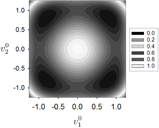
Figure 1: Contour plot depicting the shape of the $\rm Z_{2}$ invariant 2HDM potential ${\rm V}$ for the parameter set $\{\mu_{1}^{2},\mu_{2}^{2},\lambda_{1},\lambda_{2},\lambda_{345}\}=\{1,1,1,1,1\}$, in arbitrary mass units and normalized such that ${\rm V}_{\rm min}=0$. The four degenerate and disconnected global minima are shown in black around the central local maximum. The four minima form two pairs; the members within each pair are related by the $\mathrm{Z}_{2}$ symmetry and the two pairs are related to one another by ${\rm U}(1)_{\rm Y}$.

To determine whether the above extremal solutions represent local minima as well, we require that the Hessian ${\rm H}$ in (3.7), evaluated at the extremal points, is positive definite. This requirement generates two conditions:

$$\lambda_{1}\,\left(\frac{4\lambda_{2}\mu_{1}^{2}-2\lambda_{345}\mu_{2}^{2}}{4\lambda_{1}\lambda_{2}-\lambda_{345}^{2}}\right)\ >\ 0\;,$$ (3.14a)

$$\frac{\Big{(}4\lambda_{2}\mu_{1}^{2}-2\lambda_{345}\mu_{2}^{2}\Big{)}\,\Big{(}4\lambda_{1}\mu_{2}^{2}-2\lambda_{345}\mu_{1}^{2}\Big{)}}{4\lambda_{1}\lambda_{2}-\lambda_{345}^{2}}\ >\ 0\;.$$ (3.14b)

These two inequalities are equivalent to the positivity conditions for the squared VEVs in (3.11a) and (3.11b), provided $4\lambda_{1}\lambda_{2}>\lambda_{345}^{2}$ and $\lambda_{1}>0$. The constraint $\lambda_{1}>0$ represents one of the convexity conditions for the ${\rm Z}_{2}$-symmetric 2HDM potential (see Table 5). However, the restriction $4\lambda_{1}\lambda_{2}>\lambda_{345}^{2}$ has not been accounted before and creates two additional inequalities from the numerators of the fractions given in (3.11a) and (3.11b). These can be summarized in the double inequality

$$\frac{\lambda_{345}}{2\lambda_{2}}\ <\ \frac{\mu_{1}^{2}}{\mu_{2}^{2}}\ <\ \frac{2\lambda_{1}}{\lambda_{345}}\ .$$ (3.15)

Comparing this double inequality with the second line in Table 7, we see that local minima with $v^{0}_{1,2}=0$ and $v^{0}_{1,2}\neq 0$ cannot coexist. The value of the potential at the local minimum associated with the Lagrange multiplier $\zeta_{1,\,-}$ is given by

$$\mathrm{V}_{0}\ =\ \frac{\lambda_{345}\mu_{1}^{2}\mu_{2}^{2}-\lambda_{1}\mu_{2}^{4}-\lambda_{2}\mu_{1}^{4}}{4\lambda_{1}\lambda_{2}-\lambda_{345}^{2}}\ .$$ (3.16)

The corresponding value ${\rm V}_{0}$ for the local minimum related to $\zeta_{1,+}=-\lambda_{4}+\lambda_{5}$ is obtained by making the substitution $\lambda_{345}\to\bar{\lambda}_{345}$ in (3.16). Between these two solutions, the lowest minimum is given by $\zeta_{1,+}=-\lambda_{4}+\lambda_{5}$, if $\lambda_{5}>0$, and by $\zeta_{1,-}=-\lambda_{4}-\lambda_{5}$, if $\lambda_{5}<0$. Hence, the potential at the lowest minimum is given by

$$\mathrm{V}_{0}\ =\ \frac{\left(\lambda_{3}+\lambda_{4}-|\lambda_{5}|\right)\mu_{1}^{2}\mu_{2}^{2}-\lambda_{1}\mu_{2}^{4}-\lambda_{2}\mu_{1}^{4}}{4\lambda_{1}\lambda_{2}-\left(\lambda_{3}+\lambda_{4}-|\lambda_{5}|\right)^{2}}\ .$$ (3.17)

Note that this lowest minimum becomes a global one of the ${\rm Z}_{2}$-symmetric 2HDM potential, if (3.15) is fulfilled. Otherwise, the global minimum is given by (3.8). A numerical example of a ${\rm Z}_{2}$-symmetric 2HDM potential, where both $v^{0}_{1,2}$ are non-zero, is shown in Figure 1.

3.1.2 $\mathrm{Z}_{2}$ Topology

It is now important to determine the topology of the vacuum manifold for the $\mathrm{Z}_{2}$ invariant 2HDM potential, applying some of the general results presented in Section 2.3. In the symmetric phase, the $\mathrm{Z}_{2}$ invariant 2HDM potential is governed by the total symmetry group $\mathrm{G}_{\mathrm{Z}_{2}}\equiv\mathrm{Z}_{2}\otimes\mathrm{SU}(2)_{\mathrm{L}}\otimes\mathrm{U}(1)_{\mathrm{Y}}$, including the electroweak gauge group. After spontaneous symmetry breaking of the electroweak gauge group, we have

$$\mathrm{SU}(2)_{\mathrm{L}}\otimes\mathrm{U}(1)_{\mathrm{Y}}\simeq S^{\prime 3}\times S^{\prime 1}\ \to\ {\rm U(1)}_{\rm em}\simeq S^{1}\;.$$ (3.18)

In the above, we used the well-known homeomorphisms between compact groups and $n$-spheres denoted as $S^{n}$ (or $S^{\prime n}$): ${\rm U(1)}\simeq S^{1}$ and ${\rm SU(2)}\simeq S^{3}$. According to our discussion in Section 2.3, in the absence of any HF/CP symmetry in the theory, the vacuum manifold of the 2HDM will then be homeomorphic to the coset space $(S^{\prime 3}\times S^{\prime 1})/S^{1}$, which in turn is homeomorphic to $S^{3}$, i.e. $(S^{\prime 3}\times S^{\prime 1})/S^{1}~{}\simeq~{}S^{3}$.

In the present case, there exists an additional discrete $\mathrm{Z}_{2}$ symmetry acting on the 2HDM, which can break to the identity, i.e. $\mathrm{Z}_{2}\to{\bf I}$, after electroweak symmetry breaking. If this happens, the breaking pattern of the total symmetry group proceeds as follows:

$$\mathrm{G}_{\mathrm{Z}_{2}}\ \equiv\ \mathrm{Z}_{2}\otimes\mathrm{SU}(2)_{\mathrm{L}}\otimes\mathrm{U}(1)_{\mathrm{Y}}\ \to\ \mathrm{H}_{\mathrm{Z}_{2}}\ \equiv\ {\bf I}\otimes\mathrm{U}(1)_{\mathrm{em}}\;.$$ (3.19)

As a consequence, the topology of the vacuum manifold will then be described by the coset space ${\cal M}^{\mathrm{Z}_{2}}_{\Phi}=\mathrm{G}_{\mathrm{Z}_{2}}/\mathrm{H}_{\mathrm{Z}_{2}}$.

In order to generate the complete set ${\cal M}^{\mathrm{Z}_{2}}_{\Phi}$ of the vacuum manifold points in the $\Phi$-space, we first need to find an initial point $\Phi_{0}$ of the Majorana scalar-field multiplet, which remains invariant under the little group $\mathrm{H}_{\mathrm{Z}_{2}}$. Then, ${\cal M}^{\mathrm{Z}_{2}}_{\Phi}$ will be generated by the transitive action of $\mathrm{G}_{\mathrm{Z}_{2}}$ on $\Phi_{0}$. In the parameterization of the Higgs-doublet VEVs ${\rm V}_{1,2}$ of (2.42c) and (2.42f), the Majorana scalar-field vacuum point $\Phi_{0}$, which is invariant under $\mathrm{H}_{\mathrm{Z}_{2}}\cong{\rm U(1)}_{\rm em}$, is given by $v^{+}_{2}=0$ and $\xi=0$.

Let us first consider the non-trivial case where $v^{0}_{1,2}\neq 0$ as discussed in Section 3.1.1. The general vacuum manifold point $\Phi$ is given by

$$\Phi\ =\ {\cal M}^{\rm Z_{2}}_{+}\,\Phi_{0}\;,$$ (3.20)

where the HF transformation matrix ${\cal M}^{\rm Z_{2}}_{+}$ is stated in (2.51a) and ${\cal T}_{+}=\mathrm{T}_{+}=\{\sigma^{0}\,,\,\sigma^{3}\}$ are the $2\times 2$ HF transformation matrices given in Table 2 under the ${\rm Z}_{2}$ symmetry. It is interesting to see the different roles of the $\mathrm{Z}_{2}$ symmetry and the ${\rm U(1)_{Y}}$ hypercharge symmetry, according to the more intuitive chart:

$$\begin{array}[]{ccc}\left(\begin{array}[]{c}\mathbf{V}_{1}\\ \vskip 6.0pt plus 2.0pt minus 2.0pt\cr\mathbf{V}_{2}\end{array}\right)&\stackrel{{\scriptstyle\mathrm{U}(1)_{\mathrm{Y}}}}{{\longleftrightarrow}}&\left(\begin{array}[]{c}-\mathbf{V}_{1}\\ \vskip 6.0pt plus 2.0pt minus 2.0pt\cr-\mathbf{V}_{2}\end{array}\right)\\ \vskip 6.0pt plus 2.0pt minus 2.0pt\cr\mathrm{Z}_{2}\updownarrow&&\updownarrow\mathrm{Z}_{2}\\ \vskip 6.0pt plus 2.0pt minus 2.0pt\cr\left(\begin{array}[]{c}\mathbf{V}_{1}\\ \vskip 6.0pt plus 2.0pt minus 2.0pt\cr-\mathbf{V}_{2}\end{array}\right)&\stackrel{{\scriptstyle\mathrm{U}(1)_{\mathrm{Y}}}}{{\longleftrightarrow}}&\;\left(\begin{array}[]{c}-\mathbf{V}_{1}\\ \vskip 6.0pt plus 2.0pt minus 2.0pt\cr\mathbf{V}_{2}\end{array}\right)\;.\end{array}$$ (3.21)

Observe that for ${\rm Z}_{2}$-symmetric 2HDM scenarios with two non-zero VEVs $v^{0}_{1,2}\neq 0$, we cannot move via a ${\rm U}(1)_{\rm Y}$ transformation from one vacuum configuration, e.g. $(v^{0}_{1}\,,\,v^{0}_{2})$, to its ${\rm Z}_{2}$-symmetric one, i.e. $(v^{0}_{1}\,,\,-v^{0}_{2})$ or $(-v^{0}_{1}\,,\,v^{0}_{2})$. However, if $v^{0}_{1}$ or $v^{0}_{2}$ were zero, then such a transformation would be possible, and the discrete vacua will be connected via a continuous ${\rm U}(1)_{\rm Y}$ gauge transformation. In the latter case, there are no topological defects, such as domain walls or superconducting condensates similar to the ones discussed by Hodges [51], even though such scenarios might be interesting as they predict stable scalars which may act as DM (see, e.g. [40]).

On the other hand, the $\mathrm{Z}_{2}$ invariant 2HDM, where the two VEVs are non-zero, can lead to non-trivial topological solutions, such as domain walls . The vacuum manifold in the $\Phi$-space may be given by

$$\mathcal{M}^{\mathrm{Z}_{2}}_{\Phi}\ \simeq\ \mathrm{Z}_{2}\times S^{3}\;,$$ (3.22)

where the second factor $S^{3}$ comes from the breaking pattern of the electroweak gauge group as given in (3.18). Thus, the action of the zeroth homotopy group on this vacuum manifold is non-trivial, since $\Pi_{0}\left[\mathrm{Z}_{2}\times S^{3}\right]=\Pi_{0}\left[\mathrm{Z}_{2}\right]\times\Pi_{0}\left[S^{3}\right]\neq{\bf I}$, with $\Pi_{0}\left[S^{3}\right]={\bf I}$ [53]. This leaves the possibility for the formation of domain walls in the $\mathrm{Z}_{2}$ symmetric 2HDM, whose spatial profile is studied in Section 5.

3.2 U$(1)_{\mathrm{PQ}}$ Symmetry

We now analyze the Peccei–Quinn symmetry of the 2HDM, which is defined by the following transformations of the two Higgs doublets $\phi_{1,2}$:

$$\phi_{1} \to \phi^{\prime}_{1}\ =\ e^{-i\alpha}\,\phi_{1}\;,$$

$$\phi_{2} \to \phi^{\prime}_{2}\ =\ e^{i\alpha}\,\phi_{2}\;,$$

where $\alpha\in[0,\pi)$. The study of the neutral vacuum solutions of the U$(1)_{\mathrm{PQ}}$ invariant 2HDM proceeds in a very analogous fashion to the $\mathrm{Z}_{2}$ invariant 2HDM discussed in the previous section, since the only additional parameter restriction in the U$(1)_{\mathrm{PQ}}$ invariant theory is that one now has $\lambda_{5}=0$. Therefore, we only quote a few key results here.

For neutral vacuum solutions resulting from a non-singular matrix $\mathrm{N}_{\mu\nu}$, the VEVs are given by (3.4a) and (3.4c), with $\lambda_{5}=0$, i.e.

$$\langle\phi_{1}^{\dagger}\phi_{1}\rangle\ =\ \frac{2\lambda_{2}\mu_{1}^{2}-(\lambda_{3}-\zeta)\mu_{2}^{2}}{4\lambda_{1}\lambda_{2}-(\lambda_{3}-\zeta)^{2}}\ >\ 0\;,$$ (3.23a)

$$\langle\phi_{2}^{\dagger}\phi_{2}\rangle\ =\ \frac{2\lambda_{1}\mu_{2}^{2}-(\lambda_{3}-\zeta)\mu_{1}^{2}}{4\lambda_{1}\lambda_{2}-(\lambda_{3}-\zeta)^{2}}\ >\ 0\;,$$ (3.23b)

$$\langle\phi_{1}^{\dagger}\phi_{2}\rangle\ =\ \langle\phi_{2}^{\dagger}\phi_{1}\rangle\ =\ 0\;.$$ (3.23c)

There are two Lagrange multiplier solutions for this situation which are given by (3.6a) and (3.6b). Because of this close similarity, the vacuum manifold parameters are exactly the same as those detailed in Table 6 of Section 3.1. Correspondingly, the conditions for each solution to correspond to a minima are given in Table 7. As in the $\mathrm{Z}_{2}$ case, the U$(1)_{\mathrm{PQ}}$-invariant 2HDM must also have at least one doublet with a zero VEV, when $\mathrm{det}[\mathrm{N}_{\mu\nu}]\neq 0$, which only leads to topologically trivial configurations. We are, therefore, only interested in neutral vacuum solutions for which the matrix $\mathrm{N}_{\mu\nu}$ is singular.

3.2.1 Neutral Vacuum Solutions from a Singular Matrix N

In order for the matrix $\mathrm{N}_{\mu\nu}$ to have no inverse in the case of the Peccei-Quinn symmetry, we require that the expression given in (3.1) with $\lambda_{5}=0$ be equal to zero. This requirement leads to two candidate solutions:

$$\zeta_{1}\ =\ -\lambda_{4}\;,$$ (3.24a)

$$\zeta_{2,\pm}\ =\ \pm 2\sqrt{\lambda_{1}\lambda_{2}}+\lambda_{3}\;.$$ (3.24b)

However, for the same reasons as in the ${\rm Z}_{2}$ case, we have to reject the second solution $\zeta_{2,\pm}$, as it leads to an incompatible matrix equation, unless there is a particular fine-tuned relation between the parameters of the 2HDM. Therefore, we only focus on the first solution $\zeta_{1}$.

Under this choice for the Lagrange multiplier both $\mathrm{R}^{1}$ and $\mathrm{R}^{2}$ remain undetermined, since the $2\times 2$ matrix in (3.2n) becomes the null matrix. The remaining components of the vector $\mathrm{R}^{\mu}$ are found using (3.2g) and have the form:

$$\mathrm{R}^{0}\ =\ \frac{2\lambda_{1}\mu_{2}^{2}+2\lambda_{1}\mu_{1}^{2}-\lambda_{34}(\mu_{1}^{2}+\mu_{2}^{2})}{4\lambda_{1}\lambda_{2}-\lambda_{34}^{2}}\ ,$$ (3.25a)

$$\mathrm{R}^{3}\ =\ \frac{2\lambda_{2}\mu_{1}^{2}-2\lambda_{2}\mu_{2}^{2}+\lambda_{34}(\mu_{1}^{2}-\mu_{2}^{2})}{4\lambda_{1}\lambda_{2}-\lambda_{34}^{2}}\ .$$ (3.25b)

From these expressions, we obtain by means of (2.3) the VEVs of the scalar-field bilinears

$$\langle\phi_{1}^{\dagger}\phi_{1}\rangle\ =\ \frac{2\lambda_{2}\mu_{1}^{2}-\lambda_{34}\mu_{2}^{2}}{4\lambda_{1}\lambda_{2}-\lambda_{34}^{2}}\ \geq\ 0\;,$$ (3.26a)

$$\langle\phi_{2}^{\dagger}\phi_{2}\rangle\ =\ \frac{2\lambda_{1}\mu_{2}^{2}-\lambda_{34}\mu_{1}^{2}}{4\lambda_{1}\lambda_{2}-\lambda_{34}^{2}}\ \geq\ 0\;.$$ (3.26b)

For a neutral vacuum solution we require, as before, that $\mathrm{R}^{\mu}$ satisfies $\mathrm{R}_{\mu}\mathrm{R}^{\mu}=0$, which leads to the relation:

$$(\mathrm{R}^{1})^{2}+(\mathrm{R}^{2})^{2}\ =\ \frac{4\left(2\lambda_{2}\mu_{1}^{2}-\lambda_{34}\mu_{2}^{2}\right)\left(2\lambda_{1}\mu_{2}^{2}-\lambda_{34}\mu_{1}^{2}\right)}{\left(4\lambda_{1}\lambda_{2}-\lambda_{34}^{2}\right)^{2}}\ .$$ (3.27)

Employing the parameterization of ${\rm R}^{\mu}$ in (2.43), we find that the vacuum manifold parameters for the Lagrange multiplier $\zeta_{1}$ with $v_{2}^{+}=0$ are:

$$v_{1}^{0}\ =\ \sqrt{\frac{4\lambda_{2}\mu_{1}^{2}-2\lambda_{34}\mu_{2}^{2}}{4\lambda_{1}\lambda_{2}-\lambda_{34}^{2}}}\ ,$$ (3.28a)

$$v_{2}^{0}\ =\ \sqrt{\frac{4\lambda_{1}\mu_{2}^{2}-2\lambda_{34}\mu_{1}^{2}}{4\lambda_{1}\lambda_{2}-\lambda_{34}^{2}}}\ ,$$ (3.28b)

$$\xi\ \in\ [0,2\pi)\;.$$ (3.28c)

Notice that the phase $\xi$ remains undetermined, signifying the presence of a massless Goldstone boson, the so-called PQ axion [54, 55].

The conditions for a global minimum are identical to those of the ${\rm Z}_{2}$ case with $\lambda_{5}=0$. Thus, we have a global minimum with $v^{0}_{1,2}\neq 0$, provided

$$\frac{\lambda_{34}}{2\lambda_{2}}\ <\ \frac{\mu_{1}^{2}}{\mu_{2}^{2}}\ <\ \frac{2\lambda_{1}}{\lambda_{34}}\ .$$ (3.29)

The value of the U$(1)_{\mathrm{PQ}}$-invariant 2HDM potential at the global minimum is given by

$$\mathrm{V}_{0}\ =\ \frac{\lambda_{34}\mu_{1}^{2}\mu_{2}^{2}-\lambda_{1}\mu_{2}^{4}-\lambda_{2}\mu_{1}^{4}}{4\lambda_{1}\lambda_{2}-\lambda_{34}^{2}}\ .$$ (3.30)

As before, we find that neutral vacua where $v^{0}_{1,2}\neq 0$ and $v^{0}_{1}=0$ or $v^{0}_{2}=0$ cannot co-exist.

3.2.2 U$(1)_{\mathrm{PQ}}$ Topology

Let us now discuss the topology of the vacuum manifold associated with the U$(1)_{\mathrm{PQ}}$-invariant 2HDM potential. The total symmetry group of the potential in the symmetric phase is $\mathrm{G}_{\mathrm{U}(1)_{\mathrm{PQ}}}=\mathrm{U}(1)_{\mathrm{PQ}}\otimes\mathrm{SU}(2)_{\mathrm{L}}\otimes\mathrm{U}(1)_{\mathrm{Y}}$. After electroweak symmetry breaking [cf. (3.18)], the U$(1)_{\mathrm{PQ}}$ symmetry breaks into the identity ${\bf I}$, so the unbroken group is $\mathrm{H}_{\mathrm{U}(1)_{\mathrm{PQ}}}={\bf I}\otimes\mathrm{U}(1)_{\mathrm{em}}$. As a consequence, the vacuum manifold in the $\Phi$-space is given by the set

$$\mathcal{M}^{\mathrm{U(1)}_{\mathrm{PQ}}}_{\Phi}\ =\ \mathrm{G}_{\mathrm{U}(1)_{\mathrm{PQ}}}/\mathrm{H}_{\mathrm{U}(1)_{\mathrm{PQ}}}\ \simeq\ S^{1}\times S^{3}\;,$$ (3.31)

where we used the fact that U$(1)_{\mathrm{PQ}}$ is homeomorphic to $S^{1}$. We now observe that the first homotopy group of this vacuum manifold is non-trivial, i.e. $\Pi_{1}\left[S^{1}\times S^{3}\right]=\Pi_{1}\left[S^{1}\right]\times\Pi_{1}\left[S^{3}\right]=\Pi_{1}\left[S^{1}\right]=\mathbb{Z}\neq{\bf I}$, since $\Pi_{1}\left[S^{3}\right]={\bf I}$. This implies that the U$(1)_{\mathrm{PQ}}$-invariant 2HDM has a string or vortex solution, which we analyze in Section 5.

It is interesting to discuss the construction of the vacuum manifold in the $\Phi$-space. As stated in (2.51a), a general point of the vacuum manifold is given by $\Phi\ =\ \mathcal{M}^{\mathrm{U(1)}_{\mathrm{PQ}}}_{+}\,\Phi_{0}$, where $\Phi_{0}$ is defined in terms of the non-zero VEVs $v^{0}_{1,2}$ given in (3.28a) and (3.28b) and by setting $\xi=0$. Moreover, in the 8-dimensional Majorana $\Phi$-space, the HF transformation matrix $\mathcal{M}^{\mathrm{U(1)}_{\mathrm{PQ}}}_{+}$ takes on the form:

$$\mathcal{M}^{\mathrm{U(1)}_{\mathrm{PQ}}}_{+} = \left(\frac{\sigma^{0}+\sigma^{3}}{2}\right)\otimes\mathcal{T}_{+}\otimes\mathrm{U}_{+}(\tilde{\theta}^{1},\tilde{\theta}^{2},\theta_{-})\>+\>\left(\frac{\sigma^{0}-\sigma^{3}}{2}\right)\otimes\mathcal{T}^{*}_{+}\otimes\mathrm{U}_{-}(\tilde{\theta}^{1},\tilde{\theta}^{2},\theta_{-})$$

$$= \left(\frac{\sigma^{0}+\sigma^{3}}{2}\right)\otimes\exp\left[\,2i\alpha\left(\frac{\sigma^{0}-\sigma^{3}}{2}\right)\right]\otimes\mathrm{U}_{+}(\tilde{\theta}^{1},\tilde{\theta}^{2},\theta_{-}-\alpha)$$

$$+\ \left(\frac{\sigma^{0}-\sigma^{3}}{2}\right)\otimes\exp\left[\,-2i\alpha\left(\frac{\sigma^{0}-\sigma^{3}}{2}\right)\right]\otimes\mathrm{U}_{-}(\tilde{\theta}^{1},\tilde{\theta}^{2},\theta_{-}-\alpha)\;.$$

Here, we have explicitly displayed the dependence of the gauge-group factors ${\rm U}_{\pm}$ on their group parameters and made use of the fact that the HF transformation matrix $\mathcal{T}_{+}=e^{-i\alpha\sigma_{3}}$ for the PQ symmetry may be written as $\mathcal{T}_{+}=e^{-i\alpha}e^{i\alpha(\sigma^{0}-\sigma^{3})}$. We may now re-define the group parameter $\theta_{-}$ as $\tilde{\theta}_{-}=\theta_{-}-\alpha\in[0,2\pi)$, and so having the group parameter $2\alpha\in[0,2\pi)$ to span now the complete space of the U(1)_PQ group. Note that this result is identical to the one that would be obtained in the ${\rm R}^{\mu}$ space, as can be easily deduced from Table 3.

3.3 SO$(3)_{\mathrm{HF}}$ Symmetry

An interesting HF symmetry emerges from the invariance of the 2HDM potential under a naive ${\rm SU(2)_{HF}}$ transformation of the Higgs fields, i.e.

$$\phi_{1} \to \phi^{\prime}_{1}\ =\ e^{-i\alpha}\cos\theta\,\phi_{1}\>+\>e^{-i\beta}\sin\theta\,\phi_{2}\;,$$

$$\phi_{2} \to \phi^{\prime}_{2}\ =\ -e^{i\beta}\sin\theta\,\phi_{1}\>+\>e^{i\alpha}\cos\theta\,\phi_{2}\;.$$

To avoid a double cover of the ${\rm SU(2)_{HF}}$ group because of the presence of ${\rm U(1)_{Y}}$ hypercharge rotations, we have to restrict the group parameters $\theta,\,\alpha,\,\beta$ to lie in the interval $[0,\pi)$. Hence, the actual HF symmetry is the coset group ${\rm SU(2)_{HF}}/{\rm Z_{2}}$ [23], which is isomorphic to ${\rm SO(3)_{HF}}$ in the field-bilinear ${\rm R}^{\mu}$ space. For this reason, this symmetry was called the ${\rm SO(3)_{HF}}$ symmetry.

The parameters of the 2HDM potential under the ${\rm SO(3)_{HF}}$ symmetry are restricted, as shown in Table 4. In fact, most of the results can be easily recovered from the ${\rm Z}_{2}$ case in Section 3.1, by making the replacements: $\lambda_{2}\to\lambda_{1}$, $\lambda_{4}\to 2\lambda_{1}-\lambda_{3}$, $\mu^{2}_{2}\to\mu^{2}_{1}$ and putting $\lambda_{5}=0$. Therefore, we will only report key intermediate results in this section. As before, we first assume that the inverse of $\mathrm{N}_{\mu\nu}$ exists, with the determinant of $\mathrm{N}_{\mu\nu}$ given by

$$\mathrm{det}[\mathrm{N}_{\mu\nu}]\ =\ \left(2\lambda_{1}+\lambda_{3}-\zeta\right)\,\left(2\lambda_{1}-\lambda_{3}+\zeta\right)^{3}\;.$$ (3.33)

Because of the more restrictive nature of the SO$(3)_{\mathrm{HF}}$ symmetry, the matrix equation $\mathrm{N}_{\mu\nu}\mathrm{R}^{\nu}=\mathrm{M}_{\mu}$ splits into four separate equations:

$$(2\lambda_{1}+\lambda_{3}-\zeta)\,\mathrm{R}^{0}\ =\ 2\mu_{1}^{2}\;,$$ (3.34a)

$$(2\lambda_{1}-\lambda_{3}+\zeta)\,\mathrm{R}^{1}\ =\ 0\;,$$ (3.34b)

$$(2\lambda_{1}-\lambda_{3}+\zeta)\,\mathrm{R}^{2}\ =\ 0\;,$$ (3.34c)

$$(2\lambda_{1}-\lambda_{3}+\zeta)\,\mathrm{R}^{3}\ =\ 0\;.$$ (3.34d)

On the basis of the above assumption that $\mathrm{N}_{\mu\nu}$ is invertible, the components of the 4-vector $\mathrm{R}^{\mu}$ are easily found to be

$$\mathrm{R}^{0}\ =\ \frac{2\mu_{1}^{2}}{2\lambda_{1}+\lambda_{3}-\zeta}\ ,$$ (3.35a)

$$\mathrm{R}^{1}\ =\ \mathrm{R}^{2}\ =\ \mathrm{R}^{3}\ =\ 0\;.$$ (3.35b)

On the other hand, the constraint for a neutral vacuum solution requires that ${\rm R}^{\mu}$ is a null vector, satisfying ${\rm R}_{\mu}{\rm R}^{\mu}=0$. Since all the “spatial” components ${\rm R}^{1,2,3}$ vanish, so should the “time” component, i.e. ${\rm R}^{0}=0$. This last result tells us that the Higgs doublets should have vanishing VEVs, i.e. $v^{0}_{1,2}=0$, leaving the electroweak gauge group unbroken. This is an unrealistic scenario and can only be obtained in the limit $\mu^{2}_{1}\to 0$, or $\zeta\to\pm\infty$. We will therefore investigate neutral vacuum solutions that result from a singular matrix ${\rm N}_{\mu\nu}$.

3.3.1 Neutral Vacuum Solutions from a Singular Matrix N

From (3.33), we readily see that the following choices of the Lagrange multiplier render $\mathrm{N}_{\mu\nu}$ singular:

$$\zeta_{1}\ =\ -2\lambda_{1}+\lambda_{3}\;,$$ (3.36a)

$$\zeta_{2}\ =\ 2\lambda_{1}+\lambda_{3}\;.$$ (3.36b)

However, from (3.34a), we notice that the solution $\zeta_{2}$ implies either $\mathrm{R}^{0}\to\infty$, or $\mu^{2}_{1}\to 0$, both of which lead to unrealistic scenarios of electroweak symmetry breaking. Therefore, we concentrate on the Lagrange multiplier solution $\zeta_{1}$.

Considering the Lagrange multiplier solution $\zeta_{1}$, we obtain from (3.34a) that

$$\mathrm{R}^{0}\ =\ \frac{\mu_{1}^{2}}{2\lambda_{1}}\ .$$ (3.37)

Instead, from (3.34b)–(3.34d), we see that all the “spatial components” ${\rm R}^{1,2,3}$ remain undetermined. The only constraint that can be placed upon the three “spatial” components of $\mathrm{R}^{\mu}$ is the requirement of a neutral vacuum solution, $\mathrm{R}_{\mu}\mathrm{R}^{\mu}=0$, which implies that

$$(\mathrm{R}^{1})^{2}+(\mathrm{R}^{2})^{2}+(\mathrm{R}^{3})^{2}\ =\ \frac{\mu_{1}^{4}}{4\lambda_{1}^{2}}\ .$$ (3.38)

In terms of the vacuum manifold parameters $v^{0}_{1,2}$ and $\xi$, (3.37) and (3.38) are translated into

$$v_{1}^{0}\ =\ \frac{\mu_{1}}{\sqrt{\lambda_{1}}}\ \sin\theta\;,\qquad v_{2}^{0}\ =\ \frac{\mu_{1}}{\sqrt{\lambda_{1}}}\ \cos\theta\;,$$ (3.39)

where $\xi\in[0,2\pi)$ and $\theta\in[0,\pi)$ remain undetermined. The latter signifies the presence of two Goldstone bosons. Specifically, the one associated with the phase $\xi$ is a CP-odd scalar, whereas the one related to the polar angle $\theta$ is a ‘CP-even’ boson. This result can be cross-checked independently from the explicit analytical expressions presented in [16] for the general Higgs-boson mass matrices. The global minimum of the SO$(3)_{\mathrm{HF}}$-symmetric 2HDM potential is given by

$$\mathrm{V}_{0}\ =\ -\;\frac{\mu_{1}^{4}}{4\lambda_{1}}\ .$$ (3.40)

Such a global minimum is always guaranteed, as long as $\mu^{2}_{1}$ is positive and the bounded-from-below condition, $2\lambda_{1}>|\lambda_{3}|$ given in Table 5 is satisfied.

3.3.2 SO$(3)_{\mathrm{HF}}$ Topology

It is interesting to analyze the topology of the vacuum manifold arising from the spontaneous symmetry breaking of an SO$(3)_{\mathrm{HF}}$-invariant 2HDM potential. In the symmetric phase of the theory, the SO$(3)_{\mathrm{HF}}$-invariant 2HDM potential has the symmetry, which is described by the group [23]

$$\mathrm{G}_{\mathrm{SO(3)}_{\mathrm{HF}}}\ =\ (\mathrm{SU(2)}_{\mathrm{HF}}/{\rm Z}_{2})\otimes\mathrm{SU}(2)_{\mathrm{L}}\otimes\mathrm{U}(1)_{\mathrm{Y}}\ \cong\ \mathrm{SO(3)}_{\mathrm{HF}}\otimes\mathrm{SU}(2)_{\mathrm{L}}\otimes\mathrm{U}(1)_{\mathrm{Y}}\;.$$ (3.41)

Using the results of the previous section, we see that out of the three generators of the SU$(2)_{\mathrm{HF}}/{\rm Z}_{2}$ group, one linear combination of generators, $(\sigma^{0}+\sigma^{3})/2$ related to a residual HF symmetry, which we call ${\rm U(1)}_{\rm HF}$, remains unbroken after the electroweak symmetry breaking, resulting in the little group

$$\mathrm{H}_{\mathrm{SO(3)}_{\mathrm{HF}}}\ =\ \mathrm{U(1)}_{\mathrm{HF}}\otimes\mathrm{SU}(2)_{\mathrm{L}}\otimes\mathrm{U}(1)_{\mathrm{Y}}\ \cong\ \mathrm{SO(2)}_{\mathrm{HF}}\otimes\mathrm{SU}(2)_{\mathrm{L}}\otimes\mathrm{U}(1)_{\mathrm{Y}}\;.$$ (3.42)

Then, the vacuum manifold $\mathcal{M}^{\mathrm{SO(3)}_{\mathrm{HF}}}_{\Phi}$ may be described by the product of spaces:

$$\mathcal{M}^{\mathrm{SO(3)}_{\mathrm{HF}}}_{\Phi}\ =\ \mathrm{G}_{\mathrm{SO(3)}_{\mathrm{HF}}}/\mathrm{H}_{\mathrm{SO(3)}_{\mathrm{HF}}}\ \simeq\ S^{2}\times S^{3}\;,$$ (3.43)

where the first factor $S^{2}$ is obtained using the known homeomorphism ${\rm SO(3)_{HF}/SO(2)_{HF}}$ $\simeq S^{2}$ and the second one $S^{3}$ is due to the breaking of the electroweak group to ${\rm U(1)}_{\rm em}$. We observe that the second homotopy group of $\mathcal{M}^{\mathrm{SO(3)}_{\mathrm{HF}}}_{\Phi}$ is non-trivial. More explicitly, $\Pi_{2}\left[S^{2}\times S^{3}\right]=\Pi_{2}\left[S^{2}\right]\times\Pi_{2}\left[S^{3}\right]=\Pi_{2}\left[S^{2}\right]\neq{\bf I}$, since $\Pi_{2}\left[S^{3}\right]={\bf I}$. Consequently, spontaneous symmetry breaking of the $\mathrm{SO(3)}_{\mathrm{HF}}$-symmetric 2HDM can give rise to global monopoles.

As with the previous HF symmetries, we are able to construct the entire vacuum manifold by the transitive action of the total group $\mathrm{G}_{\mathrm{SO(3)}_{\mathrm{HF}}}$ stated in (3.41) on the vacuum point $\Phi_{0}$, which remains invariant under the little group $\mathrm{H}_{\mathrm{SO(3)}_{\mathrm{HF}}}$ given in (3.42). An appropriate representation of $\Phi_{0}$ consistent with the latter property is given by the VEVs

$${\bf V}_{1}\ =\ \left(\begin{array}[]{c}0\\ \vskip 6.0pt plus 2.0pt minus 2.0pt\cr 0\end{array}\right)\;,\qquad{\bf V}_{2}\ =\ \frac{1}{\sqrt{2}}\left(\begin{array}[]{c}0\\ \vskip 6.0pt plus 2.0pt minus 2.0pt\cr\frac{\mu_{1}}{\sqrt{\lambda_{1}}}\end{array}\right)\;,$$ (3.44)

where we set $\theta=\xi=0$ in (3.39). The general point $\Phi$ on the vacuum manifold is then given by the action of the coset set of HF transformation matrices $\mathcal{M}^{\mathrm{SO(3)}_{\mathrm{HF}}}_{+}$ on $\Phi_{0}$, i.e. $\Phi=\mathcal{M}^{\mathrm{SO(3)}_{\mathrm{HF}}}_{+}\,\Phi_{0}$, where

$$\mathcal{M}^{\mathrm{SO(3)}_{\mathrm{HF}}}_{+}\ =\ \left(\frac{\sigma^{0}+\sigma^{3}}{2}\right)\otimes\mathcal{T}_{+}\otimes\mathrm{U}_{+}(\tilde{\theta}^{1},\tilde{\theta}^{2},\theta_{-})\>+\>\left(\frac{\sigma^{0}-\sigma^{3}}{2}\right)\otimes\mathcal{T}^{*}_{+}\otimes\mathrm{U}_{-}(\tilde{\theta}^{1},\tilde{\theta}^{2},\theta_{-})\;.$$ (3.45)

Here, the $2\times 2$ HF transformation matrices ${\cal T}_{+}$ belong to the coset space of the $\rm SO(3)_{HF}$ symmetry in the adjoint representation, i.e. ${\cal T}_{+}\in({\rm SU(2)}_{\rm HF}/{\rm Z_{2}})/{\rm U}(1)_{\rm HF}$, and can be represented as

$${\cal T}_{+}\ =\ \left(\begin{array}[]{cc}e^{-i\alpha}\cos\theta&e^{-i\beta}\sin\theta\\ \vskip 6.0pt plus 2.0pt minus 2.0pt\cr-e^{i\beta}\sin\theta&e^{i\alpha}\cos\theta\end{array}\right)\,\left(\begin{array}[]{cc}e^{i\chi}&0\\ \vskip 6.0pt plus 2.0pt minus 2.0pt\cr 0&1\end{array}\right)\ =\ e^{-i\beta}\,\left(\begin{array}[]{cc}\cos\theta&\sin\theta\\ \vskip 6.0pt plus 2.0pt minus 2.0pt\cr-e^{i(\alpha+\beta)}\sin\theta&e^{i(\alpha+\beta)}\cos\theta\end{array}\right)\;,$$ (3.46)

where we set the free ${\rm U}(1)_{\rm HF}$ phase $\chi$ to be $\chi=\alpha-\beta$, in obtaining the second equation. As in the PQ symmetry case, the overall factor $e^{-i\beta}$ can be absorbed into the definition of the gauge-group parameter $\theta_{-}$, i.e. by defining $\tilde{\theta}_{-}=\theta_{-}-\beta\in[0,2\pi)$. The HF transformation matrices $\mathcal{M}^{\mathrm{SO(3)}_{\mathrm{HF}}}_{+}$ can then be written down as

$$\mathcal{M}^{\mathrm{SO(3)}_{\mathrm{HF}}}_{+}\! = \!\left(\frac{\sigma^{0}+\sigma^{3}}{2}\right)\otimes\left(\begin{array}[]{cc}\cos\theta&\sin\theta\\ \vskip 6.0pt plus 2.0pt minus 2.0pt\cr-e^{i(\alpha+\beta)}\sin\theta&e^{i(\alpha+\beta)}\cos\theta\end{array}\right)\otimes\mathrm{U}_{+}(\tilde{\theta}^{1},\tilde{\theta}^{2},\tilde{\theta}_{-})$$ (3.49)

$$+ \!\!\left(\frac{\sigma^{0}-\sigma^{3}}{2}\right)\otimes\left(\begin{array}[]{cc}\cos\theta&\sin\theta\\ \vskip 6.0pt plus 2.0pt minus 2.0pt\cr-e^{-i(\alpha+\beta)}\sin\theta&e^{-i(\alpha+\beta)}\cos\theta\end{array}\right)\otimes\mathrm{U}_{-}(\tilde{\theta}^{1},\tilde{\theta}^{2},\tilde{\theta}_{-})\;.\qquad$$ (3.52)

If we ignore the $S^{3}$ gauge rotations by setting ${\rm U}_{\pm}=\sigma^{0}$, the action of $\mathcal{M}^{\mathrm{SO(3)}_{\mathrm{HF}}}_{+}$ on $\Phi_{0}$ then generates the general vacuum manifold point given in (3.39), with $\xi=\alpha+\beta\in[0,2\pi)$ and $\theta\in[0,\pi)$. Thus, the vacuum manifold of the SO(3)_HF-broken 2HDM is homeomorphic to $S^{2}$, parameterized by the azimuthal angle $\theta$ and the polar angle $\xi=\alpha+\beta$. This parameterization will be used in Section 5 to analyze the monopole solution in this model.

4 Neutral Vacuum Solutions of the CP Symmetries

In this section, we will study the three generic CP symmetries, termed CP1, CP2 and CP3. These three CP symmetries impose specific relations [23] among the parameters of the 2HDM potential, which are presented in Table 8.

Symmetry	$\mu_{1}^{2}$	$\mu_{2}^{2}$	$m_{12}^{2}$	$\lambda_{1}$	$\lambda_{2}$	$\lambda_{3}$	$\lambda_{4}$	$\lambda_{5}$	$\lambda_{6}$	$\lambda_{7}$
CP1	–	–	Real	–	–	–	–	Real	Real	Real
CP2	–	$\mu_{1}^{2}$	0	–	$\lambda_{1}$	–	–	–	–	$-\lambda_{6}$
CP3	–	$\mu_{1}^{2}$	0	–	$\lambda_{1}$	–	–	$2\lambda_{1}-\lambda_{3}-\lambda_{4}$	0	0

Table 8: Parameter relations in the 2HDM potential that result from the imposition of the three generic CP symmetries. A dash indicates the absence of a constraint.

Implementing the constraints on the potential parameters due to the CP symmetries, the four general convexity conditions (2.10a)–(2.10c) and (C.6) take on a simpler form. These four conditions are displayed in Table 9. In particular, for the CP3 case, the four convexity conditions are not all independent of each other, so only the two distinct conditions are presented.

Convexity
Condition	CP1	CP2	CP3
1	$\lambda_{1}+\lambda_{2}+\lambda_{3}>0$	$2\lambda_{1}>-\lambda_{3}$	$2\lambda_{1}>|\lambda_{3}|$
2	$\lambda_{4}>-\lambda_{5}+\frac{(\lambda_{6}+\lambda_{7})^{2}}{\lambda_{1}+\lambda_{2}+\lambda_{3}}$	$\lambda_{4}>-R_{5}$	$2\lambda_{4}>2\lambda_{1}-\lambda_{3}$
3	$\lambda_{4}>\lambda_{5}$	$\lambda_{4}^{2}>|\lambda_{5}|^{2}$	–
4	$\lambda_{1}\lambda_{2}-\frac{1}{4}\lambda_{3}^{2}>$	$2\lambda_{1}-\lambda_{3}>$	–
	$\frac{\lambda_{1}\lambda_{6}^{2}+\lambda_{2}\lambda_{7}^{2}-\lambda_{3}\lambda_{6}\lambda_{7}}{\lambda_{4}+\lambda_{5}}$	$\frac{4|\lambda_{6}|^{2}(\lambda_{4}-R_{5})-8I_{6}(I_{5}R_{6}-R_{5}I_{6})}{\lambda_{4}^{2}-|\lambda_{5}|^{2}}$

Table 9: The four convexity conditions for a bounded-from-below 2HDM potential for each of the three CP symmetries. A dash signifies the absence of any additional constraint.

As in the previous section, our aim is to derive analytical expressions for the neutral VEVs of $\phi_{1,2}$ in terms of the 2HDM potential parameters for each of the three CP symmetries, by making use of the Lagrange multiplier method. These results will be used to determine the existence and the nature of possible topological defects which will be discussed in detail in Section 5.

4.1 CP1 Symmetry

The discrete CP1 symmetry of the 2HDM represents the standard CP transformation of the two Higgs doublets $\phi_{1,2}$, given by

$$\phi_{1} \to \phi^{\prime}_{1}\ =\ \phi_{1}^{*}\;,$$

$$\phi_{2} \to \phi^{\prime}_{2}\ =\ \phi_{2}^{*}\;.$$

Taking into account the CP1 parameter restrictions of Table 8, we calculate the VEVs of $\phi_{1,2}$ by imposing the extremization condition (2.9a) and the condition (2.9b) for an electrically neutral vacuum. As before, we consider two cases: (i) $\mathrm{det}[\mathrm{N}_{\mu\nu}]\neq 0$ and (ii) $\mathrm{det}[\mathrm{N}_{\mu\nu}]=0$.

The determinant of $\mathrm{N}_{\mu\nu}$ resulting from a CP1-invariant 2HDM potential follows from Appendix C and can be expressed in the factorized form:

$$\mathrm{det}[\mathrm{N}_{\mu\nu}]\ =\ (\bar{\lambda}_{45}+\zeta)\left[\left(\lambda_{45}+\zeta\right)\left(4\lambda_{1}\lambda_{2}-(\lambda_{3}-\zeta)^{2}\right)-4\lambda_{1}\lambda_{6}^{2}-4\lambda_{2}\lambda_{7}^{2}+4\lambda_{6}\lambda_{7}(\lambda_{3}-\zeta)\right]\;.$$ (4.1)

Moreover, the extremization condition $\mathrm{N}_{\mu\nu}\mathrm{R}^{\nu}=\mathrm{M}_{\mu}$ decomposes into two equations:

$$\left(\begin{array}[]{ccc}\lambda_{1}\!+\!\lambda_{2}\!+\!\lambda_{3}\!-\!\zeta&\lambda_{6}\!+\!\lambda_{7}&\lambda_{1}\!-\!\lambda_{2}\\ \vskip 6.0pt plus 2.0pt minus 2.0pt\cr\lambda_{6}\!+\!\lambda_{7}&\lambda_{4}\!+\!\lambda_{5}\!+\!\zeta&\lambda_{6}\!-\!\lambda_{7}\\ \vskip 6.0pt plus 2.0pt minus 2.0pt\cr\lambda_{1}\!-\!\lambda_{2}&\lambda_{6}\!-\!\lambda_{7}&\lambda_{1}\!+\!\lambda_{2}\!-\!\lambda_{3}\!+\!\zeta\end{array}\right)\!\!\left(\begin{array}[]{c}\mathrm{R}^{0}\\ \vskip 6.0pt plus 2.0pt minus 2.0pt\cr\mathrm{R}^{1}\\ \vskip 6.0pt plus 2.0pt minus 2.0pt\cr\mathrm{R}^{3}\end{array}\right)\ =\ \left(\begin{array}[]{c}\mu_{1}^{2}+\mu_{2}^{2}\\ \vskip 6.0pt plus 2.0pt minus 2.0pt\cr 2m_{12}^{2}\\ \vskip 6.0pt plus 2.0pt minus 2.0pt\cr\mu_{1}^{2}-\mu_{2}^{2}\end{array}\right)\;,$$ (4.2j)

$$(\lambda_{4}-\lambda_{5}+\zeta)\,\mathrm{R}^{2}\ =\ 0\;.$$ (4.2k)

Assuming that the matrix $\mathrm{N}_{\mu\nu}$ is invertible, we observe that $\mathrm{R}^{2}=0$, which implies that $\langle\phi_{1}^{\dagger}\phi_{2}\rangle=\langle\phi_{2}^{\dagger}\phi_{1}\rangle$. This latter condition can be satisfied in two ways, if $v^{0}_{2}\neq 0$. The first possibility is to have $\xi=0$, which amounts to the non-breaking of the CP1 symmetry by the vacuum. The second possibility is to have $v^{0}_{1}=0$, with $\xi\neq 0$ and possibly $v^{+}_{2}\neq 0$. However, $\xi$ and $v^{+}_{2}$ can be set to zero by an SU$(2)_{\rm L}$ gauge rotation, giving rise to a CP1-invariant vacuum. Hence, the neutral vacuum solutions arising from an invertible matrix $\mathrm{N}_{\mu\nu}$ do not break the discrete CP1 symmetry and so do not lead to topological defects, such as domain walls. We therefore turn our attention to situations where the determinant of the matrix $\mathrm{N}_{\mu\nu}$ is singular, thanks to specific choices of the Lagrange multiplier $\zeta$.

4.1.1 Neutral Vacuum Solutions from a Singular Matrix N

In order for the matrix $\mathrm{N}_{\mu\nu}$ to have no inverse under the CP1 symmetry, we require that the determinant of $\rm N_{\mu\nu}$ vanishes. This is guaranteed by setting the the expression in (4.1) to zero. We find four possible solutions for the Lagrange multiplier, three attributed to (4.2j) and one attributed to (4.2k). However, as we have previously seen for the other symmetries studied so far, since the RHS of (4.2j) is in general a non-zero vector in this case, unless $\mu^{2}_{1}=\mu^{2}_{2}=0$ and $\mathrm{Re}(m_{12}^{2})=0$, this matrix equation is overdetermined. Unless the parameters $\mu^{2}_{1,2}$, $\mathrm{Re}(m_{12}^{2})$ and the quartic couplings $\lambda_{1,2,\dots,7}$ satisfy an unnatural fine-tuning relation, the matrix equation (4.2j) becomes incompatible for the Lagrange multipliers that result from requiring that the matrix of (4.2j) is singular. We therefore reject these three possible Lagrange multipliers and focus on the single Lagrange multiplier solution to (4.2k):

$$\zeta\ =\ -\bar{\lambda}_{45}\;.$$ (4.3)

This choice of $\zeta$ lifts the constraint $\mathrm{R}^{2}=0$, which resulted from a non-singular matrix $\mathrm{N}_{\mu\nu}$. As consequence, the CP-odd phase $\xi$ can be non-zero in general, thus triggering spontaneous breakdown of the CP1 symmetry after the electroweak symmetry breaking. This phenomenon is called spontaneous CP violation in the literature [20, 36].

Substituting the value of the Lagrange multiplier $\zeta$ in (4.3) into the matrix equation (4.2j), we can calculate the individual components of the 4-vector $\mathrm{R}^{\mu}$. These are given by

$$\mathrm{R}^{0}\ =\ \frac{1}{\rm A}\,\Big{\{}\left[\lambda_{5}(2\lambda_{2}-\bar{\lambda}_{345})+\bar{\lambda}_{67}\lambda_{7}\right]\mu_{1}^{2}+\left[\lambda_{5}(2\lambda_{1}-\bar{\lambda}_{345})-\lambda_{6}\bar{\lambda}_{67}\right]\mu_{2}^{2}$$

$$\hskip 42.67912pt+\,\left[\bar{\lambda}_{12}\bar{\lambda}_{67}-(\lambda_{12}\!-\!\bar{\lambda}_{345})\lambda_{67}\right]m_{12}^{2}\Big{\}}\;,$$ (4.4a)

$$\mathrm{R}^{1}\ =\ \frac{1}{\rm A}\,\Big{\{}\left(\bar{\lambda}_{345}\lambda_{7}-2\lambda_{2}\lambda_{6}\right)\mu_{1}^{2}+\left(\bar{\lambda}_{345}\lambda_{6}-2\lambda_{1}\lambda_{7}\right)\mu_{2}^{2}+\left(4\lambda_{1}\lambda_{2}-\bar{\lambda}_{345}^{2}\right)m_{12}^{2}\,\Big{\}}\;,$$ (4.4b)

$$\mathrm{R}^{3}\ =\ \frac{1}{\rm A}\,\Big{\{}\left[\lambda_{5}(2\lambda_{2}+\bar{\lambda}_{345})-\lambda_{67}\lambda_{7}\right]\mu_{1}^{2}+\left[\lambda_{6}\lambda_{67}-\lambda_{5}(2\lambda_{1}+\bar{\lambda}_{345})\right]\mu_{2}^{2}$$

$$\hskip 42.67912pt+\,\left[\bar{\lambda}_{12}\lambda_{67}-(\lambda_{12}+\bar{\lambda}_{345})\bar{\lambda}_{67})\right]m_{12}^{2}\,\Big{\}}\,,$$ (4.4c)

with

$$\mathrm{A}\ =\ \lambda_{5}\left(4\lambda_{1}\lambda_{2}-\bar{\lambda}_{345}^{2}\right)-2\lambda_{1}\lambda_{7}^{2}-2\lambda_{2}\lambda_{6}^{2}+2\bar{\lambda}_{345}\lambda_{6}\lambda_{7}\;.$$ (4.5)

From (4.4a) and (4.4c), we can now calculate, by means of (2.3), the VEVs for the bilinear field expressions:

$$\langle\phi_{1}^{\dagger}\phi_{1}\rangle\ =\ \frac{\left(2\lambda_{2}\lambda_{5}-\lambda_{7}^{2}\right)\mu_{1}^{2}+\left(\lambda_{6}\lambda_{7}-\bar{\lambda}_{345}\lambda_{5}\right)\mu_{2}^{2}+\left(\bar{\lambda}_{345}\lambda_{7}-2\lambda_{2}\lambda_{6}\right)m_{12}^{2}}{\lambda_{5}\left(4\lambda_{1}\lambda_{2}-\bar{\lambda}_{345}^{2}\right)-2\lambda_{1}\lambda_{7}^{2}-2\lambda_{2}\lambda_{6}^{2}+2\bar{\lambda}_{345}\lambda_{6}\lambda_{7}}\ >\ 0\;,$$ (4.6a)

$$\langle\phi_{2}^{\dagger}\phi_{2}\rangle\ =\ \frac{\left(\lambda_{6}\lambda_{7}-\bar{\lambda}_{345}\lambda_{5}\right)\mu_{1}^{2}+\left(2\lambda_{1}\lambda_{5}-\lambda_{6}^{2}\right)\mu_{2}^{2}+\left(\bar{\lambda}_{345}\lambda_{6}-2\lambda_{1}\lambda_{7}\right)m_{12}^{2}}{\lambda_{5}\left(4\lambda_{1}\lambda_{2}-\bar{\lambda}_{345}^{2}\right)-2\lambda_{1}\lambda_{7}^{2}-2\lambda_{2}\lambda_{6}^{2}+2\bar{\lambda}_{345}\lambda_{6}\lambda_{7}}\ >\ 0\;.$$ (4.6b)

In order to fix the remaining undetermined component $\mathrm{R}^{2}$, we impose the neutral vacuum condition (2.9b) on the 4-vector $\mathrm{R}^{\mu}$, i.e. $\mathrm{R}^{\mu}$ has to be a null vector. In this way, we find for the second component $\mathrm{R}^{2}$ that

$$\mathrm{R}^{2}\!\! = \!\!\pm\frac{1}{\mathrm{A}}\;\bigg{\{}\,4\Big{[}\left(2\lambda_{2}\lambda_{5}-\lambda_{7}^{2}\right)\mu_{1}^{2}+\left(\lambda_{6}\lambda_{7}-\bar{\lambda}_{345}\lambda_{5}\right)\mu_{2}^{2}+\left(\bar{\lambda}_{345}\lambda_{7}-2\lambda_{2}\lambda_{6}\right)m_{12}^{2}\Big{]}$$

$$\!\times\,\Big{[}\left(\lambda_{6}\lambda_{7}-\bar{\lambda}_{345}\lambda_{5}\right)\mu_{1}^{2}+\left(2\lambda_{1}\lambda_{5}-\lambda_{6}^{2}\right)\mu_{2}^{2}+\left(\bar{\lambda}_{345}\lambda_{6}-2\lambda_{1}\lambda_{7}\right)m_{12}^{2}\Big{]}$$

$$\!-\Big{[}\left(\bar{\lambda}_{345}\lambda_{7}-2\lambda_{2}\lambda_{6}\right)\mu_{1}^{2}+\left(\bar{\lambda}_{345}\lambda_{6}-2\lambda_{1}\lambda_{7}\right)\mu_{2}^{2}+\left(4\lambda_{1}\lambda_{2}-\bar{\lambda}_{345}^{2}\right)m_{12}^{2}\Big{]}^{2}\,\bigg{\}}^{1/2}\,.\qquad$$

After determining all the components of ${\rm R}^{\mu}$ and comparing them with (2.42c) and (2.42f), it is straightforward to find the vacuum manifold parameters for the Lagrange multiplier solution $\zeta$ given in (4.3), with $v_{2}^{+}=0$. These are given by

$$v_{1}^{0}\ =\ \sqrt{\frac{2\left(2\lambda_{2}\lambda_{5}-\lambda_{7}^{2}\right)\mu_{1}^{2}+2\left(\lambda_{6}\lambda_{7}-\bar{\lambda}_{345}\lambda_{5}\right)\mu_{2}^{2}+2\left(\bar{\lambda}_{345}\lambda_{7}-2\lambda_{2}\lambda_{6}\right)m_{12}^{2}}{\lambda_{5}\left(4\lambda_{1}\lambda_{2}-\bar{\lambda}_{345}^{2}\right)-2\lambda_{1}\lambda_{7}^{2}-2\lambda_{2}\lambda_{6}^{2}+2\bar{\lambda}_{345}\lambda_{6}\lambda_{7}}}\;,$$ (4.8a)

$$v_{2}^{0}\ =\ \sqrt{\frac{2\left(\lambda_{6}\lambda_{7}-\bar{\lambda}_{345}\lambda_{5}\right)\mu_{1}^{2}+2\left(2\lambda_{1}\lambda_{5}-\lambda_{6}^{2}\right)\mu_{2}^{2}+2\left(\bar{\lambda}_{345}\lambda_{6}-2\lambda_{1}\lambda_{7}\right)m_{12}^{2}}{\lambda_{5}\left(4\lambda_{1}\lambda_{2}-\bar{\lambda}_{345}^{2}\right)-2\lambda_{1}\lambda_{7}^{2}-2\lambda_{2}\lambda_{6}^{2}+2\bar{\lambda}_{345}\lambda_{6}\lambda_{7}}}\;,$$ (4.8b)

$$\cos\xi\ =\ \frac{2m_{12}^{2}-\lambda_{6}(v_{1}^{0})^{2}-\lambda_{7}(v_{2}^{0})^{2}}{2\lambda_{5}v_{1}^{0}v_{2}^{0}}\ .$$ (4.8c)

We note the necessary condition $0<|\cos\xi|<1$, for obtaining spontaneous electroweak breaking of the CP symmetry in the CP1-invariant 2HDM.

In order for the above extremal solutions to represent local minima, we require that the Hessian of the CP1-invariant potential be positive definite when evaluated at the extremal points. The Hessian with respect to $v^{0}_{1}$, $v^{0}_{2}$ and $\xi$ for the CP1-invariant potential has the elements:

$$\mathrm{H}_{11}\ =\ -\mu_{1}^{2}+3\lambda_{1}(v_{1}^{0})^{2}+\frac{1}{2}\left[\bar{\lambda}_{345}+2\lambda_{5}\cos^{2}\xi\right](v_{2}^{0})^{2}+3\lambda_{6}v_{1}^{0}v_{2}^{0}\cos\xi\;,$$ (4.9a)

$$\mathrm{H}_{12}\ =\ \left[\bar{\lambda}_{345}+2\lambda_{5}\cos^{2}\xi\right]v_{1}^{0}v_{2}^{0}+\cos\xi\left[-m_{12}^{2}+\frac{3}{2}\lambda_{6}(v_{1}^{0})^{2}+\frac{3}{2}\lambda_{7}(v_{2}^{0})^{2}\right]\;,$$ (4.9b)

$$\mathrm{H}_{13}\ =\ -v_{2}^{0}\sin\xi\left[2\lambda_{5}v_{1}^{0}v_{2}^{0}\cos\xi-m_{12}^{2}+\frac{3}{2}\lambda_{6}(v_{1}^{0})^{2}+\frac{1}{2}\lambda_{7}(v_{2}^{0})^{2}\right]\;,$$ (4.9c)

$$\mathrm{H}_{22}\ =\ -\mu_{2}^{2}+3\lambda_{2}(v_{2}^{0})^{2}+\frac{1}{2}\left[\bar{\lambda}_{345}+2\lambda_{5}\cos^{2}\xi\right](v_{1}^{0})^{2}+3\lambda_{7}v_{1}^{0}v_{2}^{0}\cos\xi\;,$$ (4.9d)

$$\mathrm{H}_{23}\ =\ -v_{1}^{0}\sin\xi\left[2\lambda_{5}v_{1}^{0}v_{2}^{0}\cos\xi-m_{12}^{2}+\frac{1}{2}\lambda_{6}(v_{1}^{0})^{2}+\frac{3}{2}\lambda_{7}(v_{2}^{0})^{2}\right]\;,$$ (4.9e)

$$\mathrm{H}_{33}\ =\ -\lambda_{5}(v_{1}^{0})^{2}(v_{2}^{0})^{2}\cos 2\xi-\left[-m_{12}^{2}+\frac{1}{2}\lambda_{6}(v_{1}^{0})^{2}+\frac{1}{2}\lambda_{7}(v_{2}^{0})^{2}\right]v_{1}^{0}v_{2}^{0}\cos\xi\;.$$ (4.9f)

It is difficult to obtain compact analytical expressions in terms of the set of potential parameters $\{\mu_{1}^{2},\mu_{2}^{2},m_{12}^{2},\lambda_{1},\lambda_{2},\lambda_{3},\lambda_{4},\lambda_{5},\lambda_{6},\lambda_{7}\}$, so the positivity of the symmetric ${\rm H}$ matrix can only be checked numerically for a given set of input parameters. This procedure forms part of our numerical analysis in Section 5.1.2.

4.1.2 CP1 Topology

The topology of the CP1-invariant 2HDM potential is very similar to the ${\rm Z}_{2}$-symmetric case discussed in Section 3. In the symmetric phase of the theory, the total symmetry group of the potential is $\mathrm{G}_{\mathrm{CP1}}=\mathrm{CP1}\otimes\mathrm{SU}(2)_{\mathrm{L}}\otimes\mathrm{U}(1)_{\mathrm{Y}}\simeq\mathrm{Z}_{2}\times S^{3}\times S^{1}$. Here we have used the fact that CP1 is homeomorphic to $\mathrm{Z}_{2}$. After electroweak symmetry breaking [cf. (3.18)], the CP1 symmetry breaks into the identity ${\bf I}$, so the unbroken group is $\mathrm{H}_{\mathrm{CP1}}={\bf I}\otimes\mathrm{U}(1)_{\mathrm{em}}\simeq S^{1}$. In the $\Phi$-space, the vacuum manifold is then given by the set

$$\mathcal{M}^{\mathrm{CP1}}_{\Phi}\ =\ \mathrm{G}_{\mathrm{CP1}}/\mathrm{H}_{\mathrm{CP1}}\ \simeq\ \mathrm{Z}_{2}\times S^{3}\;.$$ (4.10)

This vacuum manifold is homeomorphic to that of the $\mathrm{Z}_{2}$ HF symmetry and we conclude that $\Pi_{0}\left[\mathcal{M}^{\mathrm{CP1}}_{\Phi}\right]\neq{\bf I}$. This implies that the CP1-invariant 2HDM has a domain wall solution, which is studied in Section 5.

The construction of the vacuum manifold in the $\Phi$-space proceeds in a rather analogous manner. As stated in (2.51a) and (2.51), a general point of the vacuum manifold due a CP1 symmetry is given by $\Phi=\mathcal{M}^{\mathrm{CP1}}_{\pm}\,\Phi_{0}$, where $\Phi_{0}$ is defined in terms of the non-zero VEVs $v^{0}_{1,2}$ and the CP-odd phase $\xi$ given in (4.8a), (4.8b) and (4.8c), respectively. In the 8-dimensional Majorana $\Phi$ space, the HF and CP transformation matrices $\mathcal{M}^{\mathrm{CP1}}_{\pm}$ of (2.51a) and (2.51) have $\mathcal{T}_{\pm}=\mathrm{T}_{\pm}=\sigma^{0}$. Ignoring gauge transformations, there are two distinct neutral vacuum solutions:

$$\phi_{1}=\frac{1}{\sqrt{2}}\left(\begin{array}[]{c}0\\ \vskip 6.0pt plus 2.0pt minus 2.0pt\cr v^{0}_{1}\end{array}\right)\,,\ \phi_{2}=\frac{1}{\sqrt{2}}\left(\begin{array}[]{c}0\\ \vskip 6.0pt plus 2.0pt minus 2.0pt\cr v^{0}_{2}e^{i\xi}\end{array}\right)\ \mbox{and}\ \;\;\phi_{1}=\frac{1}{\sqrt{2}}\left(\begin{array}[]{c}0\\ \vskip 6.0pt plus 2.0pt minus 2.0pt\cr v^{0}_{1}\end{array}\right)\,,\ \phi_{2}=\frac{1}{\sqrt{2}}\left(\begin{array}[]{c}0\\ \vskip 6.0pt plus 2.0pt minus 2.0pt\cr v^{0}_{2}e^{-i\xi}\end{array}\right)\,,$$ (4.11)

in the gauge basis, where $v^{0}_{1}>0$. Finally, it is worth mentioning that under the additional parameter restrictions $m_{12}^{2}=\lambda_{6}=\lambda_{7}=0$, the phase $\xi$ takes on the special value $\xi=\frac{\pi}{2}$. Given the freedom of reparameterization $\phi_{2}\to i\phi_{2}$ [56], the CP1 vacuum manifold coincides with the one of the $\mathrm{Z}_{2}$ vacuum manifold in this case.

4.2 CP2 Symmetry

The discrete CP2 symmetry of the 2HDM is defined as follows:

$$\phi_{1} \to \phi^{\prime}_{1}\ =\ \phi_{2}^{*}\;,$$

$$\phi_{2} \to \phi^{\prime}_{2}\ =\ -\phi_{1}^{*}\;.$$

Using the CP2 parameter restrictions of Table 8, we derive the VEVs of $\phi_{1,2}$ by considering the two conditions (2.9a) and (2.9b). As before, we examine the two distinct cases: (i) $\mathrm{det}[\mathrm{N}_{\mu\nu}]\neq 0$ and (ii) $\mathrm{det}[\mathrm{N}_{\mu\nu}]=0$.

To start with, we first calculate the determinant of $\mathrm{N}_{\mu\nu}$, which may be conveniently expressed as follows:

$$\mathrm{det}[\mathrm{N}_{\mu\nu}]\ =\ (2\lambda_{1}+\lambda_{3}-\zeta)\left[(2\lambda_{1}-\lambda_{3}+\zeta)((\lambda_{4}+\zeta)^{2}-|\lambda_{5}|^{2})\right.$$

$$\left.-4|\lambda_{6}|^{2}(\lambda_{4}-R_{5}+\zeta)+8I_{6}(I_{5}R_{6}-R_{5}I_{6})\right]\;.$$ (4.12)

Then, for the CP2-invariant 2HDM potential, the extremization condition $\mathrm{N}_{\mu\nu}\mathrm{R}^{\nu}=\mathrm{M}_{\mu}$ gives the two equations:

$$(2\lambda_{1}+\lambda_{3}-\zeta)\,\mathrm{R}^{0}\ =\ 2\mu_{1}^{2}\;,$$ (4.13a)

$$\left(\begin{array}[]{ccc}\lambda_{4}+\mathrm{Re}(\lambda_{5})+\zeta&-\mathrm{Im}(\lambda_{5})&2\mathrm{Re}(\lambda_{6})\\ \vskip 6.0pt plus 2.0pt minus 2.0pt\cr-\mathrm{Im}(\lambda_{5})&\lambda_{4}-\mathrm{Re}(\lambda_{5})+\zeta&-2\mathrm{Im}(\lambda_{6})\\ \vskip 6.0pt plus 2.0pt minus 2.0pt\cr 2\mathrm{Re}(\lambda_{6})&-2\mathrm{Im}(\lambda_{6})&2\lambda_{1}-\lambda_{3}+\zeta\end{array}\right)\left(\begin{array}[]{c}\mathrm{R}^{1}\\ \vskip 6.0pt plus 2.0pt minus 2.0pt\cr\mathrm{R}^{2}\\ \vskip 6.0pt plus 2.0pt minus 2.0pt\cr\mathrm{R}^{3}\end{array}\right)\ =\ \left(\begin{array}[]{c}0\\ \vskip 6.0pt plus 2.0pt minus 2.0pt\cr 0\\ \vskip 6.0pt plus 2.0pt minus 2.0pt\cr 0\end{array}\right)\;.\quad$$ (4.13k)

Now, if the matrix $\mathrm{N}_{\mu\nu}$ is invertible, the components of $\mathrm{R}^{\mu}$ are found to be

$$\mathrm{R}^{0}\ =\ \frac{2\mu_{1}^{2}}{2\lambda_{1}+\lambda_{3}-\zeta}\;,$$ (4.14a)

$$\mathrm{R}^{1}\ =\ \mathrm{R}^{2}\ =\ \mathrm{R}^{3}\ =\ 0\;.$$ (4.14b)

Since only the component ${\rm R}^{0}$ is non-zero, this result is not compatible with the neutral vacuum condition (2.9b), with ${\rm R}^{\mu}{\rm R}_{\mu}=0$, unless $\mu^{2}_{1}=0$. This is not a viable scenario, since $v^{0}_{1,2}=0$, without electroweak symmetry breaking. For this reason, we now consider the second possibility of a singular matrix ${\rm N}_{\mu\nu}$, with $\rm det[N_{\mu\nu}]=0$.

4.2.1 Neutral Vacuum Solutions from a Singular Matrix N

We now analyze the neutral vacuum solutions, for which the determinant of $\rm N_{\mu\nu}$ vanishes due to a particular choice of the Lagrange multiplier $\zeta$. From (4.13a), we see that the singular solution $\zeta=2\lambda_{1}+\lambda_{3}$ is not compatible, unless $\mu^{2}_{1}=0$. Therefore, we concentrate on the other three possible solutions obtained from requiring the vanishing of the determinant of the matrix on the LHS of (4.13k).

Employing standard methods for solving cubic equations, we obtain the three roots:

$$\zeta_{1}\ =\ \frac{d}{6}-\frac{6b-2a^{2}}{3d}-\frac{a}{3}\;,$$ (4.15a)

$$\zeta_{2}\ =\ -\frac{(1+i\sqrt{3})d}{12}+\frac{(1-i\sqrt{3})(3b-a^{2})}{3d}-\frac{a}{3}\;,$$ (4.15b)

$$\zeta_{3}\ =\ -\frac{(1-i\sqrt{3})d}{12}+\frac{(1+i\sqrt{3})(3b-a^{2})}{3d}-\frac{a}{3}\;,$$ (4.15c)

where $a,\,b,\,c$ and $d$ are defined as

$$a\ =\ 2\lambda_{1}-\lambda_{3}+2\lambda_{4}\;,$$ (4.16a)

$$b\ =\ 2\lambda_{4}(2\lambda_{1}-\lambda_{3})+\lambda_{4}^{2}-|\lambda_{5}|^{2}-4|\lambda_{6}|^{2}\;,$$ (4.16b)

$$c\ =\ (2\lambda_{1}-\lambda_{3})(\lambda_{4}^{2}-|\lambda_{5}|^{2})-4|\lambda_{6}|^{2}(\lambda_{4}-R_{5})+8I_{6}(I_{5}R_{6}-R_{5}I_{6})\;,$$ (4.16c)

$$d\ =\ \left(36ab-108c-8a^{3}+12\sqrt{12b^{3}-3a^{2}b^{2}-54abc+81c^{2}+12a^{3}c}\right)^{1/3}\;.$$ (4.16d)

Since the matrix equation (4.13k) is underdetermined, we may exploit this fact to express the components ${\rm R}^{2}$ and ${\rm R}^{3}$ in terms of ${\rm R}^{1}$ as

$$\mathrm{R}^{2}\ =\ \frac{I_{5}R_{6}-I_{6}(\lambda_{4}+R_{5}+\zeta)}{R_{6}(\lambda_{4}-R_{5}+\zeta)-I_{5}I_{6}}\ \mathrm{R}^{1}\;,$$ (4.17a)

$$\mathrm{R}^{3}\ =\ \frac{2I_{5}R_{6}-2I_{6}(\lambda_{4}+R_{5}+\zeta)}{4I_{6}R_{6}-I_{5}(2\lambda_{1}-\lambda_{3}+\zeta)}\ \mathrm{R}^{1}\;.$$ (4.17b)

To determine the component ${\rm R}^{1}$, we impose the neutral vacuum condition $\rm R^{\mu}R_{\mu}=0$. In this way, we obtain that

$$\mathrm{R}^{1}\ =\ \pm\;\frac{1}{\mathrm{B}}\ \frac{2\mu_{1}^{2}}{2\lambda_{1}+\lambda_{3}-\zeta}\ ,$$ (4.18)

where the parameter $\mathrm{B}$ is given by

$$\mathrm{B}\ =\ \sqrt{\left[\frac{I_{5}R_{6}-I_{6}(\lambda_{4}+R_{5}+\zeta)}{R_{6}(\lambda_{4}-R_{5}+\zeta)-I_{5}I_{6}}\right]^{2}+\ \left[\frac{2I_{5}R_{6}-2I_{6}(\lambda_{4}+R_{5}+\zeta)}{4I_{6}R_{6}-I_{5}(2\lambda_{1}-\lambda_{3}+\zeta)}\right]^{2}+\ 1}\ .$$ (4.19)

We observe that there are two possible solutions for $\mathrm{R}^{1}$, and therefore for ${\rm R}^{2}$ and ${\rm R}^{3}$, through (4.17a) and (4.17b). The two solutions differ by a common overall sign and they are topologically connected via the CP2 transformation ${\cal O}_{\rm CP2}$ given in Table 3 (see also our discussion below in Section 4.2.2). Considering only the positive solution of ${\rm R}^{1}$, the vacuum manifold parameters for $v_{2}^{+}=0$ are calculated to be

$$v_{1}^{0}\ =\ \sqrt{\left(\frac{2\mu_{1}^{2}}{2\lambda_{1}+\lambda_{3}-\zeta}\right)\!\!\left(1+\frac{1}{\mathrm{B}}\,\frac{2I_{5}R_{6}-2I_{6}(\lambda_{4}+R_{5}+\zeta)}{4I_{6}R_{6}-I_{5}(2\lambda_{1}-\lambda_{3}+\zeta)}\right)}\;,$$ (4.20a)

$$v_{2}^{0}\ =\ \sqrt{\left(\frac{2\mu_{1}^{2}}{2\lambda_{1}+\lambda_{3}-\zeta}\right)\!\!\left(1-\frac{1}{\mathrm{B}}\,\frac{2I_{5}R_{6}-2I_{6}(\lambda_{4}+R_{5}+\zeta)}{4I_{6}R_{6}-I_{5}(2\lambda_{1}-\lambda_{3}+\zeta)}\right)}\;,$$ (4.20b)

$$\tan\xi\ =\ \frac{(\lambda_{4}+R_{5}+\zeta)I_{6}-I_{5}R_{6}}{I_{5}I_{6}-(\lambda_{4}-R_{5}+\zeta)R_{6}}\;.$$ (4.20c)

Note that the negative solution of ${\rm R}^{1}$ is obtained by interchanging $v^{0}_{1}\leftrightarrow v^{0}_{2}$ and shifting $\xi\to\xi+\pi$.

It is important to remark here that the phase $\xi$ in (4.20c) does not signal spontaneous breaking of the CP symmetry [37]. Within the bilinear scalar-field formalism, it is not difficult to see that under a unitary rotation of the Higgs doublets $\phi_{1,2}$, which induces an orthogonal rotation to the ‘spatial’ components ${\rm R}^{1,2,3}$, the matrix equation (4.13k) remains form invariant. In particular, one can always find an induced orthogonal rotation, such that the matrix on the LHS of (4.13k) becomes diagonal [57]. It is obvious that in this diagonal basis, the transformed quartic couplings $\lambda_{6,7}$ vanish and ${\rm Im}\,\lambda_{5}=0$. This result is identical to the one found previously in [58], which is based on the construction of all possible Jarlskog-like [59, 60], Higgs-basis independent CP-odd invariants [61, 62] (for a recent review, see [63]).

For illustration, we display in Table 10 the numerical values of the vacuum manifold parameters for $\zeta_{1,2,3}$ in a CP2-invariant 2HDM, where

$$\{\mu_{1}^{2},\lambda_{1},\lambda_{3},\lambda_{4},\lambda_{5},\lambda_{6}\}\ =\ \{1,8,1,3,1-2i,1-2i\}\;,$$ (4.21)

in arbitrary mass units. This particular set of parameters is chosen so as to satisfy the CP2 convexity conditions of Table 9. The values of the three Lagrange multipliers are: $\zeta_{1}=-0.295$, $\zeta_{2}=-4.09$ and $\zeta_{3}=-16.6$. In order to determine whether the three extremal points presented in Table 10 are local minima, we need to analyze the positivity of the Hessian matrix ${\rm H}$.

Quantity	$\zeta_{1}$	$\zeta_{2}$	$\zeta_{3}$
$v_{1}^{0}$	0.372	0.349	0.340
$v_{2}^{0}$	0.305	0.261	0.060
$\xi$	-1.17	0.343	0.971
$\mathrm{V}(v_{1}^{0},v_{2}^{0},\xi)$	-0.0578	-0.0474	-0.0297

Table 10: The numerical values for the vacuum manifold parameters and potential value at the extremal points for the parameter set $\{\mu_{1}^{2},\lambda_{1},\lambda_{3},\lambda_{4},\lambda_{5},\lambda_{6}\}=\{1,8,1,3,1-2i,1-2i\}$, in arbitrary mass units.

The Hessian for the CP2-invariant 2HDM potential is a $3\times 3$ symmetric matrix, with the elements

$$\mathrm{H}_{11}\ =\ -\mu_{1}^{2}+3\lambda_{1}(v_{1}^{0})^{2}+\frac{1}{2}\Big{(}\lambda_{34}+R_{5}\cos 2\xi-I_{5}\sin 2\xi\Big{)}(v_{2}^{0})^{2}$$

$$\hskip 17.07164pt+3v_{1}^{0}v_{2}^{0}\Big{(}R_{6}\cos\xi-I_{6}\sin\xi\Big{)}\;,$$ (4.22a)

$$\mathrm{H}_{12}\ =\ \Big{(}\lambda_{34}+R_{5}\cos 2\xi-I_{5}\sin 2\xi\Big{)}v_{1}^{0}v_{2}^{0}+\frac{3}{2}\Big{[}(v_{1}^{0})^{2}-(v_{2}^{0})^{2}\Big{]}\Big{(}R_{6}\cos\xi-I_{6}\sin\xi\Big{)}\;,$$

$$\mathrm{H}_{13}\ =\ -\Big{(}R_{5}\sin 2\xi+I_{5}\cos 2\xi\Big{)}v_{1}^{0}(v_{2}^{0})^{2}-\frac{1}{2}v_{2}^{0}\Big{[}3(v_{1}^{0})^{2}-(v_{2}^{0})^{2}\Big{]}\Big{(}R_{6}\sin\xi+I_{6}\cos\xi\Big{)}\;,$$ (4.22c)

$$\mathrm{H}_{22}\ =\ -\mu_{1}^{2}+3\lambda_{1}(v_{2}^{0})^{2}+\frac{1}{2}\Big{(}\lambda_{34}+R_{5}\cos 2\xi-I_{5}\sin 2\xi\Big{)}(v_{1}^{0})^{2}$$

$$\hskip 17.07164pt-3v_{1}^{0}v_{2}^{0}\Big{(}R_{6}\cos\xi-I_{6}\sin\xi\Big{)}\;,$$ (4.22d)

$$\mathrm{H}_{23}\ =\ -\Big{(}R_{5}\sin 2\xi+I_{5}\cos 2\xi\Big{)}(v_{1}^{0})^{2}v_{2}^{0}-\frac{1}{2}v_{1}^{0}\Big{[}(v_{1}^{0})^{2}-3(v_{2}^{0})^{2}\Big{]}\Big{(}R_{6}\sin\xi+I_{6}\cos\xi\Big{)}\;,$$ (4.22e)

$$\mathrm{H}_{33}\ =\ -\Big{(}R_{5}\cos 2\xi-I_{5}\sin 2\xi\Big{)}(v_{1}^{0})^{2}(v_{2}^{0})^{2}-\frac{1}{2}v_{1}^{0}v_{2}^{0}\Big{[}(v_{1}^{0})^{2}-(v_{2}^{0})^{2}\Big{]}\Big{(}R_{6}\sin\xi-I_{6}\cos\xi\Big{)}\;.$$ (4.22f)

We can numerically check the positivity of the matrix ${\rm H}$. In this way, we find that for a convex CP2-invariant potential with input parameters as given in (4.21), only the Lagrange multiplier $\zeta_{1}$ represents a local minimum, which is a global minimum. As we will see below, this global minimum has a twofold degeneracy, as a consequence of the CP2 symmetry.

4.2.2 CP2 Topology

In the symmetric phase of the theory, the total symmetry group of the CP2-invariant 2HDM potential is $\mathrm{G}_{\mathrm{CP2}}=\mathrm{CP2}\otimes\mathrm{SU}(2)_{\mathrm{L}}\otimes\mathrm{U}(1)_{\mathrm{Y}}\cong\mathrm{Z}_{2}\otimes\Pi_{2}\otimes\mathrm{SU}(2)_{\mathrm{L}}\otimes\mathrm{U}(1)_{\mathrm{Y}}$, where $\Pi_{2}$ is the permutation symmetry $\phi_{1}\leftrightarrow\phi_{2}$. To be specific, we have used here the isomorphism [23]: ${\rm CP2}\cong\mathrm{Z}_{2}\otimes\Pi_{2}$, which is evident in the ${\rm Z}_{2}$-constrained Higgs basis [23], where $\lambda_{6}=\lambda_{7}=I_{5}=0$. After electroweak symmetry breaking [cf. (3.18)], the permutation symmetry $\Pi_{2}$ remains intact, so the residual unbroken group of CP2 is $\mathrm{H}_{\mathrm{CP2}}={\rm\Pi}_{2}\otimes\mathrm{U}(1)_{\mathrm{em}}$. As a consequence, the vacuum manifold $\mathcal{M}^{\mathrm{CP2}}_{\Phi}$ in the $\Phi$-space has the topology of the coset space:

$$\mathcal{M}^{\mathrm{CP2}}_{\Phi}\ =\ \mathrm{G}_{\mathrm{CP2}}/\mathrm{H}_{\mathrm{CP2}}\ \simeq\ \mathrm{Z}_{2}\times S^{3}\;.$$ (4.23)

The vacuum manifold $\mathcal{M}^{\mathrm{CP2}}_{\Phi}$ is homeomorphic to that of the $\mathrm{Z}_{2}$ HF symmetry, thus having a non-trivial zeroth homotopy group $\Pi_{0}\left[\mathcal{M}^{\mathrm{CP2}}_{\Phi}\right]=\Pi_{0}\left[{\rm Z}_{2}\right]\neq{\bf I}$. This implies that the CP2-invariant 2HDM has a domain wall solution, which we analyze in Section 5.

An arbitrary point $\Phi$ of the vacuum manifold due to a CP2 symmetry may be obtained with the help of (2.51a) and (2.51), i.e. $\Phi=\mathcal{M}^{\mathrm{CP2}}_{\pm}\,\Phi_{0}$, where $\Phi_{0}$ is defined in terms of the non-zero VEVs $v^{0}_{1,2}$ given in (4.20a), (4.20b) and $\xi$ in (4.20c). The HF and CP transformation matrices $\mathcal{M}^{\mathrm{CP2}}_{\pm}$ of (2.51a) and (2.51) are $\mathcal{T}_{+}=\mathrm{T}_{+}=\sigma^{0}$ and $\mathcal{T}_{-}=\mathrm{T}_{-}=i\sigma^{2}$, respectively. From the action of these transformation matrices on $\Phi_{0}$, we find that the vacuum manifold is comprised of two disconnected sets. The elements within each set are related by $S^{3}$ gauge rotations ${\rm U}_{\pm}$. Two representative vacuum manifold points from each set are

$$\phi_{1}=\frac{1}{\sqrt{2}}\left(\begin{array}[]{c}0\\ \vskip 6.0pt plus 2.0pt minus 2.0pt\cr v^{0}_{1}\end{array}\right)\;,\qquad\phi_{2}=\frac{1}{\sqrt{2}}\left(\begin{array}[]{c}0\\ \vskip 6.0pt plus 2.0pt minus 2.0pt\cr v^{0}_{2}e^{i\xi}\end{array}\right)$$ (4.24)

and

$$\phi_{1}=\frac{1}{\sqrt{2}}\left(\begin{array}[]{c}0\\ \vskip 6.0pt plus 2.0pt minus 2.0pt\cr v^{0}_{2}\end{array}\right)\;,\qquad\phi_{2}=\frac{1}{\sqrt{2}}\left(\begin{array}[]{c}0\\ \vskip 6.0pt plus 2.0pt minus 2.0pt\cr-\,v^{0}_{1}e^{i\xi}\end{array}\right)\;,$$ (4.25)

where we used the freedom of the gauge rotations ${\rm U}_{\pm}$, in order to adjust the neutral component of $\phi_{1}$ to be positive.

4.3 CP3 Symmetry

The CP3 symmetry is a continuous CP symmetry and is defined by the transformations

$$\phi_{1} \to \phi^{\prime}_{1}\ =\ \cos\theta\,\phi_{1}^{*}+\sin\theta\,\phi_{2}^{*}\;,$$

$$\phi_{2} \to \phi^{\prime}_{2}\ =\ -\sin\theta\,\phi_{1}^{*}+\cos\theta\,\phi_{2}^{*}\;,$$

where $\theta\in[0,\pi)$. As before, we first consider the case $\mathrm{det}[\mathrm{N}_{\mu\nu}]\neq 0$. The determinant of $\mathrm{N}_{\mu\nu}$ is given by

$$\mathrm{det}[\mathrm{N}_{\mu\nu}]\ =\ \left(2\lambda_{1}+\lambda_{3}+\zeta\right)\left(2\lambda_{1}-\lambda_{3}-\zeta\right)^{2}\left(2\lambda_{4}+\lambda_{3}-2\lambda_{1}-\zeta\right)\;.$$ (4.26)

For the CP3-invariant 2HDM potential, the extremization condition $\mathrm{N}_{\mu\nu}\mathrm{R}^{\nu}=\mathrm{M}_{\mu}$ leads to four separate equations:

$$(2\lambda_{1}+\lambda_{3}-\zeta)\mathrm{R}^{0}\ =\ 2\mu_{1}^{2}\;,$$ (4.27a)

$$(2\lambda_{1}-\lambda_{3}+\zeta)\mathrm{R}^{1}\ =\ 0\;,$$ (4.27b)

$$(2\lambda_{4}-2\lambda_{1}+\lambda_{3}+\zeta)\mathrm{R}^{2}\ =\ 0\;,$$ (4.27c)

$$(2\lambda_{1}-\lambda_{3}+\zeta)\mathrm{R}^{3}\ =\ 0\;.$$ (4.27d)

Based on the assumption that ${\rm N}_{\mu\nu}$ can be inverted, we find that all “spatial” components ${\rm R}^{1,2,3}$ vanish. Like in the CP2 case, the condition for having a neutral vacuum restricts the remaining component ${\rm R}^{0}$ to be zero as well, which can be naturally fulfilled, only if $\mu^{2}_{1}=0$. In such a scenario, one has $v^{0}_{1,2}=0$ and so absence of electroweak symmetry breaking. Therefore, we now investigate the case where $\rm det[N_{\mu\nu}]=0$.

4.3.1 Neutral Vacuum Solutions from a Singular Matrix N

From the system of equations (4.27a)–(4.27d), it is easy to see that there are only two compatible singular solutions of $\mathrm{N}_{\mu\nu}$ for the Lagrange multipliers:

$$\zeta_{1}\ =\ -2\lambda_{1}+\lambda_{3}\;,$$ (4.28a)

$$\zeta_{2}\ =\ 2\lambda_{1}-\lambda_{3}-2\lambda_{4}\;.$$ (4.28b)

Let us first consider the solution $\zeta_{1}=-2\lambda_{1}+\lambda_{3}$. In this case, only the components $\mathrm{R}^{0}$ and $\mathrm{R}^{2}$ of the 4-vector $\mathrm{R}^{\mu}$ are determined as

$$\mathrm{R}^{0}\ =\ \frac{\mu_{1}^{2}}{2\lambda_{1}}\;,$$ (4.29a)

$$\mathrm{R}^{2}\ =\ 0\;.$$ (4.29b)

Instead, $\mathrm{R}^{1}$ and $\mathrm{R}^{3}$ are free parameters, which are constrained by the neutral vacuum condition: ${\rm R}^{\mu}{\rm R}_{\mu}=0$. Specifically, the latter condition gives rise to the constraint:

$$({\rm R}^{1})^{2}\ +\ ({\rm R}^{3})^{2}\ =\ \left(\frac{\mu_{1}^{2}}{2\lambda_{1}}\right)^{2}\;.$$ (4.30)

The constraint $\mathrm{R}^{2}=0$ implies that $\xi=n\,\pi$, where $n$ is an integer. In terms of the vacuum manifold parameters $v^{0}_{1,2}$, we have the general solution

$$v_{1}^{0}\ =\ \frac{\mu_{1}}{\sqrt{\lambda_{1}}}\ \sin\theta\;,\qquad v_{2}^{0}\ =\ \frac{\mu_{1}}{\sqrt{\lambda_{1}}}\ \cos\theta\;,$$ (4.31)

where $\xi=n\,\pi$ and $\theta\in[0,\pi)$. The free angle $\theta$ is associated with a massless ‘CP-even’ Goldstone boson, as can be verified independently from the analytical results presented in [16].

In order for the extremal point given in (4.31) to be a local minimum, we require that the elements of the Hessian matrix ${\rm H}$ for the CP3-invariant 2HDM potential be positive. The elements of the symmetric matrix ${\rm H}$ read:

$$\mathrm{H}_{11} =-\mu_{1}^{2}+3\lambda_{1}(v_{1}^{0})^{2}+\frac{1}{2}\left[\lambda_{34}+(2\lambda_{1}-\lambda_{34})\cos 2\xi\right](v_{2}^{0})^{2}\;,$$ (4.32a)

$$\mathrm{H}_{12} =\left[\lambda_{34}+(2\lambda_{1}-\lambda_{34})\cos 2\xi\right]v_{1}^{0}v_{2}^{0}\;,$$ (4.32b)

$$\mathrm{H}_{13} =-\left(2\lambda_{1}-\lambda_{34}\right)v_{1}^{0}(v_{2}^{0})^{2}\sin 2\xi\;,$$ (4.32c)

$$\mathrm{H}_{22} =-\mu_{1}^{2}+3\lambda_{1}(v_{2}^{0})^{2}+\frac{1}{2}\left[\lambda_{34}+(2\lambda_{1}-\lambda_{34})\cos 2\xi\right](v_{1}^{0})^{2}\;,$$ (4.32d)

$$\mathrm{H}_{23} =-\left(2\lambda_{1}-\lambda_{34}\right)(v_{1}^{0})^{2}v_{2}^{0}\sin 2\xi\;,$$ (4.32e)

$$\mathrm{H}_{33} =-\left(2\lambda_{1}-\lambda_{34}\right)(v_{1}^{0})^{2}(v_{2}^{0})^{2}\cos 2\xi\;.$$ (4.32f)

Then, the conditions for positivity of ${\rm H}$ are simply given by

$$\mu_{1}^{2}\ >\ 0\;,\qquad\lambda_{34}\ >\ 2\lambda_{1}\;.$$ (4.33)

Note that the second condition in (4.33) is supplementary to the two conditions given in Table 9 for ensuring a convex CP3-invariant 2HDM potential. This local minimum has the potential value

$$\mathrm{V}_{0}\ =\ -\frac{\mu_{1}^{4}}{4\lambda_{1}}\ .$$ (4.34)

Let us now investigate the second singular solution $\zeta_{2}=2\lambda_{1}-\lambda_{3}-2\lambda_{4}$. In this case, we obtain

$$\mathrm{R}^{0}\ =\ \frac{\mu_{1}^{2}}{2(\lambda_{3}+\lambda_{4})}\;,$$ (4.35a)

$$\mathrm{R}^{1}\ =\ \mathrm{R}^{3}\ =\ 0\;.$$ (4.35b)

The component ${\rm R}^{2}$ is constrained by the neutral vacuum condition (2.9b) imposed on ${\rm R}^{\mu}$, i.e. ${\rm R}^{\mu}{\rm R}_{\mu}=0$, from which we find that

$${\rm R}^{2}\ =\ \pm\,{\rm R}^{0}\;.$$ (4.36)

Taking the constraints (4.35a), (4.35b) and (4.36) into account, we derive the vacuum manifold parameters

$$v^{0}_{1}\ =\ \frac{v^{\prime}}{\sqrt{2}}\ ,\qquad v^{0}_{2}\ =\ \pm\;\frac{iv^{\prime}}{\sqrt{2}}\ ,$$ (4.37)

with $v^{\prime}=\mu_{1}/\sqrt{\lambda_{34}}$. The conditions for this neutral vacuum solution to be a local minimum result from the positivity of the Hessian matrix ${\rm H}$ given in (4.32a)–(4.32f). These conditions are

$$\mu_{1}^{2}\ >\ 0\;,\qquad 2\lambda_{1}\ >\ \lambda_{34}\;.$$ (4.38)

These conditions are, in general, not guaranteed solely by the convexity conditions for the CP3-invariant potential stated in Table 9. Direct comparison of these minima conditions with those for the $\zeta_{1}$ solution in (4.33) shows that both local minima cannot co-exist. It depends on the relative values of $2\lambda_{1}$ and $\lambda_{34}$ which solution becomes the local minimum, and this will then be the global minimum as well. The value of the potential arising from the second solution $\zeta_{2}$ is easily evaluated to be

$$\mathrm{V}_{0}\ =\ -\;\frac{\mu_{1}^{4}}{2\lambda_{34}}\;.$$ (4.39)

In the following, we will analyze the topology resulting from the two neutral vacuum solutions given in (4.31) and (4.37), respectively.

4.3.2 CP3 Topology

It is interesting to discuss the vacuum topology of the CP3-symmetric 2HDM for the two solutions obtained by means of the Lagrange multipliers $\zeta_{1}$ and $\zeta_{2}$, given in (4.28a) and (4.28b), respectively.

We first note that the total symmetry group of the CP3-symmetric 2HDM potential is $\mathrm{G}_{\mathrm{CP3}}=\mathrm{CP3}\otimes\mathrm{SU}(2)_{\mathrm{L}}\otimes\mathrm{U}(1)_{\mathrm{Y}}\simeq{\rm Z}_{2}\times S^{1}\times S^{3}\times S^{1}$, since ${\rm CP3}\cong{\rm CP1}\otimes{\rm SO}(2)$. This means that the ${\rm CP3}$ group is equivalent to the combined, as well as independent action of a standard CP1 transformation and a SO(2) HF rotation in the $(\phi_{1}\,,\,\phi_{2})$ field space.

Let us now consider the neutral vacuum solution obtained by the Lagrange multiplier $\zeta_{1}$. After electroweak symmetry breaking, the total symmetry group $\mathrm{G}_{\mathrm{CP3}}$ breaks into the residual group $\mathrm{H}^{(1)}_{\mathrm{CP3}}={\rm CP1}\otimes{\bf I}\otimes{\rm U}(1)_{\rm em}$. This can be easily seen, since $\xi=0$ in this scenario and so the CP1 symmetry remains intact, whereas the ${\rm SO}(2)$ HF symmetry gets spontaneously broken to the identity ${\bf I}$. As a consequence, the vacuum manifold in the $\Phi$-space is determined by the coset space

$$\mathcal{M}^{\mathrm{CP3}}_{\Phi}\ =\ \mathrm{G}_{\mathrm{CP3}}/\mathrm{H}^{(1)}_{\mathrm{CP3}}\ \simeq\ S^{1}\times S^{3}\;.$$ (4.40)

Since $\Pi_{1}\left[\mathcal{M}^{\mathrm{CP3}}_{\Phi}\right]=\Pi_{1}\left[S^{1}\right]\neq{\bf I}$, we conclude that the CP3-invariant 2HDM related to the Lagrange multiplier $\zeta_{1}$ has a vortex solution which is analyzed in detail in Section 5. Using the result of (4.31), the transitive action of the transformation matrices of (2.51a) and (2.51) result in the general points on the vacuum manifold:

$$\phi_{1}\ =\ \frac{1}{\sqrt{2}}\left(\begin{array}[]{c}0\\ \vskip 6.0pt plus 2.0pt minus 2.0pt\cr v\cos\theta\end{array}\right)\;,\qquad\phi_{2}=\frac{1}{\sqrt{2}}\left(\begin{array}[]{c}0\\ \vskip 6.0pt plus 2.0pt minus 2.0pt\cr(-1)^{n}\,v\sin\theta\end{array}\right)\;,$$ (4.41)

where $v=\mu_{1}/\sqrt{\lambda_{1}}$ and $\theta\in[0,\pi)$. There is a relative minus sign for odd $n$, but this can be absorbed by redefining $\theta$ as $\pi-\theta$.

We may now determine the vacuum manifold of the CP3-symmetric 2HDM associated with the second Lagrange multiplier solution $\zeta_{2}$ (4.28b). In this case, the total symmetry group follows a different breaking pattern and the little group is $\mathrm{H}^{(2)}_{\mathrm{CP3}}={\rm CP1}\otimes{\rm SO}(2)\otimes{\rm U}(1)_{\rm em}$, i.e. neither of the two symmetries CP1 and SO(2) are broken. In order to see this, we may consider an SO(2) rotation of the vacuum manifold point given in (4.37), yielding

$$\phi_{1}=\frac{1}{\sqrt{2}}\left(\begin{array}[]{c}0\\ \vskip 6.0pt plus 2.0pt minus 2.0pt\cr v^{\prime}e^{\pm i\theta}\end{array}\right)\;,\qquad\;\;\phi_{2}=\frac{1}{\sqrt{2}}\left(\begin{array}[]{c}0\\ \vskip 6.0pt plus 2.0pt minus 2.0pt\cr\pm iv^{\prime}e^{\pm i\theta}\end{array}\right)\;.$$ (4.42)

The phase $\theta$ can always be removed by a ${\rm U(1)}_{\rm Y}$ hypercharge rotation, which is a manifestation of the fact that the ${\rm SO(2)}$ symmetry is not broken, after electroweak symmetry breaking. Moreover, one could reparameterize the second Higgs doublet $\phi_{2}$ as $\pm i\phi_{2}$, in order to render both VEVs of $\phi_{1,2}$ real. Since such a reparameterization does not induce any additional phase in the real quartic couplings of the CP3-invariant 2HDM potential, we conclude that the CP1 symmetry is not broken as well. Thus, the vacuum manifold determined by the coset space $\mathrm{G}_{\mathrm{CP3}}/\mathrm{H}^{(2)}_{\mathrm{CP3}}$ is homeomorphic to $S^{3}$, exactly as in the SM. Consequently, there are no non-trivial topological defects in the 2HDM scenario related to the second Lagrange multiplier solution $\zeta_{2}$.

5 Topological Defects in the 2HDM

Using our analysis of the six accidental symmetries of the 2HDM conducted in Sections 3 and 4, we will now study the topological defects associated with the spontaneous symmetry breaking of each of the six accidental symmetries studied. As shown in Table 11, we find that there are three domain wall, two vortex and one global monopole solutions due to the additional symmetries of the 2HDM, possibly posing significant cosmological implications for the model. A comprehensive introduction to the properties and formation of topological defects is given in [41].

In our study of the topological defects, we assume that the VEVs of the two Higgs doublets $\phi_{1,2}$ are still assigned at and after the electroweak symmetry breaking, such that $(v^{0}_{1})^{2}+(v^{0}_{2})^{2}=v^{2}_{\rm SM}$, where $v_{\rm SM}\sim 246$ GeV is the VEV of the SM Higgs doublet. Due to the complexity of the differential equations that result from the 2HDM Lagrangian for each symmetry, our study of the scalar functions involved is carried out numerically using gradient flow techniques which involve minimizing the energy of a configuration on a finite grid with initial conditions that have the appropriate boundary conditions. This is done by defining an energy functional $\mathrm{E}=\mathrm{E}(f_{1},\dots,f_{n})$, where $f_{1},\dots,f_{n}$ are the functions defining the topological solutions, and then by solving the first order diffusion equation $\dot{f}_{k}=-\frac{\delta\mathrm{E}}{\delta f_{k}}$ for $k=1,\dots,n$.

Symmetry	$\rm G_{HF/CP}$	$\rm H_{HF/CP}$	${\cal M}^{\rm HF/CP}_{\Phi}$	Topological Defect
$\rm Z_{2}$	$\rm Z_{2}$	$\mathbf{I}$	${\rm Z_{2}}$	Domain Wall
$\rm U(1)_{PQ}$	${\rm U(1)_{PQ}}\simeq S^{1}$	$\mathbf{I}$	$S^{1}$	Vortex
$\rm SO(3)_{HF}$	${\rm SO(3)_{HF}}$	${\rm SO(2)_{HF}}$	$S^{2}$	Global Monopole
CP1	${\rm CP1}\simeq{\rm Z_{2}}$	$\mathbf{I}$	${\rm Z}_{2}$	Domain Wall
CP2	${\rm Z_{2}}\otimes\Pi_{2}$	$\Pi_{2}$	${\rm Z}_{2}$	Domain Wall
CP3	${\rm CP1}\otimes{\rm SO(2)}$	$\rm CP1$	$S^{1}$	Vortex

Table 11: Breaking patterns of the total symmetry group $\rm G_{HF/CP}$ into the little group $\rm H_{HF/CP}$, after the electroweak symmetry breaking ${\rm SU(2)_{L}}\otimes{\rm U(1)_{Y}}\to{\rm U(1)}_{\rm em}$. The fourth and fifth columns show the topology of the vacuum manifold ${\cal M}^{\rm HF/CP}_{\Phi}$ and the associated topological defect, for each of the six accidental HF/CP symmetries of the 2HDM.

5.1 Domain Walls

We begin our discussion of topological defects with domain walls, which have long been known to have severe consequences for the evolution of the Universe should they form at a symmetry breaking phase transition in the early Universe, since they can come to dominate the Universe’s energy density [64]. Various mechanisms to reconcile this undesirable nature of domain walls with current observations have been discussed, such as the restoration of the broken discrete symmetry and subsequent evaporation of the domain walls at a later phase transition [65], the use of a period of exponential inflation to dilute the concentration of domain walls [66] and the symmetry of the model being only an approximate discrete, exponentially suppressing domain wall energy density [67, 68, 69].

The present study of domain walls does not attempt to analyse the cosmological implications, which will be presented in a future publication, rather it focuses on presenting an overview of the typical domain wall solutions and analysing whether or not the energy per unit area of the domain wall can be made to be vanishingly small for specific valid parameter choices.

5.1.1 $\mathrm{Z}_{2}$ Domain Walls

From our analysis in Section 3.1, the 2HDM potential that is invariant under the HF $\mathrm{Z}_{2}$ symmetry can exhibit a disconnected vacuum manifold, the components of which are not linked by the gauge symmetries of the theory, provided both VEVs of the Higgs doublets $\phi_{1,2}$ that create the neutral vacuum global minimum solution are non-zero, i.e. $v_{1,2}^{0}\neq 0$ and $v_{2}^{+}=0$. This scenario is only apparent within the $\mathrm{Z}_{2}$ invariant 2HDM when the determinant of the matrix $\rm N_{\mu\nu}$ vanishes, as shown in Section 3.1.1.

Let us now analyze an one-dimensional, time-independent kink solution for the $\mathrm{Z}_{2}$ symmetry. In order to find such a solution, we will use an ansatz for the two Higgs doublets given by:

$$\phi_{1,2}(x)\ =\ \frac{1}{\sqrt{2}}\left(\begin{array}[]{c}0\\ \vskip 6.0pt plus 2.0pt minus 2.0pt\cr v^{0}_{1,2}(x)\end{array}\right)\;,$$ (5.1)

where the coordinate $x$ describes the spatial dimension perpendicular to the plane of the domain wall. Using this ansatz, the energy per unit area of the system is

$$\mathrm{E}\ =\ \int_{-\infty}^{\infty}\!\!\!dx\;\;\mathcal{E}\!\left(\phi_{1},\phi_{2}\right)\;,$$ (5.2)

where the energy density for the general 2HDM is given by:

$$\mathcal{E}\!\left(\phi_{1},\phi_{2}\right)\ =\ (\nabla\phi_{1}^{\dagger})\cdot(\nabla\phi_{1})+(\nabla\phi_{2}^{\dagger})\cdot(\nabla\phi_{2})+\ \mathrm{V}(\phi_{1},\phi_{2})\ +\ \mathrm{V}_{0}\;,$$ (5.3)

where $\nabla$ is the 3-dimensional gradient operator, expressed in the relevant coordinate system. Moreover, $\mathrm{V}_{0}$ is introduced to normalize the potential contribution to the energy density to have a zero value at the global minimum. The energy density for the $\mathrm{Z}_{2}$ invariant 2HDM is given by

$$\mathcal{E}\!(x) = \frac{1}{2}\left(\frac{dv^{0}_{1}}{dx}\right)^{2}+\frac{1}{2}\left(\frac{dv^{0}_{2}}{dx}\right)^{2}-\frac{1}{2}\mu_{1}^{2}v^{0}_{1}(x)^{2}-\frac{1}{2}\mu_{2}^{2}v^{0}_{2}(x)^{2}$$ (5.4)

$$+\ \frac{1}{4}\lambda_{1}v^{0}_{1}(x)^{4}+\frac{1}{4}\lambda_{2}v^{0}_{2}(x)^{4}+\frac{1}{4}\left(\lambda_{34}-|\lambda_{5}|\right)v^{0}_{1}(x)^{2}v^{0}_{2}(x)^{2}\ +\ \mathrm{V}_{0}\;.$$

To simplify our study, we introduce the dimensionless quantities

$$\hat{x}\ =\ \mu_{2}x\;,\qquad\hat{v}_{1,2}^{0}(x)\ =\ \frac{v^{0}_{1,2}(x)}{\eta}\;,\qquad\hat{\mathrm{E}}\ =\ \frac{\lambda_{2}\mathrm{E}}{\mu_{2}^{3}}\;,$$ (5.5)

in order to rescale the energy per unit area of (5.2) to be dimensionless. Here, we introduce the convention that $\,\hat{}\,$ represents a dimensionless quantity. Performing these rescalings leaves the dimensionless $\rm Z_{2}$ energy density, denoted correspondingly as $\hat{\mathcal{E}}$, dependent on the following parameters:

$$\mu^{2}\ =\ \frac{\mu_{1}^{2}}{\mu_{2}^{2}}\;,\quad\lambda\ =\ \frac{\lambda_{1}}{\lambda_{2}}\;,\quad g\ =\ \frac{\lambda_{34}-|\lambda_{5}|}{2\lambda_{2}}\;,\quad\eta\ =\ \frac{\mu_{2}}{\sqrt{\lambda_{2}}}\ .$$ (5.6)

Also, the vacuum manifold parameters $v_{1,2}^{0}$ of (3.13a) and (3.13b), which are the boundary conditions on the fields $v_{1,2}^{0}(x)$, are rescaled, such that

$$\lim_{\hat{x}\to\pm\infty}\hat{v}^{0}_{1}(\hat{x})\ =\ \sqrt{\frac{\mu^{2}-g}{\lambda-g^{2}}}\ ,\qquad\lim_{\hat{x}\to\pm\infty}\hat{v}^{0}_{2}(\hat{x})\ =\ \pm\sqrt{\frac{\lambda-\mu^{2}g}{\lambda-g^{2}}}\;.$$ (5.7)

The equations of motion for the two rescaled fields $\hat{v}^{0}_{1,2}(\hat{x})$ are found to be

$$\frac{d^{2}\hat{v}^{0}_{1}}{d\hat{x}^{2}}\ =\ \hat{v}^{0}_{1}\;\Big{[}-\mu^{2}+\lambda(\hat{v}^{0}_{1})^{2}+g(\hat{v}^{0}_{2})^{2}\Big{]}\;,$$ (5.8a)

$$\frac{d^{2}\hat{v}^{0}_{2}}{d\hat{x}^{2}}\ =\ \hat{v}^{0}_{2}\;\Big{[}-1+(\hat{v}^{0}_{2})^{2}+g(\hat{v}^{0}_{1})^{2}\Big{]}\ .$$ (5.8b)

As no analytical solutions are known for this particular system of ordinary differential equations, we proceed by gradient flow techniques to minimize the energy per unit area. To make this possible, we truncate the interval of integration of (5.2) from $(-\infty,\infty)$ to $[-R,R]$, ensuring that $R$ is chosen to be much larger than the width of the kink. By making the range of integration symmetric about $\hat{x}=0$, we break the translational symmetry usually exhibited by kink solutions.

In order to perform the numerical analysis, a particular parameter set $\{\mu^{2},\lambda,g\}$ must be chosen that satisfies the constraints for a bounded-from-below global minimum, as these are given in (3.15) and Table 5. For convenience, we state these results in terms of the rescaled parameter set:

$$\lambda\ >\ g^{2}\;,\qquad g\ <\ \mu^{2}\ <\ \frac{\lambda}{g}\;,\quad\quad g\ >\ -\sqrt{\lambda}\;.$$ (5.9)

Additionally, in order to satisfy that the sum of the squares of the two VEVs $v^{0}_{1,2}$ is $v^{2}_{\rm SM}$, we require that the VEV scale factor $\eta$ have the value given by

$$\frac{\eta}{\sqrt{2}}\ =\ \sqrt{\frac{\lambda-g^{2}}{\mu^{2}-g+\lambda-\mu^{2}g}}\ v_{\rm SM}\;.$$ (5.10)

Here, we make the observation that a value of $\eta$ can always be found that ensures condition (5.10) is met for any parameter set $\{\mu^{2},\lambda,g\}$, provided that the members of the parameter set remain non-zero, finite and satisfy conditions (5.9).

We present two typical solutions in Figure 2 for the parameter sets $\{\mu^{2},\lambda,g\}=\{1,1,0.5\}$ and $\{1.5,1,0.5\}$. We also show the general form of the dimensionless energy $\rm\hat{E}$ in Figure 3 and directly compare several different solutions in Figure 4, as a function of $\mu^{2}$. From Figures 3 and 4, we see that as $\mu^{2}$ approaches its lower bound, $\mu^{2}\to g$, the dimensionless energy approaches a finite value. In the limit $g\to 0$, we find that this finite value is the familiar value $\frac{2}{3}\sqrt{2}$ [cf. (1.20) in [42]], and the kink width decreases and becomes small. Conversely, we see that as $\mu^{2}$ approaches its upper bound, i.e. as $\mu^{2}\to\frac{\lambda}{g}$, the dimensionless energy $\rm\hat{E}$ tends towards zero, the kink width increases and the energy density becomes delocalized. Therefore, the dimensionless energy can be made vanishingly small for appropriate choices of the parameter set. This is a feature that can be exploited to avoid domain wall domination by making the mass per unit area of the walls ultra-light.

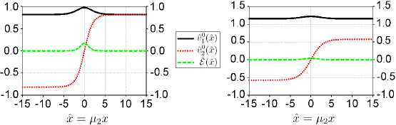
Figure 2: Plots of $\hat{v}_{1}^{0}(\hat{x})$, $\hat{v}_{2}^{0}(\hat{x})$ and the dimensionless energy density $\hat{\mathcal{E}}(\hat{x})$ for two different valid parameter sets of the $\mathrm{Z}_{2}$ invariant potential. The parameter sets used are $\{1,1,0.5\}$ (LHS) and $\{1.5,1,0.5\}$ (RHS), and the region of integration has $R=15$.

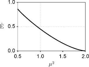
Figure 3: Numerical evaluation of the dependence of the dimensionless energy $\hat{\mathrm{E}}$ as a function of $\mu^{2}$, for the $\mathrm{Z}_{2}$ invariant potential. Here, we use the fiducial values $\lambda=1$ and $g=0.5$. Convexity of the potential and global minima conditions for these values require that $\mu^{2}\in(0.5,2.0)$.

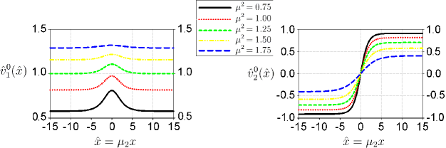
Figure 4: Plots comparing various $\hat{v}_{1}^{0}(\hat{x})$ (LHS plot) and $\hat{v}_{2}^{0}(\hat{x})$ (RHS plot) curves for the $\mathrm{Z}_{2}$ invariant potential by fixing $\lambda=1$ and $g=0.5$, and allowing $\mu^{2}$ to vary, and the region of integration $R=15$.

5.1.2 CP1 Domain Walls

From our analysis in Section 4.1, the 2HDM potential which is invariant under the CP1 symmetry can exhibit a disconnected vacuum manifold, the components of which are not linked by the gauge symmetries of the theory, provided both VEVs of the Higgs doublets $\phi_{1,2}$ and the relative phase between the doublets that create the neutral vacuum global minimum solution are non-zero, i.e. $v_{1,2}^{0}\neq 0$, $v_{2}^{+}=0$ and $\xi\neq 0$. This spontaneous violation of CP is only apparent within the CP1-invariant 2HDM when the determinant of the matrix $\rm N_{\mu\nu}$ vanishes, as shown in Section 4.1.1. However, as we have shown in Section 4.1, a neutral vacuum solution with a CP-conserving global minimum is also possible, where $\rm det[N_{\mu\nu}]\neq 0$, i.e. a global minimum with $v^{0}_{1,2}\neq 0$, $v_{2}^{+}=0$ and $\xi=0$. Therefore, during our numerical analysis we are careful to choose parameter sets that give global minimum neutral vacuum solutions with spontaneous CP violation.

Let us now investigate an one-dimensional, time-independent kink solution for the CP1 symmetry. In order to find such a solution, we will use an ansatz for the two Higgs doublets given by

$$\phi_{1}(x)\ =\ \frac{1}{\sqrt{2}}\left(\begin{array}[]{c}0\\ \vskip 6.0pt plus 2.0pt minus 2.0pt\cr v^{0}_{1}(x)\end{array}\right)\;,\quad\phi_{2}(x)\ =\ \frac{1}{\sqrt{2}}\left(\begin{array}[]{c}0\\ \vskip 6.0pt plus 2.0pt minus 2.0pt\cr v^{0}_{2}(x)e^{i\xi(x)}\end{array}\right)\;,$$ (5.11)

where the coordinate $x$ describes the spatial dimension perpendicular to the plane of the domain wall. The energy per unit area associated with the kink solution is again given by (5.2), where the energy density for the CP1-invariant 2HDM is given by

$$\mathcal{E}(x)\! = \!\frac{1}{2}\left(\frac{dv_{1}^{0}}{dx}\right)^{2}+\frac{1}{2}\left(\frac{dv_{2}^{0}}{dx}\right)^{2}+\frac{1}{2}v_{2}^{0}(x)^{2}\left(\frac{d\xi}{dx}\right)^{2}-\frac{1}{2}\mu_{1}^{2}v^{0}_{1}(x)^{2}-\frac{1}{2}\mu_{2}^{2}v^{0}_{2}(x)^{2}$$ (5.12)

$$+\frac{1}{4}\lambda_{1}v^{0}_{1}(x)^{4}+\frac{1}{4}\lambda_{2}v^{0}_{2}(x)^{4}+\frac{1}{4}\big{(}\lambda_{34}+\lambda_{5}\cos 2\xi(x)\big{)}v^{0}_{1}(x)^{2}v^{0}_{2}(x)^{2}$$

$$+\Big{(}-m_{12}^{2}+\frac{1}{2}\lambda_{6}v_{1}^{0}(x)^{2}+\frac{1}{2}\lambda_{7}v_{2}^{0}(x)^{2}\Big{)}v_{1}^{0}(x)v_{2}^{0}(x)\cos\xi(x)+\mathrm{V}_{0}\;.$$

By rescaling (5.2) to be dimensionless for the CP1 energy density, we again make use of the dimensionless quantities of (5.5). Performing these rescalings leaves the dimensionless CP1 energy density dependent on the following parameters:

$$\mu^{2}=\frac{\mu_{1}^{2}}{\mu_{2}^{2}}\;,\;\;m^{2}=\frac{m_{12}^{2}}{\mu_{2}^{2}}\;,\;\;\lambda=\frac{\lambda_{1}}{\lambda_{2}}\;,\;\;g_{34}=\frac{\lambda_{34}}{\lambda_{2}}\;,\;\;g_{k}=\frac{\lambda_{k}}{\lambda_{2}}\;\;\big{(}{\rm for}\;k=5,6,7\big{)}\;,\;\;\eta=\frac{\mu_{2}}{\sqrt{\lambda_{2}}}\;.$$ (5.13)

It is also useful to introduce the parameter $\bar{g}=g_{34}-g_{5}$. The parameter set for the CP1-invariant model then reduces and becomes $\{\mu^{2},m^{2},\lambda,g_{34},g_{5},g_{6},g_{7}\}$. Similarly, the vacuum manifold parameters $v_{1,2}^{0}$ and $\xi$ of (4.8a), (4.8b) and (4.8c), which are the boundary conditions on the fields $v_{1,2}^{0}(x)$ and $\xi(x)$, are rescaled, so as to give

$$\lim_{\hat{x}\to\pm\infty}\hat{v}^{0}_{1}(\hat{x})\ =\ \sqrt{\frac{2\left(g_{6}g_{7}-\bar{g}g_{5}\right)+2\left(2g_{5}-g_{7}^{2}\right)\mu^{2}+2\left(\bar{g}g_{7}-2g_{6}\right)m^{2}}{g_{5}\left(4\lambda-\bar{g}^{2}\right)-2\lambda g_{6}^{2}-2g_{7}^{2}+2\bar{g}g_{6}g_{7}}}\ ,$$ (5.14a)

$$\lim_{\hat{x}\to\pm\infty}\hat{v}^{0}_{2}(\hat{x})\ =\ \sqrt{\frac{2\left(2\lambda g_{5}-g_{6}^{2}\right)+2\left(g_{6}g_{7}-\bar{g}g_{5}\right)\mu^{2}+2\left(\bar{g}g_{6}-2\lambda g_{7}\right)m^{2}}{g_{5}\left(4\lambda-\bar{g}^{2}\right)-2\lambda g_{6}^{2}-2g_{7}^{2}+2\bar{g}g_{6}g_{7}}}\;,$$ (5.14b)

$$\lim_{\hat{x}\to\pm\infty}\xi(\hat{x})\ =\ \pm\mathrm{arccos}\left(\frac{2m^{2}-g_{6}(\hat{v}_{1}^{0})^{2}-g_{7}(\hat{v}_{2}^{0})^{2}}{2g_{5}\hat{v}_{1}^{0}\hat{v}_{2}^{0}}\right)\;.$$ (5.14c)

The equations of motion for the three rescaled fields $\hat{v}_{1,2}^{0}(\hat{x})$ and $\xi(\hat{x})$ are

$$\frac{d^{2}\hat{v}^{0}_{1}}{d\hat{x}^{2}}\ =\ \left[-\mu^{2}+\lambda(\hat{v}^{0}_{1})^{2}+\frac{1}{2}\left(g_{34}+g_{5}\cos 2\xi\right)(\hat{v}^{0}_{2})^{2}+\frac{3}{2}g_{6}\hat{v}^{0}_{1}\hat{v}^{0}_{2}\cos\xi\right]\,\hat{v}^{0}_{1}$$

$$\hskip 56.9055pt-\left[m^{2}-\frac{1}{2}g_{7}(\hat{v}^{0}_{2})^{2}\right]\hat{v}^{0}_{2}\cos\xi\,,$$ (5.15a)

$$\frac{d^{2}\hat{v}^{0}_{2}}{d\hat{x}^{2}}\ =\ \left[-1+\ (\hat{v}^{0}_{2})^{2}+\frac{1}{2}\left(g_{34}+g_{5}\cos 2\xi\right](\hat{v}^{0}_{1})^{2}+\frac{3}{2}g_{7}\hat{v}^{0}_{1}\hat{v}^{0}_{2}\cos\xi\right]\hat{v}^{0}_{2}$$

$$\hskip 56.9055pt-\ \left[m^{2}-\frac{1}{2}g_{6}(\hat{v}^{0}_{1})^{2}\right]\hat{v}^{0}_{1}\cos\xi\ +\ \left(\frac{d\xi}{d\hat{x}}\right)^{2}\hat{v}^{0}_{2}\;,$$ (5.15b)

$$(\hat{v}^{0}_{2})^{2}\frac{d^{2}\xi}{d\hat{x}^{2}}\ +\ 2\hat{v}^{0}_{2}\left(\frac{d\xi}{d\hat{x}}\right)\left(\frac{d\hat{v}^{0}_{2}}{d\hat{x}}\right)\ =$$

$$\hskip 56.9055pt-\hat{v}^{0}_{1}\hat{v}^{0}_{2}\sin\xi\left[g_{5}\hat{v}^{0}_{1}\hat{v}^{0}_{2}\cos\xi-m^{2}+\frac{1}{2}g_{6}(\hat{v}^{0}_{1})^{2}+\frac{1}{2}g_{7}(\hat{v}^{0}_{2})^{2}\right].$$ (5.15c)

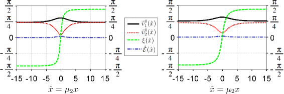
Figure 5: Plots of $\hat{v}_{1}^{0}(\hat{x})$, $\hat{v}_{2}^{0}(\hat{x})$, $\xi(\hat{x})$ and the dimensionless energy density $\hat{\mathcal{E}}(\hat{x})$ for two different valid parameter sets of the CP1-invariant potential. The parameter sets used are $\{1,0.1,1,2.5,1,0,0\}$ (LHS) and $\{1,0.1,1,2.5,1,-0.15,0.15\}$ (RHS). The region of integration has $R=15$.

As with the $\rm Z_{2}$ domain wall study, no analytical solution is found to these equations of motion and we therefore proceed by gradient flow techniques. Due to the number of individual parameters one may tune within the confines of the CP1 convexity and minima conditions, relationships between the parameters are in general complicated and so we end our CP1 domain wall study by presenting two typical solutions in Figure 5. However, we do note two cases determined by specific choices of the parameter set. For the case $\displaystyle\lim_{\hat{x}\to\pm\infty}\xi(\hat{x})=\frac{\pi}{2}$, which is guaranteed if $g_{6}(\hat{v}_{1}^{0})^{2}+g_{7}(\hat{v}_{2}^{0})^{2}=2m^{2}$, the CP1 symmetry domain wall reverts back to a $\rm Z_{2}$ style domain wall by use of the reparameterization $\phi_{2}\to i\phi_{2}$, as discussed in Section 4.1.2. An explicit example can be seen for the $\rm Z_{2}$ symmetry potential parameters constraints, $m_{12}^{2}=\lambda_{6}=\lambda_{7}=0$. Also, the dimensionless energy $\rm\hat{E}$ can be made vanishingly small for certain valid choices of the parameter set that leave the limit of (5.14c) still finite but $\ll 1$. This is consistent with the case $\displaystyle\lim_{\hat{x}\to\pm\infty}\xi(\hat{x})=0$ in which spontaneous CP violation ceases and subsequently there is no domain wall solution, as discussed in Section 4.1.2.

5.1.3 CP2 Domain Walls

From our analysis in Section 4.2, the 2HDM potential which is invariant under the CP2 symmetry can exhibit a disconnected vacuum manifold, the components of which are not linked by the gauge symmetries of the theory, provided both VEVs of the Higgs doublets $\phi_{1,2}$ that create the neutral vacuum global minimum solution are non-zero, i.e. $v_{1,2}^{0}\neq 0$, $v_{2}^{+}=0$. This scenario is only apparent within the CP2-invariant 2HDM when the determinant of the matrix $\rm N_{\mu\nu}$ vanishes, as shown in Section 4.2.1

We now investigate an one-dimensional, time-independent kink solution for the CP2 symmetry. In order to find such a solution, we will use an ansatz for the two Higgs doublets given by (5.11). The energy per unit area associated with the kink solution is again given by (5.2). The energy density for the CP2-invariant 2HDM is given by

$$\mathcal{E}(x)\! = \!\frac{1}{2}\left(\frac{dv_{1}^{0}}{dx}\right)^{2}+\frac{1}{2}\left(\frac{dv_{2}^{0}}{dx}\right)^{2}+\frac{1}{2}v_{2}^{0}(x)^{2}\left(\frac{d\xi}{dx}\right)^{2}-\frac{1}{2}\mu_{1}^{2}\big{(}v^{0}_{1}(x)^{2}+v^{0}_{2}(x)^{2}\big{)}$$ (5.16)

$$+\ \frac{1}{4}\lambda_{1}\big{(}v^{0}_{1}(x)^{4}+v^{0}_{2}(x)^{4}\big{)}+\frac{1}{4}\big{(}\lambda_{34}+R_{5}\cos 2\xi(x)-I_{5}\sin 2\xi(x)\big{)}v^{0}_{1}(x)^{2}v^{0}_{2}(x)^{2}$$

$$+\ \frac{1}{2}v_{1}^{0}(x)v_{2}^{0}(x)\big{(}v_{1}^{0}(x)^{2}-v_{2}^{0}(x)^{2}\big{)}\big{(}R_{6}\cos\xi(x)-I_{6}\sin\xi(x)\big{)}\ +\ \mathrm{V}_{0}\;.$$

Again, it is useful to rescale (5.2) to be dimensionless for the CP2 energy density, and so we introduce

$$\hat{x}\ =\ \mu_{1}x\;,\qquad\hat{v}_{1,2}^{0}(x)\ =\ \frac{v^{0}_{1,2}(x)}{\eta}\;,\qquad\hat{\mathrm{E}}\ =\ \frac{\lambda_{1}\mathrm{E}}{\mu_{1}^{3}}\;.$$ (5.17)

Performing these rescalings leaves the dimensionless CP2 energy density $\hat{\cal E}$ dependent on the following parameters:

$$g_{k}\ =\ \frac{R_{k}}{\lambda_{1}}\ \ \big{(}{\rm for}\;k=3,4,5,6\big{)}\;,\quad h_{k}\ =\ \frac{I_{k}}{\lambda_{1}}\ \ \big{(}{\rm for}\;k=5,6\big{)}\;,\quad\eta\ =\ \frac{\mu_{1}}{\sqrt{\lambda_{1}}}\;.$$ (5.18)

Therefore, the parameter set for the CP2-invariant model becomes $\{g_{3},g_{4},g_{5},g_{6},h_{5},h_{6}\}$. Also, the vacuum manifold parameters $v_{1,2}^{0}$ and $\xi$ of (4.20a), (4.20b) and (4.20c), which are the boundary conditions on the fields $v_{1,2}^{0}(x)$ and $\xi(x)$, are rescaled as follows:

$$\hat{v}^{0}_{1}(\hat{x})\ \to\ \left\{\begin{array}[]{cl}\displaystyle\sqrt{\left(\frac{2}{2+g_{3}-\hat{\zeta}}\right)\left(1-\frac{1}{\hat{\mathrm{B}}}\,\frac{2h_{5}g_{6}-2h_{6}(g_{4}+g_{5}+\hat{\zeta})}{4h_{6}g_{6}-h_{5}(2-g_{3}+\hat{\zeta})}\right)},\ \mbox{as $\hat{x}\to-\infty$}\vskip 12.0pt plus 4.0pt minus 4.0pt\\ \displaystyle\sqrt{\left(\frac{2}{2+g_{3}-\hat{\zeta}}\right)\left(1+\frac{1}{\hat{\mathrm{B}}}\,\frac{2h_{5}g_{6}-2h_{6}(g_{4}+g_{5}+\hat{\zeta})}{4h_{6}g_{6}-h_{5}(2-g_{3}+\hat{\zeta})}\right)},\ \mbox{as $\hat{x}\to+\infty$}\end{array}\right.\;,$$ (5.19c)

$$\hat{v}^{0}_{2}(\hat{x})\ \to\ \left\{\begin{array}[]{cl}\displaystyle-\sqrt{\left(\frac{2}{2+g_{3}-\hat{\zeta}}\right)\left(1+\frac{1}{\hat{\mathrm{B}}}\,\frac{2h_{5}g_{6}-2h_{6}(g_{4}+g_{5}+\hat{\zeta})}{4h_{6}g_{6}-h_{5}(2-g_{3}+\hat{\zeta})}\right)},\ \mbox{as $\hat{x}\to-\infty$}\vskip 12.0pt plus 4.0pt minus 4.0pt\\ \displaystyle\sqrt{\left(\frac{2}{2+g_{3}-\hat{\zeta}}\right)\left(1-\frac{1}{\hat{\mathrm{B}}}\,\frac{2h_{5}g_{6}-2h_{6}(g_{4}+g_{5}+\hat{\zeta})}{4h_{6}g_{6}-h_{5}(2-g_{3}+\hat{\zeta})}\right)},\ \mbox{as $\hat{x}\to+\infty$}\end{array}\right.\;,$$ (5.19f)

$$\lim_{\hat{x}\to\pm\infty}\xi(\hat{x})\ =\ \mathrm{arctan}\left(\frac{(g_{4}+g_{5}+\hat{\zeta})h_{6}-h_{5}g_{6}}{h_{5}h_{6}-(g_{4}-g_{5}+\hat{\zeta})g_{6}}\right)\;,$$ (5.19g)

where the parameter $\hat{\mathrm{B}}$ is defined as

$$\hat{\mathrm{B}}=\ \sqrt{\left(\frac{h_{5}g_{6}-h_{6}(g_{4}+g_{5}+\hat{\zeta})}{g_{6}(g_{4}-g_{5}+\hat{\zeta})-h_{5}h_{6}}\right)^{2}+\ \left(\frac{2h_{5}g_{6}-2h_{6}(g_{4}+g_{5}+\hat{\zeta})}{4h_{6}g_{6}-h_{5}(2-g_{3}+\hat{\zeta})}\right)^{2}+\ 1}\ .$$ (5.20)

These boundary conditions depend on the non-trivial Lagrange multiplier implemented to produce the neutral vacuum solution. This Lagrange multiplier satisfies the cubic equation:

$$\hat{\zeta}^{3}+\big{(}2-g_{3}+2g_{4}\big{)}\hat{\zeta}^{2}+\big{(}2g_{4}(2-g_{3})+g_{4}^{2}-g_{5}^{2}-h_{5}^{2}-4g_{6}^{2}-4h_{6}^{2}\big{)}\hat{\zeta}$$

$$+(2-g_{3})(g_{4}^{2}-g_{5}^{2}-h_{5}^{2})-4(g_{6}^{2}+h_{6}^{2})(g_{4}-g_{5})+8h_{6}(h_{5}g_{6}-g_{5}h_{6})\ =\ 0\;.$$ (5.21)

In order to find a valid parameter set, we start by choosing parameter values that satisfy the CP2 convexity conditions (shown in Table 9) and then solve (5.21) to find the three possible values of $\hat{\zeta}$. We then find the rescaled vacuum manifold parameters which correspond to each $\hat{\zeta}$ solution, and determine if these solutions correspond to local minima, i.e. we require that the CP2 Hessian matrix ${\rm H}$ in (4.22a)–(4.22f) be positive definite. If they do indeed relate to minima, we calculate the value of the potential at these extremal points to determine which $\hat{\zeta}$ solution generates the global minimum.

The equations of motion for the three rescaled fields $\hat{v}_{1,2}^{0}(\hat{x})$ and $\xi(\hat{x})$ are:

$$\frac{d^{2}\hat{v}^{0}_{1}}{d\hat{x}^{2}}\ =\ \hat{v}^{0}_{1}\left[-1+(\hat{v}^{0}_{1})^{2}+\frac{1}{2}\left(g_{34}+g_{5}\cos 2\xi-h_{5}\sin 2\xi\right)(\hat{v}^{0}_{2})^{2}\right]$$

$$\hskip 56.9055pt+\ \frac{1}{2}\hat{v}^{0}_{2}\left(3(\hat{v}^{0}_{1})^{2}\ -\ (\hat{v}^{0}_{2})^{2}\right)\left(g_{6}\cos\xi-h_{6}\sin\xi\right)\;,$$ (5.22a)

$$\frac{d^{2}\hat{v}^{0}_{2}}{d\hat{x}^{2}}\ =\ \hat{v}^{0}_{2}\left[-1+(\hat{v}^{0}_{2})^{2}+\frac{1}{2}\left(g_{34}+g_{5}\cos 2\xi-h_{5}\sin 2\xi\right)(\hat{v}^{0}_{1})^{2}+\left(\frac{d\xi}{d\hat{x}}\right)^{2}\right]$$

$$\hskip 56.9055pt+\ \frac{1}{2}\hat{v}^{0}_{1}\left((\hat{v}^{0}_{1})^{2}-3(\hat{v}^{0}_{2})^{2}\right)\left(g_{6}\cos\xi-h_{6}\sin\xi\right)\;,$$ (5.22b)

$$(\hat{v}^{0}_{2})^{2}\frac{d^{2}\xi}{d\hat{x}^{2}}\ +\ 2\hat{v}_{2}^{0}\left(\frac{d\hat{v}^{0}_{2}}{d\hat{x}}\right)\left(\frac{d\xi}{d\hat{x}}\right)\ =\ -\frac{1}{2}\hat{v}^{0}_{1}\hat{v}_{2}^{0}\left[\hat{v}^{0}_{1}\hat{v}^{0}_{2}\left(g_{5}\sin 2\xi+h_{5}\cos 2\xi\right)\right.$$

$$\hskip 56.9055pt\left.+\!\left((\hat{v}^{0}_{1})^{2}\!-\!(\hat{v}^{0}_{2})^{2}\right)\left(g_{6}\sin\xi\!+\!h_{6}\cos\xi\right)\right]\;.$$ (5.22c)

We can obtain numerical solutions to these equations of motion, by making use of gradient flow techniques. Since there is a large number of individual parameters that could vary within the confines of the CP2 convexity and minima conditions, relationships between the parameters are, in general, complicated. Instead, we present a typical example of CP2 domain walls, as shown in Figure 6. As with the previous two case, we observe that the dimensionless energy $\rm\hat{E}$ can be made vanishingly small for certain valid choices of the parameter set, such as allowing $g_{5,6}$ and $h_{5,6}$ to tend to zero.

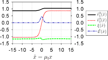
Figure 6: Numerical estimates of $\hat{v}_{1}^{0}(\hat{x})$, $\hat{v}_{2}^{0}(\hat{x})$, $\xi(\hat{x})$ and the dimensionless energy density $\hat{\mathcal{E}}(\hat{x})$, for a valid parameter set of the CP2-invariant potential. The input parameter set is $\{0.125,0.375,0.125,0.125,-0.25,-0.25\}$. The region of integration has $R=15$.

5.2 Vortices

We now turn our attention to other topological defects which may form in the 2HDM, such as vortices. Whilst vortex solutions have been discussed in the 2HDM [70], these vortices were generated by the SM gauge group, whereas the vortices we discuss here are generated solely by the spontaneous breaking of the ${\rm U(1)}_{\rm PQ}$ and CP3 accidental symmetries which the 2HDM can exhibit for specific constraints on the parameters of the potential.

Vortices are often regarded as the most favourable topological defect, since their energy density does not grow relative to the background and so for sufficiently small initial energy densities, vortices behave benignly and can comply with current cosmological observations. Due to the axially symmetric, one-dimensional and typically high mass density characteristics of a cosmic string, strings can act as a gravitational lens [71, 72] and searches are already under way to detect possible vortices which may be within the current horizon, e.g. using precision cosmic microwave background data from experiments such as WMAP [73, 74].

As with our domain wall study, we do not study the cosmological implications of the 2HDM’s vortices, which we reserve for a future study, but focus on presenting an overview of typical solutions and determining whether or not the energy per unit length of the vortex can be made to be vanishingly small for specific and valid choices of the model parameters.

5.2.1 $\mathrm{U(1)}_{\mathrm{PQ}}$ Vortices

From our analysis in Section 3.2, the 2HDM potential which is invariant under the global Peccei-Quinn U(1) symmetry can exhibit a non-simply connected vacuum manifold provided both VEVs of the Higgs doublets $\phi_{1,2}$ that create the neutral vacuum global minimum solution are non-zero, i.e. $v_{1,2}^{0}\neq 0$ and $v_{2}^{+}=0$. This scenario is only apparent within the $\mathrm{U(1)}_{\mathrm{PQ}}$ invariant 2HDM when the determinant of the matrix $\rm N_{\mu\nu}$ vanishes, as shown in Section 3.2.1.

In order to find a two-dimensional time-independent vortex solution for the $\rm U(1)_{PQ}$ symmetry, we use the ansatz for the two Higgs doublets:

$$\phi_{1}(r)\ =\ \frac{1}{\sqrt{2}}\left(\begin{array}[]{c}0\\ \vskip 6.0pt plus 2.0pt minus 2.0pt\cr v^{0}_{1}(r)\end{array}\right)\;,\qquad\phi_{2}(r,\chi)\ =\ \frac{1}{\sqrt{2}}\left(\begin{array}[]{c}0\\ \vskip 6.0pt plus 2.0pt minus 2.0pt\cr v^{0}_{2}(r)e^{in\chi}\end{array}\right)\;,$$ (5.23)

where the coordinate $r$ describes the space radially outward from the core of the vortex, and $\chi$ is an azimuthal angle which accounts for the winding of the vortex, with winding number $n$. Using this ansatz, the energy per unit length of the system is then:

$$\mathrm{E}\ =\ 2\pi\int_{0}^{\infty}\!\!\!\!\!rdr\;\;\mathcal{E}\!\left(\phi_{1},\phi_{2}\right)\;,$$ (5.24)

where the energy density for the $\mathrm{U(1)}_{\mathrm{PQ}}$ invariant 2HDM is given by

$$\mathcal{E}\!\left(r\right) = \frac{1}{2}\left(\frac{dv^{0}_{1}}{dr}\right)^{2}+\frac{1}{2}\left(\frac{dv^{0}_{2}}{dr}\right)^{2}+\frac{n^{2}}{2r^{2}}v^{0}_{2}(r)^{2}-\frac{1}{2}\mu_{1}^{2}v^{0}_{1}(r)^{2}-\frac{1}{2}\mu_{2}^{2}v^{0}_{2}(r)^{2}$$ (5.25)

$$+\frac{1}{4}\lambda_{1}v^{0}_{1}(r)^{4}+\frac{1}{4}\lambda_{2}v^{0}_{2}(r)^{4}+\frac{1}{4}\lambda_{34}v^{0}_{1}(r)^{2}v^{0}_{2}(r)^{2}+\mathrm{V}_{0}\;.$$

For this type of energy density, the integral of (5.24) is logarithmically divergent in $r$, so we truncate the region of integration from $[0,\infty)$ to $[0,R]$, where $R$ is a cut off radius [41]. To once again simplify our study, we rescale the energy per unit length of the vortex in (5.24) to be dimensionless by introducing the dimensionless quantities

$$\hat{r}\ =\ \mu_{2}r\;,\quad\hat{v}_{1,2}^{0}(r)\ =\ \frac{v_{1,2}^{0}(r)}{\eta}\;,\quad\hat{\mathrm{E}}\ =\ \frac{\mathrm{E}}{2\pi\eta^{2}}\;.$$ (5.26)

With the help of these rescalings, the dimensionless $\rm U(1)_{PQ}$ energy density derived from (5.24) depends now on the following parameters:

$$\mu^{2}\ =\ \frac{\mu_{1}^{2}}{\mu_{2}^{2}}\;,\quad\lambda\ =\ \frac{\lambda_{1}}{\lambda_{2}}\;,\quad g\ =\ \frac{\lambda_{34}}{2\lambda_{2}}\;,\quad\eta\ =\ \frac{\mu_{2}}{\sqrt{\lambda_{2}}}\;.$$ (5.27)

Having rescaled the vacuum manifold parameters $\hat{v}_{1,2}^{0}(\hat{r})$, we require that these approach their corresponding VEVs given in (3.26a) and (3.26b), as $r\to\infty$. To be precise, we impose the boundary conditions:

$$\left.\frac{d\hat{v}^{0}_{1}}{d\hat{r}}\right|_{\hat{r}=0}\ =\ 0\;, \qquad\lim_{\hat{r}\to\infty}\hat{v}^{0}_{1}(\hat{r})\ =\ \sqrt{\frac{\mu^{2}-g}{\lambda-g^{2}}}\ ,$$ (5.28a)

$$\lim_{\hat{r}\to 0}\hat{v}^{0}_{2}(\hat{r})\ =\ 0\;, \qquad\lim_{\hat{r}\to\infty}\hat{v}^{0}_{2}(\hat{r})\ =\ \sqrt{\frac{\lambda-\mu^{2}g}{\lambda-g^{2}}}\ .$$ (5.28b)

These conditions force $\hat{v}^{0}_{2}(\hat{r})$ to be regular for all values of $\hat{r}$ and require $\hat{v}^{0}_{1}(\hat{r})$ to be continuous and radially symmetric. The equations of motion for the two rescaled fields $\hat{v}^{0}_{1,2}(\hat{r})$ are found to be

$$\frac{d^{2}\hat{v}^{0}_{1}}{d\hat{r}^{2}}\ =\ \hat{v}^{0}_{1}\;\big{(}-\mu^{2}+\lambda(\hat{v}^{0}_{1})^{2}+g(\hat{v}^{0}_{2})^{2}\big{)}\ ,$$ (5.29a)

$$\frac{d^{2}\hat{v}^{0}_{2}}{d\hat{r}^{2}}\ +\ \frac{1}{\hat{r}}\frac{d\hat{v}^{0}_{2}}{d\hat{r}}\ =\ \hat{v}^{0}_{2}\;\Big{(}-1+\frac{n^{2}}{\hat{r}^{2}}+(\hat{v}^{0}_{2})^{2}+g(\hat{v}^{0}_{1})^{2}\Big{)}\;.$$ (5.29b)

As is typical of vortex studies, no analytical solutions to the equations of motion are found and so we make use of gradient flow numerical techniques.

For our numerical analysis, we choose a particular parameter set $\{\mu^{2},\lambda,g,n\}$ that satisfies the constraints for a bounded-from-below global minimum, which are of exactly the same form as for the $\rm Z_{2}$ symmetry in (5.9). In order to satisfy that $(v^{0}_{1})^{2}+(v^{0}_{2})^{2}=v^{2}_{\rm SM}$, we require that the VEV scale factor $\eta$ have the value given by (5.10). We note that a value of $\eta$ can always be found that ensures condition (5.10) is met for any parameter set $\{\mu^{2},\lambda,g,n\}$, provided that the members of the parameter set remain non-zero and finite, and satisfy the conditions in (5.9).

We conclude our $\mathrm{U(1)}_{\mathrm{PQ}}$ vortex study by presenting two typical solutions in Figure 7. We show the general form of the dimensionless energy $\rm\hat{E}$ in Figure 8, as a function of $\mu^{2}$, noting that the dimensionless energy tends to zero as $\mu^{2}$ approaches its upper limit, i.e. $\mu^{2}\to\frac{\lambda}{g}$. We also directly compare several different solutions in Figures 9 and 10 by varying $\mu^{2}$ and the winding number $n$ respectively. From Figures 9 and 10 in particular, we see that as $\mu^{2}$ increases, the width of the vortex core increases and similarly, as the winding number increases, so does the width of the vortex core.

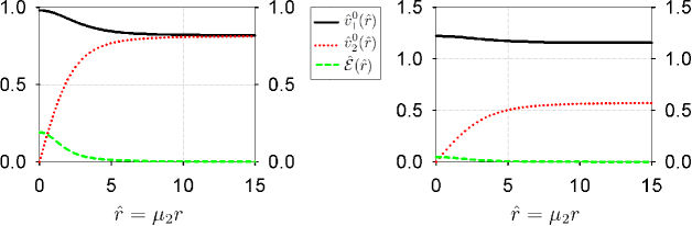
Figure 7: Plots of $\hat{v}_{1}^{0}(\hat{r})$, $\hat{v}_{2}^{0}(\hat{r})$ and the dimensionless energy density $\hat{\mathcal{E}}(\hat{r})$ for two different valid parameter sets of the $\mathrm{U(1)}_{\mathrm{PQ}}$ invariant potential. The parameter sets used are $\{1,1,0.5,1\}$ (LHS) and $\{1.5,1,0.5,1\}$ (RHS). The cut off radius used for both plots is $R=15$.

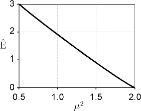
Figure 8: Numerical evaluation of the dimensionless energy $\hat{\mathrm{E}}$, as a function of $\mu^{2}$ for the $\mathrm{U(1)}_{\mathrm{PQ}}$ invariant potential. Here, we use the fiducial values $\lambda=1$, $g=0.5$ and $n=1$. Convexity of the potential and global minima conditions for these values require that $\mu^{2}\in(0.5,2.0)$.

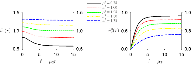
Figure 9: Plots comparing various $\hat{v}_{1}^{0}(\hat{r})$ (LHS plot) and $\hat{v}_{2}^{0}(\hat{r})$ (RHS plot) curves for the $\mathrm{U(1)}_{\mathrm{PQ}}$ invariant potential. Here, we fix $\lambda=1$, $g=0.5$ and $n=1$, and allow $\mu^{2}$ to vary. The cut off radius used for both plots is $R=15$.

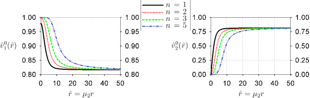
Figure 10: Plots comparing various $\hat{v}_{1}^{0}(\hat{r})$ (LHS plot) and $\hat{v}_{2}^{0}(\hat{r})$ (RHS plot) curves for the $\mathrm{U(1)}_{\mathrm{PQ}}$ invariant potential for various winding numbers $n$. Here, we fix $\lambda=1$, $g=0.5$ and $\mu^{2}=1$, and allow $n$ to vary. The cut off radius used for both plots is $R=50$

5.2.2 CP3 Vortices

As discussed in Section 4.3, the CP3-symmetric 2HDM potential can exhibit a non-simply connected vacuum manifold, provided a neutral vacuum global minimum solution exists where the sum of the squares of the two VEVs of the doublets $\phi_{1,2}$ is non-zero. Such a scenario can be realized within the CP3-invariant 2HDM, if the matrix $\rm N_{\mu\nu}$ happens to be singular. However, as shown in Section 4.3.1, there are two possible neutral vacuum solutions that could form the global minimum solution, depending on the relative magnitudes of the quantities $2\lambda_{1}$ and $\lambda_{34}$. If $2\lambda_{1}>\lambda_{34}$, we find that any possible vortex solution can be removed by gauge transformations, whereas for cases with $\lambda_{34}>2\lambda_{1}$, no such gauge transformations are possible, allowing a vortex solution. Hence, we study cases of the latter type to ensure vortex formation in the CP3-invariant potential.

In order to obtain a time-independent vortex solution for the CP3 symmetry, the following ansatz for the two Higgs doublets is used:

$$\phi_{1}(r,\chi)\ =\ \frac{1}{\sqrt{2}}\left(\begin{array}[]{c}0\\ \vskip 6.0pt plus 2.0pt minus 2.0pt\cr v(r)\cos(n\chi)\end{array}\right)\;,\qquad\phi_{2}(r,\chi)\ =\ \frac{1}{\sqrt{2}}\left(\begin{array}[]{c}0\\ \vskip 6.0pt plus 2.0pt minus 2.0pt\cr-v(r)\sin(n\chi)\end{array}\right)\;,$$ (5.30)

where the coordinate $r$ describes the space radially outward from the core of the vortex, and $\chi$ is an azimuthal angle which accounts for the winding of the vortex, with winding number $n$. Using this ansatz, the energy per unit length of the system is given by (5.24) where the energy density for the CP3-invariant 2HDM is given by

$$\mathcal{E}\!\left(r\right)\ =\ \frac{1}{2}\left(\frac{dv}{dr}\right)^{2}+\frac{n^{2}}{2r^{2}}v(r)^{2}-\frac{1}{2}\mu_{1}^{2}v(r)^{2}+\frac{1}{4}\lambda_{1}v(r)^{4}\ +\ \mathrm{V}_{0}\;.$$ (5.31)

As before, (5.24) is logarithmically divergent for the CP3 energy density and so we truncate (5.24) to a cut off radius $r=R$. Our study can be simplified, if we rescale the energy per unit length of the vortex in (5.24) to be dimensionless and introduce the dimensionless quantities

$$\hat{r}\ =\ \mu_{1}r\;,\qquad\hat{v}(r)\ =\ \frac{v(r)}{\eta}\;,\qquad\hat{\mathrm{E}}\ =\ \frac{\mathrm{E}}{2\pi\eta^{2}}\;,$$ (5.32)

Figure 11: Plots of $\hat{v}(\hat{r})$ (LHS plot) and the dimensionless energy density $\hat{\mathcal{E}}(\hat{r})$ (RHS plot) for the CP3-invariant potential. The winding number $n$ is varied from 1 to 5 and the cut off radius for both plots is $R=30$.

with $\eta=\frac{\mu_{1}}{\sqrt{\lambda_{1}}}$. We then require that $(v^{0}_{1})^{2}+(v^{0}_{2})^{2}=v^{2}_{\rm SM}$ and also $\eta=v_{\rm SM}$. Under the above parameter re-definitions and provided the winding number $n$ is non-zero, the boundary conditions on the vacuum field $\hat{v}(\hat{r})$, which follows from (4.29a), become

$$\lim_{\hat{r}\to 0}\hat{v}(\hat{r})\ =\ 0\;,\qquad\lim_{\hat{r}\to\infty}\hat{v}(\hat{r})\ =\ 1\;.$$ (5.33)

These conditions force $\hat{v}(\hat{r})$ to be regular for all values of $\hat{r}$ and ensure that the dimensionful field $v(r)$ approaches its VEV in the limit $r\to\infty$. The equation of motion for the rescaled field $\hat{v}(\hat{r})$ is

$$\frac{d^{2}\hat{v}}{d\hat{r}^{2}}\ +\ \frac{1}{\hat{r}}\frac{d\hat{v}}{d\hat{r}}\ =\ \hat{v}\;\Big{(}-1+\frac{n^{2}}{\hat{r}^{2}}+\hat{v}^{2}\Big{)}\;.$$ (5.34)

The above differential equation is solved numerically, by means of gradient flow methods. Our numerical analysis only depends on the choice of the single parameter $n$, i.e. the winding number. Figure 11 presents the dependence of $\hat{v}$ and the corresponding energy density $\hat{\cal E}$, as a function of $\hat{r}$, for various values of $n$. We observe that as the value of $n$ increases, the width of the vortex core increases and the energy density radially spreads out, giving the characteristic volcano shape.

5.3 Global Monopoles

We complete our study of the topological defects that may form in the 2HDM due to the spontaneous breaking of the 6 accidental symmetries with the global monopole. This topological solution arises from the symmetry breaking of the $\rm SO(3)_{HF}$ symmetry to its subgroup $\rm SO(2)_{HF}$. In spite of being intrinsically unstable, global monopoles may have important cosmological implications, as they can provide a mechanism for structure formation within the Universe [50].

As with our previous topological defect studies, we do not analyse the cosmological implications of the 2HDM’s global monopole, but focus on presenting an overview of possible solutions.

5.3.1 SO$(3)_{\mathrm{HF}}$ Global Monopoles

Our analysis in Section 3.3 has shown that a $\rm SO(3)_{HF}$-invariant 2HDM potential can exhibit a vacuum manifold containing non-contractible 2-spheres, provided a neutral vacuum solution for a global minimum exists, such that $(v^{0}_{1})^{2}+(v^{0}_{2})^{2}=v^{2}_{\rm SM}$. This scenario is only possible in the $\rm SO(3)_{HF}$-invariant 2HDM, for a singular matrix $\rm N_{\mu\nu}$ [cf. Section 3.3.1].

We may seek a time-independent spherically symmetric global monopole solution for the $\rm SO(3)_{HF}$ symmetry, by making use of the following ansatz for the two Higgs doublets:

$$\phi_{1}(r,\chi)\ =\ \frac{1}{\sqrt{2}}\left(\begin{array}[]{c}0\\ \vskip 6.0pt plus 2.0pt minus 2.0pt\cr v(r)\sin\chi\end{array}\right)\;,\qquad\phi_{2}(r,\chi,\psi)\ =\ \frac{1}{\sqrt{2}}\left(\begin{array}[]{c}0\\ \vskip 6.0pt plus 2.0pt minus 2.0pt\cr v(r)e^{i\psi}\cos\chi\end{array}\right)\;,$$ (5.35)

where the coordinate $r$ describes the space radially outward from axis of symmetry of the monopole, $\chi$ is an azimuthal angle and $\psi$ is a polar angle. Using this ansatz, the energy per monopole is

$$\mathrm{E}\ =\ 4\pi\int_{0}^{\infty}\!\!\!r^{2}dr\;\;\mathcal{E}\!\left(\phi_{1},\phi_{2}\right)\;,$$ (5.36)

where the energy density for the $\rm SO(3)_{HF}$ invariant 2HDM is given by

$$\mathcal{E}\!\left(r\right)\ =\ \frac{1}{2}\left(\frac{dv}{dr}\right)^{2}+\frac{1}{r^{2}}v(r)^{2}-\frac{1}{2}\mu_{1}^{2}v(r)^{2}+\frac{1}{4}\lambda_{1}v(r)^{4}\ +\ \mathrm{V}_{0}\;,$$ (5.37)

For this type of energy density, the integral of (5.36) is linearly divergent in $r$, so we truncate the region of integration from $[0,\infty)$ to $[0,R]$, where $R$ is a cut off radius [41]. Our study gets considerably simplified, if we rescale (5.36) to become dimensionless and introduce the dimensionless quantities

$$\hat{r}\ =\ \mu_{1}r\;,\qquad\hat{v}(r)\ =\ \frac{v(r)}{\eta}\;,\qquad\hat{\mathrm{E}}\ =\ \frac{\lambda_{1}\mathrm{E}}{4\pi\mu_{1}}\;.$$ (5.38)

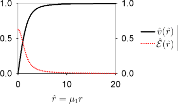
Figure 12: Plots of $\hat{v}(\hat{r})$ and the dimensionless energy density $\hat{\mathcal{E}}(\hat{r})$ for the $\rm SO(3)_{HF}$ invariant potential. The cut off radius for this plot is $R=20$.

We then define $\eta=\frac{\mu_{1}}{\sqrt{\lambda_{1}}}$ and require that $\eta=v_{\rm SM}$. Under these rescalings, the boundary conditions on the vacuum field $\hat{v}(\hat{r})$, which follow from (3.37), become

$$\lim_{\hat{r}\to 0}\hat{v}(\hat{r})\ =\ 0\;,\qquad\lim_{\hat{r}\to\infty}\hat{v}(\hat{r})\ =\ 1\;.$$ (5.39)

These conditions force $\hat{v}(\hat{r})$ to be regular for all values of $\hat{r}$ and ensures the dimensionful field $v(r)$ approaches its VEV in the limit $r\to\infty$. The equation of motion for the rescaled field $\hat{v}(\hat{r})$ is

$$\frac{d^{2}\hat{v}}{d\hat{r}^{2}}\ +\ \frac{2}{\hat{r}}\frac{d\hat{v}}{d\hat{r}}\ =\ \hat{v}\;\Big{(}-1+\frac{2}{\hat{r}^{2}}+\hat{v}^{2}\Big{)}\;.$$ (5.40)

As with the majority of monopole studies, we rely on gradient flow techniques to numerically solve the above differential equation. In Figure 12, we present the single solution for an $\rm SO(3)_{HF}$ global monopole, by displaying the $\hat{r}$-dependence of the vacuum field $\hat{v}(\hat{r})$ and its respective dimensionless energy density $\hat{\cal E}$.

6 The U(1)_Y-Violating 2HDM

In this section we discuss the application of our Majorana scalar-field formalism to 2HDM potentials which are not restricted by the ${\rm U(1)_{Y}}$ hypercharge group. Even though such potentials may not be viable within the context of the SM, they may still be realized in models describing cosmological inflation [44, 45]. Furthermore, we classify all possible 15 symmetries that may occur in a general $\rm U(1)_{Y}$-violating 2HDM potential, within the 6-dimensional bilinear field space.

If conservation under some ${\rm U(1)_{Y}}$ hypercharge group is lifted from the theory, then additional SU(2) gauge-invariant bilinears can, in principle, be present in the 2HDM potential, such as $\phi_{1}^{\mathrm{T}}i\sigma^{2}\phi_{2}$ and its Hermitian conjugate, $-\phi_{2}^{\dagger}i\sigma^{2}\phi_{1}^{*}$. Counting the number of real independent parameters, the resulting potential would have 6 bilinear mass terms and 20 quartic terms. Its explicit analytic form is given by

$$\mathrm{V}\!\!\!\!\!\!\!\!\! =-\mu_{1}^{2}(\phi_{1}^{\dagger}\phi_{1})-\mu_{2}^{2}(\phi_{2}^{\dagger}\phi_{2})-m_{12}^{2}(\phi_{1}^{\dagger}\phi_{2})-m_{12}^{*2}(\phi_{2}^{\dagger}\phi_{1})-m_{34}^{2}(\phi_{1}^{\mathrm{T}}i\sigma^{2}\phi_{2})+m_{34}^{*2}(\phi_{2}^{\dagger}i\sigma^{2}\phi_{1}^{*})$$ (6.1)

$$+\lambda_{1}(\phi_{1}^{\dagger}\phi_{1})^{2}+\lambda_{2}(\phi_{2}^{\dagger}\phi_{2})^{2}+\lambda_{3}(\phi_{1}^{\dagger}\phi_{1})(\phi_{2}^{\dagger}\phi_{2})+\lambda_{4}(\phi_{1}^{\dagger}\phi_{2})(\phi_{2}^{\dagger}\phi_{1})+\frac{\lambda_{5}}{2}(\phi_{1}^{\dagger}\phi_{2})^{2}+\frac{\lambda_{5}^{*}}{2}(\phi_{2}^{\dagger}\phi_{1})^{2}$$

$$+\lambda_{6}(\phi_{1}^{\dagger}\phi_{1})(\phi_{1}^{\dagger}\phi_{2})+\lambda_{6}^{*}(\phi_{1}^{\dagger}\phi_{1})(\phi_{2}^{\dagger}\phi_{1})+\lambda_{7}(\phi_{2}^{\dagger}\phi_{2})(\phi_{1}^{\dagger}\phi_{2})+\lambda_{7}^{*}(\phi_{2}^{\dagger}\phi_{2})(\phi_{2}^{\dagger}\phi_{1})$$

$$+\lambda_{8}(\phi^{\dagger}_{1}\phi_{1})(\phi_{1}^{\mathrm{T}}i\sigma^{2}\phi_{2})-\lambda_{8}^{*}(\phi^{\dagger}_{1}\phi_{1})(\phi_{2}^{\dagger}i\sigma^{2}\phi_{1}^{*})+\lambda_{9}(\phi^{\dagger}_{2}\phi_{2})(\phi_{1}^{\mathrm{T}}i\sigma^{2}\phi_{2})-\lambda_{9}^{*}(\phi^{\dagger}_{2}\phi_{2})(\phi_{2}^{\dagger}i\sigma^{2}\phi_{1}^{*})$$

$$+\lambda_{10}(\phi^{\dagger}_{1}\phi_{2})(\phi_{1}^{\mathrm{T}}i\sigma^{2}\phi_{2})\!-\!\lambda_{10}^{*}(\phi^{\dagger}_{2}\phi_{1})(\phi_{2}^{\dagger}i\sigma^{2}\phi_{1}^{*})\!+\!\lambda_{11}(\phi^{\dagger}_{2}\phi_{1})(\phi_{1}^{\mathrm{T}}i\sigma^{2}\phi_{2})\!-\!\lambda_{11}^{*}(\phi^{\dagger}_{1}\phi_{2})(\phi_{2}^{\dagger}i\sigma^{2}\phi_{1}^{*})$$

$$+\frac{\lambda_{12}}{2}(\phi_{1}^{\mathrm{T}}i\sigma^{2}\phi_{2})^{2}+\frac{\lambda_{12}^{*}}{2}(\phi_{2}^{\dagger}i\sigma^{2}\phi_{1}^{*})^{2}\;.$$

We note that the quartic couplings $\lambda_{1,2,3,4}$ are real and $\lambda_{5,6,\dots,12}$ are complex.

In order to account for the additional bilinear and quartic terms that occur in the ${\rm U(1)_{Y}}$-violating 2HDM potential, we need to promote the 4-vector $\widetilde{\mathrm{R}}^{\mu}$ in (2.15) into the 6-vector $\mathrm{R}^{\mathrm{A}}$, with $\mathrm{A}=0,1,2,3,4,5$. The individual components of $\mathrm{R}^{\mathrm{A}}$ read:

$$\mathrm{R}^{\mathrm{A}}\ =\ \left(\begin{array}[]{c}\phi_{1}^{\dagger}\phi_{1}+\phi_{2}^{\dagger}\phi_{2}\\ \vskip 6.0pt plus 2.0pt minus 2.0pt\cr\phi_{1}^{\dagger}\phi_{2}+\phi_{2}^{\dagger}\phi_{1}\\ \vskip 6.0pt plus 2.0pt minus 2.0pt\cr-i\left[\phi_{1}^{\dagger}\phi_{2}-\phi_{2}^{\dagger}\phi_{1}\right]\\ \vskip 6.0pt plus 2.0pt minus 2.0pt\cr\phi_{1}^{\dagger}\phi_{1}-\phi_{2}^{\dagger}\phi_{2}\\ \vskip 6.0pt plus 2.0pt minus 2.0pt\cr\phi_{1}^{\mathrm{T}}i\sigma^{2}\phi_{2}-\phi_{2}^{\dagger}i\sigma^{2}\phi_{1}^{*}\\ \vskip 6.0pt plus 2.0pt minus 2.0pt\cr-i\left[\phi_{1}^{\mathrm{T}}i\sigma^{2}\phi_{2}+\phi_{2}^{\dagger}i\sigma^{2}\phi_{1}^{*}\right]\end{array}\right)\;.$$ (6.2)

As with the 4-vector $\mathrm{R}^{\mu}$, we can construct the 6-vector $\mathrm{R}^{\mathrm{A}}$ using the 8-dimensional complex multiplet $\Phi$ as $\mathrm{R}^{\mathrm{A}}=\Phi^{\dagger}\Sigma^{\mathrm{A}}\Phi$. To determine the structure of $\Sigma^{\mathrm{A}}$, we start again with the general ${\rm GL(8,\mathbb{C})}$ covariant (and ${\rm SU(2)_{L}}$-invariant) ansatz

$$\Sigma^{\mathrm{A}}\ =\ \Sigma^{\mathrm{A}}_{\;\;\alpha\beta}\>\sigma^{\alpha}\otimes\sigma^{\beta}\otimes\sigma^{0}\;.$$ (6.3)

The particular form of $\Sigma^{\mathrm{A}}_{\;\;\alpha\beta}$ is now only constrained by the Majorana condition on $\Sigma^{\mathrm{A}}$, namely $(\Sigma^{\mathrm{A}})^{\mathrm{T}}=\mathrm{C}^{-1}\Sigma^{\mathrm{A}}\mathrm{C}$, in close analogy with (B.13). In terms of the tensor $\Sigma^{\mathrm{A}}_{\;\;\alpha\beta}$, the Majorana condition requires that

$$\Sigma^{\mathrm{A}}_{\;\;\alpha\beta}\ =\ \Sigma^{\mathrm{A}}_{\;\;\mu\nu}\eta^{\mu}_{\;\alpha}(\delta_{-})^{\nu}_{\;\beta}\;.$$ (6.4)

Only 6 elements of $\Sigma^{\mathrm{A}}_{\;\;\alpha\beta}$ survive this constraint: $\Sigma^{\mathrm{A}}_{\;\;00},\Sigma^{\mathrm{A}}_{\;\;01},\Sigma^{\mathrm{A}}_{\;\;03},\Sigma^{\mathrm{A}}_{\;\;12},\Sigma^{\mathrm{A}}_{\;\;22}$ and $\Sigma^{\mathrm{A}}_{\;\;32}$. Hence, the six components of the 6-vector $\Sigma^{\mathrm{A}}$ compatible with the Majorana condition have the tensorial structure

$$\Sigma^{\mu}\! = \!\frac{1}{2}\left(\begin{array}[]{cc}\sigma^{\mu}&{\bf 0}_{2}\\ \vskip 6.0pt plus 2.0pt minus 2.0pt\cr{\bf 0}_{2}&(\sigma^{\mu})^{\mathrm{T}}\end{array}\right)\otimes\sigma^{0}\;,$$ (6.7)

$$\Sigma^{4}\! = \!\frac{1}{2}\left(\begin{array}[]{cc}{\bf 0}_{2}&i\sigma^{2}\\ \vskip 6.0pt plus 2.0pt minus 2.0pt\cr-i\sigma^{2}&{\bf 0}_{2}\end{array}\right)\otimes\sigma^{0}\;,\qquad\Sigma^{5}\ =\ \frac{1}{2}\left(\begin{array}[]{cc}{\bf 0}_{2}&-\sigma^{2}\\ \vskip 6.0pt plus 2.0pt minus 2.0pt\cr-\sigma^{2}&{\bf 0}_{2}\end{array}\right)\otimes\sigma^{0}\;.$$ (6.12)

Comparing (6.7) with (B.20), we notice that the imposition of the ${\rm U(1)_{Y}}$ hypercharge symmetry on the SU(2)-invariant potential restricts $\Sigma^{4,5}={\bf 0}_{8}$ and so effectively reduces $\mathrm{R}^{\mathrm{A}}$ to $\mathrm{R}^{\mu}$, as it should.

In the absence of the ${\rm U(1)_{Y}}$ hypercharge symmetry, the transformation matrix ${\rm M}$ no longer splits into two distinct parts, but takes on the general form as determined in (2.25). Under a ${\rm SU(2)_{L}}$-invariant reparameterization-group transformation ${\rm M}\in{\rm GL}(4,\mathbb{C})$ of the scalar-field multiplet $\Phi$, with ${\rm M}^{*}={\rm C}\,{\rm M}\,{\rm C}$ [cf. (2.24)], the 6-vector $\mathrm{R}^{\mathrm{A}}$ transforms as

$$\mathrm{R}^{\mathrm{A}}\ \ \mapsto\ \ \mathrm{R}^{\prime\,\mathrm{A}}\ =\ e^{\sigma/8}\,\Lambda^{\mathrm{A}}_{\;\;\mathrm{B}}\;\mathrm{R}^{\mathrm{B}}\;,$$ (6.13)

where $e^{\sigma}={\rm det}[\mathrm{M}^{\dagger}\mathrm{M}]>0$ is a real scale factor and $\Lambda^{\mathrm{A}}_{\;\;\mathrm{B}}$ is related to the transformation matrix ${\rm M}$ by

$$e^{\sigma/8}\,\Lambda^{\mathrm{A}}_{\;\;\mathrm{B}}\;\Sigma^{\mathrm{B}}\ =\ \mathrm{M}^{\dagger}\Sigma^{\mathrm{A}}\mathrm{M}\;.$$ (6.14)

Note that the matrix $\Lambda^{\mathrm{A}}_{\;\;\mathrm{B}}$ is an element of SO(1,5). This last fact may be verified by defining $\overline{\Sigma}^{\mathrm{A}}\equiv(\Sigma^{0},-\Sigma^{1,2,3,4,5})$, in direct analogy with $\overline{\sigma}^{\mu}\equiv(\sigma^{0},-\sigma^{1,2,3})$, and checking the Clifford algebra:

$$\Sigma^{\mathrm{A}}\,\overline{\Sigma}^{\mathrm{B}}\ +\ \Sigma^{\mathrm{B}}\,\overline{\Sigma}^{\mathrm{A}}\ =\ \frac{1}{2}\,\eta^{\rm AB}\,{\bf I}_{8}\;,$$ (6.15)

where ${\bf I}_{8}$ is the 8-dimensional identity matrix and $\eta^{\rm AB}={\rm diag}\,(1,-1,-1,-1,-1,-1)$ is the respective metric for the $(1+5)$-dimensional Minkowski flat space. As a byproduct of (6.15), we obtain that

$$\mathrm{tr}\,\big{[}\,\Sigma^{\mathrm{A}}\,\overline{\Sigma}^{\mathrm{B}}\,\big{]}\ =\ 2\,\eta^{\mathrm{AB}}\;.$$ (6.16)

The latter can be used to compute $\Lambda^{\mathrm{A}}_{\;\;\mathrm{B}}$ as

$$\Lambda^{\mathrm{A}}_{\;\;\mathrm{B}}\ =\ \frac{1}{2}\;e^{-\sigma/8}\,\eta_{\rm BC}\;{\rm tr}\big{[}\,\mathrm{M}^{\dagger}\Sigma^{\mathrm{A}}\mathrm{M}\overline{\Sigma}^{\mathrm{C}}\,\big{]}\;.$$ (6.17)

With the aid of the newly introduced 6-vector $\mathrm{R}^{\mathrm{A}}$, the potential of (6.1) can be written down in a quadratic form similar to (2.5):

$$\mathrm{V}\ =\ -\frac{1}{2}\;\mathrm{M}_{\mathrm{A}}\mathrm{R}^{\mathrm{A}}\>+\>\frac{1}{4}\;\mathrm{L}_{\mathrm{AB}}\mathrm{R}^{\mathrm{A}}\mathrm{R}^{\mathrm{B}}\;,$$ (6.18)

where the 6-vector $\mathrm{M}_{\mathrm{A}}$ containing the mass terms and the $6\times 6$ quartic coupling matrix $\mathrm{L}_{\mathrm{AB}}$ read:

$$\mathrm{M}_{\mathrm{A}}\! =\!\left(\begin{array}[]{cccccc}\mu_{1}^{2}+\mu_{2}^{2}\,,&2\mathrm{Re}(m_{12}^{2})\,,&-2\mathrm{Im}(m_{12}^{2})\,,&\mu_{1}^{2}-\mu_{2}^{2}\,,&2\mathrm{Re}(m_{34}^{2})\,,&-2\mathrm{Im}(m_{34}^{2})\end{array}\right)\;,$$ (6.19b)

$$\mathrm{L}_{\mathrm{AB}}\! =\!\left(\!\begin{array}[]{cccccc}\lambda_{1}+\lambda_{2}+\lambda_{3}&\mathrm{Re}(\lambda_{6}+\lambda_{7})&-\mathrm{Im}(\lambda_{6}+\lambda_{7})&\lambda_{1}-\lambda_{2}&\mathrm{Re}(\lambda_{8}+\lambda_{9})&-\mathrm{Im}(\lambda_{8}+\lambda_{9})\\ \vskip 6.0pt plus 2.0pt minus 2.0pt\cr\mathrm{Re}(\lambda_{6}+\lambda_{7})&\lambda_{4}+\mathrm{Re}(\lambda_{5})&-\mathrm{Im}(\lambda_{5})&\mathrm{Re}(\lambda_{6}-\lambda_{7})&\mathrm{Re}(\lambda_{10}+\lambda_{11})&-\mathrm{Im}(\lambda_{10}+\lambda_{11})\\ \vskip 6.0pt plus 2.0pt minus 2.0pt\cr-\mathrm{Im}(\lambda_{6}+\lambda_{7})&-\mathrm{Im}(\lambda_{5})&\lambda_{4}-\mathrm{Re}(\lambda_{5})&-\mathrm{Im}(\lambda_{6}-\lambda_{7})&-\mathrm{Im}(\lambda_{10}-\lambda_{11})&-\mathrm{Re}(\lambda_{10}-\lambda_{11})\\ \vskip 6.0pt plus 2.0pt minus 2.0pt\cr\lambda_{1}-\lambda_{2}&\mathrm{Re}(\lambda_{6}-\lambda_{7})&-\mathrm{Im}(\lambda_{6}-\lambda_{7})&\lambda_{1}+\lambda_{2}-\lambda_{3}&\mathrm{Re}(\lambda_{8}-\lambda_{9})&-\mathrm{Im}(\lambda_{8}-\lambda_{9})\\ \vskip 6.0pt plus 2.0pt minus 2.0pt\cr\mathrm{Re}(\lambda_{8}+\lambda_{9})&\mathrm{Re}(\lambda_{10}+\lambda_{11})&-\mathrm{Im}(\lambda_{10}-\lambda_{11})&\mathrm{Re}(\lambda_{8}-\lambda_{9})&\mathrm{Re}(\lambda_{12})&-\mathrm{Im}(\lambda_{12})\\ \vskip 6.0pt plus 2.0pt minus 2.0pt\cr-\mathrm{Im}(\lambda_{8}+\lambda_{9})&-\mathrm{Im}(\lambda_{10}+\lambda_{11})&-\mathrm{Re}(\lambda_{10}-\lambda_{11})&-\mathrm{Im}(\lambda_{8}-\lambda_{9})&-\mathrm{Im}(\lambda_{12})&-\mathrm{Re}(\lambda_{12})\end{array}\!\right)\;.$$ (6.19i)

Note that in the ${\rm U(1)_{Y}}$-symmetric limit, ${\rm M_{A}}\to{\rm M}_{\mu}$ and ${\rm L_{AB}}\to{\rm L}_{\mu\nu}$, whereas the elements of ${\rm M_{A}}$ and ${\rm L_{AB}}$ vanish for the components ${\rm A,B}=4,5$.

We may now use an approach analogous to [22], in order to identify all possible accidental symmetries that could take place within a general $\rm U(1)_{Y}$-violating 2HDM. Requiring that the kinetic terms remain invariant under ${\rm GL(8,\mathbb{R})}$ scalar-field transformations, we are restricted to consider unitary rotations ${\rm U}\in{\rm U}(4)$ in the $\Phi$-space, subject into the Majorana constraint: ${\rm U}^{*}\ =\ {\rm C}\,{\rm U}\,{\rm C}$. These Majorana-constrained ${\rm U(4)}$ transformations induce orthogonal rotations ${\rm SO(5)}\subset{\rm SO(1,5)}$, which act on the ‘spatial’ components ${\rm A}=1,2,\dots 5$ of the 6-vector $\mathrm{R}^{\mathrm{A}}$. In detail, we may classify all possible symmetries derived from ${\rm SO}(5)$, which include ${\rm SO}(5)$ and its proper, improper and semi-simple subgroups. If ${\rm Z}_{2}$ is the reflection group for one of the spatial components of ${\rm R}^{\rm A}$, we may now list all the symmetries starting from the larger and going to the smaller group. In this way, the symmetries may be grouped into the following five categories:

  I. $$\!\!{\rm SO}(5);$$

 II. $$\!\!{\rm O}(4)\otimes{\rm Z}_{2};\ {\rm SO}(4);\$$

III. $$\!\!{\rm O}(3)\otimes{\rm O}(2);\ {\rm SO}(3)\otimes({\rm Z}_{2})^{2};\ {\rm O}(3)\otimes{\rm Z}_{2};\ {\rm SO}(3);$$ (6.20)

 IV. $$\!\!{\rm O}(2)\otimes{\rm O}(2)\otimes{\rm Z}_{2};\ {\rm O}(2)\otimes{\rm O}(2);\ {\rm O}(2)\otimes({\rm Z}_{2})^{3}\,;\ {\rm SO}(2)\otimes({\rm Z}_{2})^{2};$$

$$\!\!{\rm O}(2)\otimes{\rm Z}_{2};\ {\rm SO}(2);$$

  V. $$\!\!({\rm Z}_{2})^{4};\ ({\rm Z}_{2})^{2}\ .$$

Note that all the symmetry transformations have determinant equal to $+1$. With this restriction, we get 15 distinct symmetries that could act on a general tree-level $\rm U(1)_{Y}$-violating 2HDM potential. Moreover, the above classification in (6) contains the ${\rm U(1)_{Y}}$ group. More explicitly, the six accidental symmetries reported in the literature are: the first symmetry under Category III and the first 5 symmetries under Category IV, i.e. ${\rm O}(3)\otimes{\rm O}(2);\ {\rm O}(2)\otimes{\rm O}(2)\otimes{\rm Z}_{2};\ {\rm O}(2)\otimes{\rm O}(2);\ {\rm O}(2)\otimes({\rm Z}_{2})^{3}\,;\ {\rm SO}(2)\otimes({\rm Z}_{2})^{2};\ {\rm O}(2)\otimes{\rm Z}_{2}$. In Table 12, we show the parameter restrictions of these six HF/CP symmetries for the full $\rm U(1)_{Y}$-violating 2HDM potential, as these are realized in a specific basis where the spatial part of ${\rm L}_{\rm AB}$ (with ${\rm A},\,{\rm B}=1,2\dots 5$) is made diagonal by an SO(5) rotation. In such a diagonally reduced basis, we have

$${\rm Im}\,\lambda_{5}\ =\ 0\;,\quad\lambda_{6}\ =\ \lambda_{7}\;,\quad\lambda_{8}\ =\ \lambda_{9}\;,\quad\lambda_{10}\ =\ \lambda_{11}\ =\ 0\;,\quad{\rm Im}\,\lambda_{12}\ =\ 0\;.$$ (6.21)

Symmetry	$\mu_{1}^{2}$	$\mu_{2}^{2}$	$m_{12}^{2}$	$m_{34}^{2}$	$\lambda_{1}$	$\lambda_{2}$	$\lambda_{3}$	$\lambda_{4}$	${\rm Re}\,\lambda_{5}$	$\lambda_{6}=\lambda_{7}$	$\lambda_{8}=\lambda_{9}$
$\mathrm{Z}_{2}$	–	–	0	0	–	–	–	–	–	0	0
$\mathrm{U}(1)_{\mathrm{PQ}}$	–	–	0	–	–	–	–	–	0	0	–
$\mathrm{SO(3)}_{\mathrm{HF}}$	–	$\mu_{1}^{2}$	0	–	–	$\lambda_{1}$	–	$2\lambda_{1}-\lambda_{3}$	0	0	0
CP1	–	–	Real	Real	–	–	–	–	–	Real	Real
CP2	–	$\mu_{1}^{2}$	0	Real	–	$\lambda_{1}$	–	–	–	0	Real
CP3	–	$\mu_{1}^{2}$	0	Real	–	$\lambda_{1}$	–	–	$2\lambda_{1}-\lambda_{34}$	0	0

Table 12: Parameter relations in the general $\rm U(1)_{Y}$-violating 2HDM potential that result from the imposition of the six accidental symmetries, in the diagonally reduced basis ${\rm Im}\,\lambda_{5}=0$, $\lambda_{10}=\lambda_{11}=0$ and ${\rm Im}\,\lambda_{12}=0$ [cf.  (6.21)]. The quartic coupling ${\rm Re}\,\lambda_{12}$ remains unconstrained by the six considered HF/CP symmetries. Finally, a dash indicates the absence of a constraint.

Given the classification in (6), we observe that symmetries higher than ${\rm O}(3)$, which contain the ${\rm U(1)_{Y}}$ group, can still occur. For instance, one such symmetry is ${\rm SO}(5)$, which is obtained when $2\lambda_{1}=2\lambda_{2}=\lambda_{3}$, $\mu^{2}_{1}=\mu^{2}_{2}$, and all other parameters vanish. The symmetry ${\rm SO}(5)$ is equivalent to ${\rm O}(8)$ [31] in the real field space and includes the gauge-group rotation ${\rm SU}(2)_{\rm L}\otimes{\rm U(1)}_{\rm Y}$. In the extended bilinear ${\rm R^{A}}$-space, ${\rm SO}(5)$ breaks down to ${\rm SO}(4)$ or ${\rm O(4)}\times{\rm Z}_{2}$, giving rise to four pseudo-Goldstone bosons, as it should be. Notice that within the $\rm SU(2)_{L}$ and $\rm U(1)_{Y}$ constrained bilinear formalism, it is not possible to clearly make the distinction between the ${\rm SO(3)}_{\rm HF}$ symmetry and the possible higher HF/CP symmetry ${\rm SO(5)}$.

Symmetry	$\mu_{1}^{2}$	$\mu_{2}^{2}$	$m_{12}^{2}$	$\lambda_{1}$	$\lambda_{2}$	$\lambda_{3}$	$\lambda_{4}$	${\rm Re}\,\lambda_{5}$	$\lambda_{6}=\lambda_{7}$
SO(5)	–	$\mu_{1}^{2}$	0	–	$\lambda_{1}$	$2\lambda_{1}$	0	0	0
$\rm O(4)\times Z_{2}$	–	$\mu_{1}^{2}$	0	–	$\lambda_{1}$	–	0	0	0
$\mathrm{SO(4)}$	–	–	0	–	–	–	0	0	0
$\rm O(3)\times O(2)$	–	$\mu_{1}^{2}$	0	–	$\lambda_{1}$	$2\lambda_{1}$	–	0	0
$\rm SO(3)\times(Z_{2})^{2}$	–	$\mu_{1}^{2}$	0	–	$\lambda_{1}$	–	–	$\lambda_{4}$	0
$\rm O(3)\times Z_{2}$	–	$\mu_{1}^{2}$	Real	–	$\lambda_{1}$	–	–	$\lambda_{4}$	Real
$\rm SO(3)$	–	–	Real	–	–	–	–	$\lambda_{4}$	Real

Table 13: Parameter relations in the general $\rm U(1)_{Y}$-invariant 2HDM potential that result from the imposition of the additional accidental symmetries shown in Categories I, II and III of (6), in the reduced basis ${\rm Im}\,\lambda_{5}=0$ and $\lambda_{6}=\lambda_{7}$ [cf. (6.21)]. A dash indicates the absence of a constraint.

Another interesting example is the symmetry ${\rm SO}(4)$, which is obtained from a ${\rm U(1)_{Y}}$- and ${\rm Z}_{2}$-invariant 2HDM potential, with the additional constraint that $\lambda_{4}=\lambda_{5}=0$. This model is equivalent to the model ${\rm O(4)}\otimes{\rm O}(4)$ [31] in the scalar-field space, where the second ${\rm O}(4)$ describes the gauge group rotations. The symmetry ${\rm SO(4)}$ breaks into ${\rm SO(3)}$, giving rise to three pseudo-Goldstone bosons. Again, this breaking scenario cannot be distinguished within a $\rm SU(2)_{L}$ and $\rm U(1)_{Y}$ constrained bilinear formalism, and can be easily confused with the CP3 symmetry. In Table 13, we display the 7 additional accidental symmetries that may occur in a $\rm U(1)_{Y}$-invariant 2HDM potential, along with parameter restrictions obtained in the diagonally reduced basis [cf. (6.21)]. Note that all symmetries lead to CP-invariant scalar potentials. Further details of these additional HF/CP symmetries will be given elsewhere.

7 Conclusions

Unlike the SM, the 2HDM has a rich landscape of discrete and global symmetries, whose spontaneous breaking may lead to non-trivial topological solutions. In this paper, we have taken the first step towards analyzing a number of generic symmetries for their resulting vacuum topology within the 2HDM. For definiteness, we have considered the three HF symmetries: $\mathrm{Z}_{2}$, $\mathrm{U(1)}_{\mathrm{PQ}}$ and $\mathrm{SO(3)}_{\mathrm{HF}}$, and the three CP symmetries: CP1, CP2 and CP3 (cf. Table 2). In order to study the vacuum topology of these six symmetries, we have introduced a Majorana scalar-field formalism based on two subgroups of $\mathrm{GL(8,\mathbb{C})}$, where the HF and CP transformations may act on a single scalar-field multiplet representation.

Using Sylvester’s criterion, we have derived the general conditions in order to have a convex, stable and bounded-from-below 2HDM potential. Given these convexity and stability constraints, we have solved analytically the minimization conditions of the scalar potential, by making use of the Lagrange multiplier method. We have thus obtained all two non-zero solutions for the neutral vacuum expectation values of the Higgs doublets for the aforementioned six HF and CP symmetries, in terms of the gauge-invariant parameters of the theory.

In order to identify the nature of the topological defects associated with the spontaneous symmetry breaking for each of the above six symmetries, we have studied the homotopy groups of the resulting vacuum manifold after spontaneous symmetry breaking. In particular, we have found the existence of domain walls from the breaking of $\mathrm{Z}_{2}$, CP1 and CP2 discrete symmetries, vortices in models with broken $\mathrm{U(1)}_{\mathrm{PQ}}$ and CP3 symmetries and a global monopole in a model with $\mathrm{SO(3)}_{\mathrm{HF}}$-broken symmetry. We have then studied the topological defect solutions numerically, as functions of the potential parameters of the 2HDM. We have given numerical examples for each topological defect, showing the energy of the defect for typical situations.

As we have explicitly demonstrated in Section 6, our Majorana scalar-field formalism can be applied to identify 7 further accidental symmetries in the 2HDM potential, which include the maximal symmetries O(8) and ${\rm O(4)\otimes O(4)}$ in the real field space [31]. These symmetries remain undetected by the constrained ${\rm SU(2)}$ bilinear field approach considered so far in the literature.

Our Majorana scalar-field formalism can also be used to study more general scalar potentials which are not constrained by the $\mathrm{U(1)}_{\rm Y}$ hypercharge symmetry and can realize a maximal number of 15 distinct symmetries. Such 2HDM potentials may not be directly related to the observable SM gauge group, but may form an independent hidden sector, as it is, for example, the case in supersymmetric theories of hybrid inflation [44, 45]. The formation of topological defects, such as domain walls, cosmic strings, monopoles, or textures, through the spontaneous symmetry breaking of global, local or discrete symmetries may have important implications for the analysis of the cosmological data. It would be therefore interesting to analyze the cosmological constraints on the fundamental parameters of the 2HDM, using the formalism and the computational framework developed in this paper.

Appendix A $\sigma^{\mu}$ Matrix Identities

Here we list a number of useful identities for the matrices $\sigma^{\mu}=(\sigma^{0},\sigma^{1,2,3})$, where $\sigma^{0}\equiv{\bf 1}_{2}$ and $\sigma^{1,2,3}$ are the standard Pauli matrices. These identities are used in Appendix B to derive the explicit form of $\Sigma^{\mu}$. Under transposition and complex conjugation, the individual components of $\sigma^{\mu}$ transform as

$(\sigma^{0})^{\mathrm{T}}\ =\ \sigma^{0}\;,$		$(\sigma^{0})^{*}\ =\ \sigma^{0}\;,$
$(\sigma^{1})^{\mathrm{T}}\ =\ \sigma^{1}\;,$		$(\sigma^{1})^{*}\ =\ \sigma^{1}\;,$
$(\sigma^{2})^{\mathrm{T}}\ =\ -\sigma^{2}\;,$		$(\sigma^{2})^{*}\ =\ -\sigma^{2}\;,$
$(\sigma^{3})^{\mathrm{T}}\ =\ \sigma^{3}\;,$		$(\sigma^{3})^{*}\ =\ \sigma^{3}\;.$

Hence, the above identities may be cast into the more compact form:

$$(\sigma^{\mu})^{\mathrm{T}}\ =\ (\delta_{-})^{\mu}_{\;\nu}\sigma^{\nu}\;,$$ (A.1a)

$$(\sigma^{\mu})^{*}\ =\ (\delta_{-})^{\mu}_{\;\nu}\sigma^{\nu}\;,$$ (A.1b)

with

$$\mathrm{(\delta_{\pm})}^{\mu}_{\;\nu}\ \equiv\ \mathrm{diag}(1,1,\pm 1,1)\;.$$ (A.2)

We will also frequently use the sandwich products

$$\sigma^{1}\sigma^{\mu}\sigma^{1}\ =\ \mathrm{(J_{1})}^{\mu}_{\;\nu}\sigma^{\nu}\;,$$ (A.3a)

$$\sigma^{2}\sigma^{\mu}\sigma^{2}\ =\ \mathrm{(J_{2})}^{\mu}_{\;\nu}\sigma^{\nu}\;,$$ (A.3b)

$$\sigma^{3}\sigma^{\mu}\sigma^{3}\ =\ \mathrm{(J_{3})}^{\mu}_{\;\nu}\sigma^{\nu}\;,$$ (A.3c)

where the tensors ${\rm J}_{1,2,3}$ are defined as

$$\mathrm{(J_{1})}^{\mu}_{\;\nu}\ \equiv\ \mathrm{diag}(1,1,-1,-1)\;,$$ (A.4a)

$$\mathrm{(J_{2})}^{\mu}_{\;\nu}\ \equiv\ \mathrm{diag}(1,-1,1,-1)\;,$$ (A.4b)

$$\mathrm{(J_{3})}^{\mu}_{\;\nu}\ \equiv\ \mathrm{diag}(1,-1,-1,1)\;.$$ (A.4c)

Finally, it is interesting to note the identity

$$\mathrm{(J_{2})}^{\mu}_{\;\lambda}(\delta_{-})^{\lambda}_{\;\nu}\ =\ \eta^{\mu}_{\;\nu}\;.$$ (A.5)

Appendix B The Form of $\Sigma^{\mu}$ and the Transformation Matrices

In order to derive the explicit form of $\Sigma^{\mu}$ in ${\rm GL}(8,\mathbb{C})$, we start with the following general ansatz:

$$\Sigma^{\mu}\ =\ \Sigma^{\mu}_{\;\alpha\beta}\;\sigma^{\alpha}\otimes\sigma^{\beta}\;,$$ (B.1)

where we have suppressed the ${\rm SU(2)_{L}}$ gauge-group space for convenience. Then, we need to apply two constraints to determine the tensor coefficients $\Sigma^{\mu}_{\;\alpha\beta}$: the $\mathrm{U(1)}_{\mathrm{Y}}$ constraint and the Majorana constraint.

B.1 The $\mathrm{U(1)}_{\mathrm{Y}}$ Constraint on $\Sigma^{\mu}$

Under a $\mathrm{U(1)}_{\mathrm{Y}}$ transformation, the 4-component multiplet $\Phi$ defined in (2.13) transforms as follows:

$$\Phi^{{}^{\prime}}\ =\ \mathrm{U}_{\mathrm{Y}}\Phi\;,$$ (B.2)

where

$$\mathrm{U}_{\mathrm{Y}}\ =\ e^{i\mathrm{Y}\theta(\sigma^{3}\otimes\sigma^{0})}=\mathrm{diag}\left(e^{i\mathrm{Y}\theta},e^{i\mathrm{Y}\theta},e^{-i\mathrm{Y}\theta},e^{-i\mathrm{Y}\theta}\right)=\mathrm{B}_{\nu}\sigma^{\nu}\otimes\sigma^{0}\;,$$ (B.3)

with

$$\mathrm{B}_{\nu}\ =\ \left[\cos\ (\mathrm{Y}\theta),\,0,\,0,\,i\sin(\mathrm{Y}\theta)\right]\;.$$ (B.4)

Invariance of the 4-vector $\mathrm{R}^{\mu}=\Phi^{\dagger}\Sigma^{\mu}\Phi$ [cf. (2.15)] under a ${\rm U(1)_{Y}}$ transformation implies the following double equality constraint on $\Sigma^{\mu}$:

$$\Sigma^{\mu}\ =\ \mathrm{U}_{\mathrm{Y}}^{*}\Sigma^{\mu}\mathrm{U}_{\mathrm{Y}}\ =\ \mathrm{U}_{\mathrm{Y}}\Sigma^{\mu}\mathrm{U}_{\mathrm{Y}}^{*}\;.$$ (B.5)

Given the ansatz of $\Sigma^{\mu}$ in (B.1), the above double constraint gets translated into:

$$\Sigma^{\mu}\ =\ \mathrm{U}_{\mathrm{Y}}^{*}\Sigma^{\mu}\mathrm{U}_{\mathrm{Y}}\ =\ \Sigma^{\mu}_{\;\alpha\beta}\mathrm{B}^{*}_{\nu}\mathrm{B}_{\lambda}\left[(\sigma^{\nu})^{*}\sigma^{\alpha}\sigma^{\lambda}\right]\otimes\sigma^{\beta}\;,$$ (B.6a)

$$\Sigma^{\mu}\ =\ \mathrm{U}_{\mathrm{Y}}\Sigma^{\mu}\mathrm{U}_{\mathrm{Y}}^{*}\ =\ \Sigma^{\mu}_{\;\alpha\beta}\mathrm{B}_{\nu}\mathrm{B}^{*}_{\lambda}\left[\sigma^{\nu}\sigma^{\alpha}(\sigma^{\lambda})^{*}\right]\otimes\sigma^{\beta}\;.$$ (B.6b)

Using the identity (A.1b), the above two relations can be rewritten as

$$\mathrm{U}_{\mathrm{Y}}^{*}\Sigma^{\mu}\mathrm{U}_{\mathrm{Y}}\ =\ \Sigma^{\mu}_{\;\alpha\beta}\mathrm{B}^{*}_{\nu}\mathrm{B}_{\lambda}\big{[}(\delta_{-})^{\nu}_{\;\gamma}\,\sigma^{\gamma}\sigma^{\alpha}\sigma^{\lambda}\big{]}\otimes\sigma^{\beta}\;,$$ (B.7a)

$$\mathrm{U}_{\mathrm{Y}}\Sigma^{\mu}\mathrm{U}_{\mathrm{Y}}^{*}\ =\ \Sigma^{\mu}_{\;\alpha\beta}\mathrm{B}_{\nu}\mathrm{B}^{*}_{\lambda}\big{[}(\delta_{-})^{\lambda}_{\;\gamma}\,\sigma^{\nu}\sigma^{\alpha}\sigma^{\gamma}\big{]}\otimes\sigma^{\beta}\;.$$ (B.7b)

Substituting the explicit forms of $\mathrm{B}_{\mu}$ and $(\delta_{-})^{\mu}_{\;\nu}$, (B.7a) and (B.7b) become respectively:

$$\Sigma^{\mu}\ =\ \Sigma^{\mu}_{\;\alpha\beta}\left(\cos^{2}(\mathrm{Y}\theta)\sigma^{\alpha}+\sin^{2}(\mathrm{Y}\theta)\mathrm{(J_{3})}^{\alpha}_{\;\rho}\sigma^{\rho}+i\sin(\mathrm{Y}\theta)\cos(\mathrm{Y}\theta)\left[\sigma^{\alpha},\sigma^{3}\right]\right)\otimes\sigma^{\beta}\;,\quad$$ (B.8a)

$$\Sigma^{\mu}\ =\ \Sigma^{\mu}_{\;\alpha\beta}\left(\cos^{2}(\mathrm{Y}\theta)\sigma^{\alpha}+\sin^{2}(\mathrm{Y}\theta)\mathrm{(J_{3})}^{\alpha}_{\;\rho}\sigma^{\rho}-i\sin(\mathrm{Y}\theta)\cos(\mathrm{Y}\theta)\left[\sigma^{\alpha},\sigma^{3}\right]\right)\otimes\sigma^{\beta}\;.\quad$$ (B.8b)

Evidently, in order that the above two constraints are satisfied, the commutator term must vanish, i.e.

$$\left[\sigma^{\alpha},\sigma^{3}\right]\ =\ 0\;.$$ (B.9)

This can only happen for the choices $\alpha=0,3$, implying that

$$\Sigma^{\mu}_{\;1\beta}\ =\ \Sigma^{\mu}_{\;2\beta}\ =\ 0\;,$$ (B.10)

independently of the Lorentz indices $\mu$ and $\beta$. As a consequence, the ${\rm U(1)_{Y}}$ constraint leads to the block diagonal form for the matrix $\Sigma^{\mu}$:

$$\Sigma^{\mu}\ =\ \left(\begin{array}[]{cc}\Sigma^{\mu}_{\;0\beta}\sigma^{\beta}&0\\ \vskip 6.0pt plus 2.0pt minus 2.0pt\cr 0&\Sigma^{\mu}_{\;3\beta}\sigma^{\beta}\end{array}\right)\;.$$ (B.11)

B.2 The Majorana Constraint on $\Sigma^{\mu}$

The Majorana condition (2.18) on the scalar multiplet $\Phi$ gives rise to another important constraint on the form of $\Sigma^{\mu}$. Specifically, the condition (2.18) implies the invariance of vector $\mathrm{R}^{\mu}$ defined in (2.15) under charge conjugation. Thus, when $\Phi\to{\rm C}\,\Phi^{*}$, $\mathrm{R}^{\mu}$ transforms as

$$\mathrm{R}^{\mu}\ =\ \Phi^{\dagger}\Sigma^{\mu}\Phi\ \ \to\ \ \mathrm{R}^{\mu}_{\rm C}\ =\ \Phi^{\mathrm{T}}\mathrm{C}^{\dagger}\Sigma^{\mu}\mathrm{C}\Phi^{*}\ =\ \Phi^{\dagger}\mathrm{C}^{\mathrm{T}}(\Sigma^{\mu})^{\mathrm{T}}\mathrm{C}^{*}\Phi\;.$$ (B.12)

Requiring that $\mathrm{R}^{\mu}=\mathrm{R}^{\mu}_{\rm C}$ yields the Majorana constraint:

$$(\Sigma^{\mu})^{\mathrm{T}}\ =\ \mathrm{C}^{-1}\Sigma^{\mu}\mathrm{C}\;.$$ (B.13)

For the general ansatz (B.1), the last constraint is equivalent to

$$\Sigma^{\mu}_{\;\alpha\beta}(\sigma^{\alpha})^{\mathrm{T}}\otimes(\sigma^{\beta})^{\mathrm{T}}\ =\ \Sigma^{\mu}_{\;\alpha\beta}\left(\sigma^{2}\sigma^{\alpha}\sigma^{2}\right)\otimes\sigma^{\beta}\;.$$ (B.14)

Employing the identities of Appendix A, we obtain the constraining equation on $\Sigma^{\mu}_{\;\alpha\beta}$:

$$\Sigma^{\mu}_{\;\alpha\beta}\ =\ \Sigma^{\mu}_{\;\lambda\rho}\eta^{\lambda}_{\;\alpha}(\delta_{-})^{\rho}_{\;\beta}\;.$$ (B.15)

Assuming that $\Sigma^{\mu}$ has the ${\rm U(1)_{Y}}$-invariant form (B.11) and using the identity (A.5) allows us to express $\Sigma^{\mu}_{\;\alpha\beta}$ as follows:

$$\Sigma^{\mu}_{\;\alpha\beta}\ =\ \left\{\begin{array}[]{cl}\displaystyle\Sigma^{\mu}_{\;0\rho}(\delta_{-})^{\rho}_{\;\beta}\;,&\mbox{for $\alpha=0$}\\ \displaystyle-\Sigma^{\mu}_{\;3\rho}(\delta_{-})^{\rho}_{\;\beta}\;,&\mbox{for $\alpha=3$}\end{array}\right.$$ (B.16)

From this last expression, we find that the two non-zero parts of the $\Sigma^{\mu}_{\;\alpha\beta}$ tensor are then, in general, proportional to the following matrices:

$$\Sigma^{\mu}_{\;0\rho}\ \propto\ (\delta_{+})^{\mu}_{\;\rho}+(\delta_{-})^{\mu}_{\;\rho}\;,$$ (B.17a)

$$\Sigma^{\mu}_{\;3\rho}\ \propto\ (\delta_{+})^{\mu}_{\;\rho}-(\delta_{-})^{\mu}_{\;\rho}\;.$$ (B.17b)

This can be written down in the covariant form:

$$\Sigma^{\mu}_{\;\alpha\beta}\ =\ \mathrm{a}_{\alpha}(\delta_{+})^{\mu}_{\;\beta}+\mathrm{b}_{\alpha}(\delta_{-})^{\mu}_{\;\beta}\;,$$ (B.18)

where the vectors $\mathrm{a}_{\alpha}$ and $\mathrm{b}_{\alpha}$ are defined as

$$\mathrm{a}_{\alpha}\ \equiv\ \frac{1}{4}\left(1,0,0,-1\right)\;,$$ (B.19a)

$$\mathrm{b}_{\alpha}\ \equiv\ \frac{1}{4}\left(1,0,0,1\right)\;.$$ (B.19b)

Implementing all the above results, the ${\rm U(1)_{Y}}$-invariant vector $\mathrm{R}^{\mu}$ compatible with the Majorana constraint takes on the simple form:

$$\Sigma^{\mu}\ =\ \frac{1}{2}\left(\begin{array}[]{cc}\sigma^{\mu}&0\\ \vskip 6.0pt plus 2.0pt minus 2.0pt\cr 0&(\sigma^{\mu})^{\mathrm{T}}\end{array}\right)\;.$$ (B.20)

B.3 The Majorana Constraint on $\mathrm{GL(8,\mathbb{C})}$

It is interesting to discuss the reduction of the $\mathrm{GL(8,\mathbb{C})}$ group under the Majorana constraint $\mathrm{M}^{*}=\mathrm{C\,M\,C}$ for HF symmetries, where $\mathrm{M}=M_{\mu\nu}\sigma^{\mu}\otimes\sigma^{\nu}$ (with $M_{\mu\nu}\in\mathbb{C}$) becomes a general member of $\mathrm{GL(4,\mathbb{C})}$ after suppressing the ${\rm SU(2)_{L}}$ gauge group space. The Majorana reduction, $\mathrm{M}$, pertinent to CP transformations is analogous and will not be repeated here. Applying the Majorana constraint on ${\rm M}$, we obtain the expression

$$\mathrm{M}^{*}\ =\ M_{\mu\nu}^{*}\left(\sigma^{\mu}\right)^{*}\otimes\left(\sigma^{\nu}\right)^{*}\ =\ M_{\mu\nu}\left(\sigma^{2}\otimes\sigma^{0}\right)\left(\sigma^{\mu}\otimes\sigma^{\nu}\right)\left(\sigma^{2}\otimes\sigma^{0}\right)\;.$$ (B.21)

We may now use the so-called mixed-product identity: $\left(\mathrm{A}\otimes\mathrm{B}\right)\left(\mathrm{C}\otimes\mathrm{D}\right)=\left(\mathrm{AC}\right)\otimes\left(\mathrm{BD}\right)$ and the identity (A.1b), in order to rewrite (B.21) as follows:

$$M_{\mu\nu}^{*}(\delta_{-})^{\mu}_{\;\alpha}(\delta_{-})^{\nu}_{\;\beta}\sigma^{\alpha}\otimes\sigma^{\beta}\ =\ M_{\mu\nu}\left(\sigma^{2}\sigma^{\mu}\sigma^{2}\right)\otimes\sigma^{\nu}\;.$$ (B.22)

Further use of the sandwich products given in Appendix A implies

$$M_{\mu\nu}^{*}(\delta_{-})^{\mu}_{\;\alpha}(\delta_{-})^{\nu}_{\;\beta}\sigma^{\alpha}\otimes\sigma^{\beta}\ =\ M_{\mu\beta}\mathrm{(J_{2})}^{\mu}_{\;\alpha}\sigma^{\alpha}\otimes\sigma^{\beta}\;,$$ (B.23)

which translates into the constraining equation:

$$M_{\lambda\rho}^{*}\ =\ M_{\mu\nu}\eta^{\mu}_{\;\lambda}(\delta_{-})^{\nu}_{\;\rho}\;.$$ (B.24)

Solving this last equation term by term results in the following constraints:

$M_{00}=M_{00}^{*}$		$M_{01}=M_{01}^{*}$		$M_{02}=-M_{02}^{*}$		$M_{03}=M_{03}^{*}$
$M_{10}=-M_{10}^{*}$		$M_{11}=-M_{11}^{*}$		$M_{12}=M_{12}^{*}$		$M_{13}=-M_{13}^{*}$
$M_{20}=-M_{20}^{*}$		$M_{21}=-M_{21}^{*}$		$M_{22}=M_{22}^{*}$		$M_{23}=-M_{23}^{*}$
$M_{30}=-M_{30}^{*}$		$M_{31}=-M_{31}^{*}$		$M_{32}=M_{32}^{*}$		$M_{33}=-M_{33}^{*}$

Hence, from the 32 independent parameters of ${\rm M}$, half are eliminated by the Majorana condition. The resulting 16 free parameters generate a group which is isomorphic to $\mathrm{GL(4,\mathbb{R})}$ acting on a complex four-dimensional vector space.

Appendix C Trace and Determinant Relations for $\mathrm{N}_{\mu\nu}$ and $\mathrm{L}_{\mu\nu}$

Relations involving the traces and determinants of $\mathrm{N}_{\mu\nu}$ and $\mathrm{L}_{\mu\nu}$ play an important role in the calculation of the VEVs of the Higgs doublets and in the derivation of stability and convexity conditions for the 2HDM potential.

To facilitate our presentation, we use the shorthand notation $\mathrm{N}\equiv\mathrm{N}_{\mu\nu}$, $\mathrm{L}\equiv\mathrm{L}_{\mu\nu}$ and $\eta\equiv\eta_{\mu\nu}$ to represent the 2-rank tensors as $4\times 4$ matrices. We also assume the standard multiplication law between matrices, e.g. $(\mathrm{N}^{2})_{\mu\nu}=\mathrm{N}_{\mu\alpha}\mathrm{N}_{\alpha\nu}$, $(\mathrm{L}\eta)_{\mu\nu}=\mathrm{L}_{\mu\alpha}\eta_{\alpha\nu}$ etc. In the above notation, the determinant of $\mathrm{N}$ may be written as

$$\mathrm{det}\left[\mathrm{N}\right]\ =\ \mathrm{det}\left[\mathrm{L}-\zeta\eta\right]\;,$$ (C.1)

which can be calculated by the following determinant-trace identity:

$$\mathrm{det}\left[\mathrm{N}\right]\ =\ \frac{1}{24}\left\{\mathrm{tr}^{4}\left[\mathrm{N}\right]-6\mathrm{tr}^{2}\left[\mathrm{N}\right]\mathrm{tr}\left[\mathrm{N}^{2}\right]+3\mathrm{tr}^{2}\left[\mathrm{N}^{2}\right]+8\mathrm{tr}\left[\mathrm{N}\right]\mathrm{tr}\left[\mathrm{N}^{3}\right]-6\mathrm{tr}\left[\mathrm{N}^{4}\right]\right\}\;.$$ (C.2)

The trace relations between $\mathrm{N}$ and $\mathrm{L}$ are found to be

$$\mathrm{tr}\left[\mathrm{N}\right] =\mathrm{tr}\left[\mathrm{L}\right]+2\zeta\;,$$ (C.3a)

$$\mathrm{tr}\left[\mathrm{N}^{2}\right] =\mathrm{tr}\left[\mathrm{L}^{2}\right]-2\zeta\mathrm{tr}\left[\mathrm{L}\eta\right]+4\zeta^{2}\;,$$ (C.3b)

$$\mathrm{tr}\left[\mathrm{N}^{3}\right] =\mathrm{tr}\left[\mathrm{L}^{3}\right]-3\zeta\mathrm{tr}\left[\mathrm{L}^{2}\eta\right]+3\zeta^{2}\mathrm{tr}\left[\mathrm{L}\right]+2\zeta^{3}\;,$$ (C.3c)

$$\mathrm{tr}\left[\mathrm{N}^{4}\right] =\mathrm{tr}\left[\mathrm{L}^{4}\right]-4\zeta\mathrm{tr}\left[\mathrm{L}^{3}\eta\right]+3\zeta^{2}\mathrm{tr}\left[\mathrm{L}^{2}\right]+2\zeta^{2}\mathrm{tr}\left[\mathrm{L}\eta\mathrm{L}\eta\right]-4\zeta^{3}\mathrm{tr}\left[\mathrm{L}\eta\right]+4\zeta^{4}\;.$$ (C.3d)

Thus, the determinant of $\mathrm{N}$ is given by

$$\mathrm{det}[\mathrm{N}]\ =\ -\zeta^{4}-A\zeta^{3}-B\zeta^{2}-C\zeta-D\;,$$ (C.4)

where

$$\!\!\!\!A=\!-\mathrm{tr}[\mathrm{L}\eta]\;,$$ (C.5a)

$$\!\!\!\!B=\!\mathrm{tr}[\mathrm{L}^{2}]\!-\!\frac{1}{2}\mathrm{tr}^{2}[\mathrm{L}\eta]\!+\!2\mathrm{tr}[\mathrm{L}^{2}\eta]\!+\!\frac{1}{2}\mathrm{tr}[\mathrm{L}\eta\mathrm{L}\eta]\!-\!\mathrm{tr}[\mathrm{L}]\left(2\mathrm{tr}[\mathrm{L}\eta]\!+\!\mathrm{tr}[\mathrm{L}]\right)\;,$$ (C.5b)

$$\!\!\!\!C=\!-\mathrm{tr}[\mathrm{L}^{3}\eta]\!+\!\mathrm{tr}[\mathrm{L}]\left(\mathrm{tr}[\mathrm{L}^{2}\eta]\!+\!\mathrm{tr}[\mathrm{L}^{2}]\right)\!+\!\frac{1}{2}\mathrm{tr}[\mathrm{L}\eta]\left(\mathrm{tr}[\mathrm{L}^{2}]\!-\!\mathrm{tr}^{2}[\mathrm{L}]\right)\!-\!\frac{1}{3}\mathrm{tr}^{3}[\mathrm{L}]\!-\!\frac{2}{3}\mathrm{tr}[\mathrm{L}^{3}]\;,$$ (C.5c)

$$\!\!\!\!D=\!-\mathrm{det}[\mathrm{L}]\;.$$ (C.5d)

Notice that the coefficients $A$, $B$, $C$ and $D$ are entirely expressed in terms of traces of powers of ${\rm L}$ and the determinant of ${\rm L}$. These latter expressions depend explicitly on the quartic couplings of the 2HDM potential as follows:

$$\mathrm{tr}\left[\mathrm{L}\right] =2\lambda_{1}+2\lambda_{2}+2\lambda_{4}\;,$$ (C.6a)

$$\mathrm{tr}\left[\mathrm{L}^{2}\right] =4\lambda_{1}^{2}+4\lambda_{2}^{2}+2\lambda_{3}^{2}+2\lambda_{4}^{2}+8|\lambda_{5}|^{2}+4|\lambda_{6}|^{2}+4|\lambda_{7}|^{2}\;,$$ (C.6b)

$$\mathrm{tr}\left[\mathrm{L}^{3}\right] =8\lambda_{1}^{3}+8\lambda_{2}^{3}+6(\lambda_{1}+\lambda_{2})\lambda_{3}^{2}+2\lambda_{4}^{3}+24\lambda_{4}|\lambda_{5}|^{2}+12\lambda_{1}|\lambda_{6}|^{2}+12\lambda_{2}|\lambda_{7}|^{2}$$

$$+12\lambda_{3}(R_{6}R_{7}+I_{6}I_{7})+6(\lambda_{4}+2R_{5})(R_{6}^{2}+R_{7}^{2})+6(\lambda_{4}-2R_{5})(I_{6}^{2}+I_{7}^{2})$$

$$+24I_{5}(R_{6}I_{6}+R_{7}I_{7})\;,$$ (C.6c)

$$\mathrm{tr}\left[\mathrm{L}^{4}\right] =16\lambda_{1}^{4}+16\lambda_{2}^{4}+2\lambda_{3}^{4}+16(\lambda_{1}^{2}+\lambda_{2}^{2}+\lambda_{1}\lambda_{2})\lambda_{3}^{2}+2\lambda_{4}^{4}+16|\lambda_{5}|^{2}(3\lambda_{4}^{2}+2|\lambda_{5}|^{2})$$

$$+8|\lambda_{6}|^{2}(4\lambda_{1}^{2}+2\lambda_{1}\lambda_{4}+\lambda_{3}^{2}+\lambda_{4}^{2}+4|\lambda_{5}|^{2}+|\lambda_{6}|^{2})$$

$$+8|\lambda_{7}|^{2}(4\lambda_{2}^{2}+2\lambda_{2}\lambda_{4}+\lambda_{3}^{2}+\lambda_{4}^{2}+4|\lambda_{5}|^{2}+|\lambda_{7}|^{2})$$

$$+32(\lambda_{1}+\lambda_{4})\left[R_{5}(R_{6}^{2}-I_{6}^{2})+2I_{5}R_{6}I_{6}\right]+32(\lambda_{2}+\lambda_{4})\left[R_{5}(R_{7}^{2}-I_{7}^{2})+2I_{5}R_{7}I_{7}\right]$$

$$+16(R_{6}R_{7}+I_{6}I_{7})^{2}+16\lambda_{3}(2\lambda_{1}+2\lambda_{2}+\lambda_{4})(R_{6}R_{7}+I_{6}I_{7})$$

$$+32\lambda_{3}\left[R_{5}(R_{6}R_{7}-I_{6}I_{7})+I_{5}(R_{6}I_{7}+I_{6}R_{7})\right]\;,$$ (C.6d)

$$\mathrm{tr}\left[\mathrm{L}\eta\right] =2\lambda_{3}-2\lambda_{4}\;,$$ (C.6e)

$$\mathrm{tr}\left[\mathrm{L}^{2}\eta\right] =4(\lambda_{1}+\lambda_{2})\lambda_{3}-2\lambda_{4}^{2}-8|\lambda_{5}|^{2}-2(R_{6}-R_{7})^{2}-2(I_{6}-I_{7})^{2}\;,$$ (C.6f)

$$\mathrm{tr}\left[\mathrm{L}^{3}\eta\right] =4(2\lambda_{1}^{2}+2\lambda_{2}^{2}+2\lambda_{1}\lambda_{2}+|\lambda_{6}|^{2}+|\lambda_{7}|^{2})\lambda_{3}-4\lambda_{1}|\lambda_{6}|^{2}-4\lambda_{2}|\lambda_{7}|^{2}$$

$$+4(2\lambda_{1}+2\lambda_{2}-\lambda_{3})(R_{6}R_{7}+I_{6}I_{7})+2\lambda_{3}^{3}-2\lambda_{4}^{3}-24\lambda_{4}|\lambda_{5}|^{2}$$

$$-4(\lambda_{4}+2R_{5})(R_{6}^{2}+R_{7}^{2}-R_{6}R_{7})-4(\lambda_{4}-2R_{5})(I_{6}^{2}+I_{7}^{2}-I_{6}I_{7})$$

$$+8I_{5}(I_{6}R_{7}+R_{6}I_{7}-2R_{7}I_{7}-2R_{6}I_{6})\;,$$ (C.6g)

$$\mathrm{tr}\left[\mathrm{L}\eta\mathrm{L}\eta\right] =8\lambda_{1}\lambda_{2}+2\lambda_{3}^{2}+2\lambda_{4}^{2}+8|\lambda_{5}|^{2}-8(R_{6}R_{7}+I_{6}I_{7})\;,$$ (C.6h)

$$\mathrm{det}[\mathrm{L}] =(4\lambda_{1}\lambda_{2}-\lambda_{3}^{2})(\lambda_{4}^{2}-4|\lambda_{5}|^{2})-4\lambda_{4}(\lambda_{1}|\lambda_{7}|^{2}+\lambda_{2}|\lambda_{6}|^{2})+4|\lambda_{6}|^{2}|\lambda_{7}|^{2}$$

$$-4(R_{6}R_{7}+I_{6}I_{7})^{2}+8\lambda_{1}\left[R_{5}(R_{7}^{2}-I_{7}^{2})+2I_{5}R_{7}I_{7}\right]$$

$$+8\lambda_{2}\left[R_{5}(R_{6}^{2}-I_{6}^{2})+2I_{5}R_{6}I_{6}\right]+4\lambda_{3}\lambda_{4}(R_{6}R_{7}+I_{6}I_{7})$$

$$-8\lambda_{3}\left[R_{5}(R_{6}R_{7}-I_{6}I_{7})+I_{5}(I_{6}R_{7}+R_{6}I_{7})\right]\;.$$ (C.6i)

To find the values for the Lagrange multiplier $\zeta$ that lead to a singular ${\rm N}$ matrix with $\mathrm{det}[\mathrm{N}]=0$, we need to solve a quartic equation. To do so, we first apply the standard linear transformation to $\zeta$,

$$\rho\ =\ \zeta+\frac{A}{4}\ ,$$ (C.7)

which enables one to reduce the quartic order polynomial of (C.4) to the incomplete quartic equation

$$\rho^{4}+\alpha\rho^{2}+\beta\rho+\gamma\ =\ 0\;,$$ (C.8)

where

$$\alpha\ =\ B-\frac{3A^{2}}{8}\ ,$$ (C.9a)

$$\beta\ =\ \frac{A^{3}}{8}-\frac{AB}{2}+C\;,$$ (C.9b)

$$\gamma\ =\ D-\frac{AC}{4}+\frac{A^{2}B}{16}-\frac{3A^{4}}{256}\ .$$ (C.9c)

In terms of the quartic couplings $\lambda_{1,2,\dots 7}$, the coefficients $\alpha$, $\beta$ and $\gamma$ are given by

$$\alpha\ =\ -4\lambda_{1}\lambda_{2}-\frac{1}{2}(\lambda_{3}+\lambda_{4})^{2}-4|\lambda_{5}|^{2}+4(R_{6}R_{7}+I_{6}I_{7})\;,$$ (C.10a)

$$\beta\ =\ (4|\lambda_{5}|^{2}-4\lambda_{1}\lambda_{2})(\lambda_{3}+\lambda_{4})+4\lambda_{1}|\lambda_{7}|^{2}+4\lambda_{2}|\lambda_{6}|^{2}$$

$$\ -8R_{5}(R_{6}R_{7}-I_{6}I_{7})-8I_{5}(I_{6}R_{7}+R_{6}I_{7})\;,$$ (C.10b)

$$\gamma\ =\ 16\lambda_{1}\lambda_{2}|\lambda_{5}|^{2}+\frac{1}{16}(\lambda_{3}+\lambda_{4})^{4}-(\lambda_{3}+\lambda_{4})^{2}(\lambda_{1}\lambda_{2}+|\lambda_{5}|^{2}+R_{6}R_{7}+I_{6}I_{7})$$

$$\ +2(\lambda_{3}+\lambda_{4})(\lambda_{1}|\lambda_{7}|^{2}+\lambda_{2}|\lambda_{6}|^{2})-4|\lambda_{6}|^{2}|\lambda_{7}|^{2}+4(R_{6}R_{7}+I_{6}I_{7})^{2}$$

$$\ -8\lambda_{1}\left[R_{5}(R_{7}^{2}-I_{7}^{2})+2I_{5}R_{7}I_{7}\right]-8\lambda_{2}\left[R_{5}(R_{6}^{2}-I_{6}^{2})+2I_{5}R_{6}I_{6}\right]$$

$$\ +4(\lambda_{3}+\lambda_{4})\left[R_{5}(R_{6}R_{7}-I_{6}I_{7})+I_{5}(R_{6}I_{7}+I_{6}R_{7})\right]\;.$$ (C.10c)

The analytical solutions to the incomplete quartic equation can now be found by making using of the Descartes–Euler method. To this end, we first construct the cubic resolvent equation of (C.8), which is

$$x^{3}+2\alpha x^{2}+(\alpha^{2}-4\gamma)x-\beta^{2}\ =\ 0\;,$$ (C.11)

whose roots are determined by the standard formulae:

$$x_{1}\ =\ \frac{\delta}{6}+\frac{2\alpha^{2}+24\gamma}{3\delta}-\frac{2\alpha}{3}\ ,$$ (C.12a)

$$x_{2}\ =\ -\frac{(1+i\sqrt{3})\delta}{12}-\frac{(1-i\sqrt{3})(\alpha^{2}+12\gamma)}{3\delta}-\frac{2\alpha}{3}\ ,$$ (C.12b)

$$x_{3}\ =\ -\frac{(1-i\sqrt{3})\delta}{12}-\frac{(1+i\sqrt{3})(\alpha^{2}+12\gamma)}{3\delta}-\frac{2\alpha}{3}\ ,$$ (C.12c)

where

$$\delta^{3}\! = \!8\alpha^{3}-288\alpha\gamma+108\beta^{2}$$ (C.13)

$$\!+12\sqrt{-48\alpha^{4}\gamma+384\alpha^{2}\gamma^{2}-768\gamma^{3}+12\alpha^{3}\beta^{2}-432\alpha\beta^{2}\gamma+81\beta^{4}}\ .$$

Having thus obtained the cubic roots $x_{1,2,3}$, the four roots $\zeta_{1,2,3,4}$ of the original quartic equation $\mathrm{det}[\mathrm{N}]=0$ are then given by

$$\zeta_{1}\ =\ -\frac{1}{2}\left(\sqrt{x_{1}}+\sqrt{x_{2}}+\sqrt{x_{3}}\right)-\frac{A}{4}\ ,$$ (C.14a)

$$\zeta_{2}\ =\ -\frac{1}{2}\left(\sqrt{x_{1}}-\sqrt{x_{2}}-\sqrt{x_{3}}\right)-\frac{A}{4}\ ,$$ (C.14b)

$$\zeta_{3}\ =\ -\frac{1}{2}\left(-\sqrt{x_{1}}+\sqrt{x_{2}}-\sqrt{x_{3}}\right)-\frac{A}{4}\ ,$$ (C.14c)

$$\zeta_{4}\ =\ -\frac{1}{2}\left(-\sqrt{x_{1}}-\sqrt{x_{2}}+\sqrt{x_{3}}\right)-\frac{A}{4}\ .$$ (C.14d)

Appendix D Inverting the Transformation Matrix Relations

It would be useful to give the relations between the transformation matrices $\mathrm{M}$ and the SO(1,3) matrices $\Lambda^{\mu}_{\;\nu}$, by assuming that the scale factor is $e^{\sigma}=1$.

As was discussed in Section 2.2, the general matrix $\mathrm{M}$ may describe both the HF and CP transformations by the matrices ${\rm M}_{+}$ and ${\rm M}_{-}$, respectively, which contain the reduced two-by-two matrices $\mathrm{T}_{\pm}\in{\rm SL}(2,\mathbb{C})$. Following [75], we first note that

$$\sigma_{\mu}\,\mathrm{T}_{\pm}\,\bar{\sigma}^{\mu}\ =\ 2\mathrm{tr}[\mathrm{T}_{\pm}]\;\sigma^{0}\;,$$ (D.1)

where $\bar{\sigma}^{\mu}=(\sigma^{0},-\sigma^{1,2,3})$. On the other hand, contracting (2.31) and (2.35) from the RHS by $\overline{\Sigma}^{\mu}\ =\ {\rm diag}\,[\bar{\sigma}^{\mu}\,,\,(\bar{\sigma}^{\mu})^{\rm T}]$ yields the relations

$$(\Lambda_{\pm})^{\mu}_{\;\nu}\,\,(\delta_{\pm})^{\nu}_{\;\lambda}\sigma^{\lambda}\bar{\sigma}_{\mu}\ =\ \mathrm{T}^{\dagger}_{\pm}\sigma_{\mu}\mathrm{T}_{\pm}\bar{\sigma}^{\mu}\;.$$ (D.2)

Making use now of the identity (D.1), we can solve for ${\rm T}^{\dagger}_{\pm}$:

$$\mathrm{T}^{\dagger}_{\pm}\ =\ \frac{1}{2\mathrm{tr}[\mathrm{T}_{\pm}]}\,\,(\delta_{\pm})^{\nu}_{\;\lambda}(\Lambda_{\pm})^{\mu}_{\;\nu}\,\,\sigma^{\lambda}\bar{\sigma}_{\mu}\ .$$ (D.3)

To remove the $\sigma^{\mu}$-dependence from the RHS of the above equation, we use a relationship derived by taking the determinant on both sides of (D.2):

$$\mathrm{det}[(\Lambda_{\pm})^{\mu}_{\;\nu}\,\,(\delta_{\pm})^{\nu}_{\;\lambda}\sigma^{\lambda}\bar{\sigma}_{\mu}]\ =\ \mathrm{det}[\mathrm{T}^{\dagger}_{\pm}(2\mathrm{tr}[\mathrm{T}_{\pm}])]\ =\ (2\mathrm{tr}[\mathrm{T}_{\pm}])^{2}\;\mathrm{det}[\mathrm{T}^{\dagger}_{\pm}]\;.$$ (D.4)

Since ${\rm det}\,[\mathrm{T}_{\pm}]=1$ for $\mathrm{T}_{\pm}\in{\rm SL}(2,\mathbb{C})$, one arrives at

$$2\mathrm{tr}[\mathrm{T}_{\pm}]\ =\ \left\{\mathrm{det}\left[(\Lambda_{\pm})^{\mu}_{\;\nu}\,\,(\delta_{\pm})^{\nu}_{\;\lambda}\sigma^{\lambda}\bar{\sigma}_{\mu}\right]\right\}^{\frac{1}{2}}\;.$$ (D.5)

Here, we have omitted the negative solution from the square root as this is accounted for by the U$(1)_{\mathrm{Y}}$ invariance of the theory. Thus, one ends up with the expression

$$\mathrm{T}_{\pm}^{\dagger}\ =\ \frac{1}{\left\{\mathrm{det}\left[(\Lambda_{\pm})^{\mu}_{\;\nu}\,\,(\delta_{\pm})^{\nu}_{\;\lambda}\sigma^{\lambda}\bar{\sigma}_{\mu}\right]\right\}^{\frac{1}{2}}}\,\,(\delta_{\pm})^{\nu}_{\;\lambda}(\Lambda_{\pm})^{\mu}_{\;\nu}\,\,\sigma^{\lambda}\bar{\sigma}_{\mu}\;.$$ (D.6)

The determinant in the denominator of the above equation can be calculated using the relation: $2\mathrm{det}[\mathrm{G}]=\mathrm{tr[G]}^{2}-\mathrm{tr}[\mathrm{G}^{2}]$, which results in

$$\mathrm{D}_{\pm}^{2}\! = \!\mathrm{det}\!\left[(\Lambda_{\pm})^{\mu}_{\;\nu}(\delta_{\pm})^{\nu}_{\;\lambda}\sigma^{\lambda}\bar{\sigma}_{\mu}\right]$$ (D.7)

$$= \!4+\mathrm{tr}[\Lambda_{\pm}\delta_{\pm}]^{2}-\mathrm{tr}[(\Lambda_{\pm}\delta_{\pm})^{2}]-i\epsilon^{\lambda\mu\rho\alpha}(\Lambda_{\pm})_{\mu\nu}(\Lambda_{\pm})_{\alpha\beta}(\delta_{\pm})^{\nu}_{\;\lambda}(\delta_{\pm})^{\beta}_{\;\rho}\;.$$

Here we use the convention $\epsilon^{0123}=+1$ for the Levi–Civita tensor. We can now use the identity

$$\sigma^{\lambda}\bar{\sigma}_{\mu}\ =\ \eta^{\lambda}_{\;\mu}\sigma^{0}+\eta_{\mu}^{\;\,0}\sigma^{\lambda}-\eta^{\lambda 0}\sigma_{\mu}+i\epsilon^{0\lambda}_{\;\;\;\;\mu\alpha}\sigma^{\alpha}\;,$$ (D.8)

to write down the numerator of (D.6) in the form

$$(\delta_{\pm})^{\nu}_{\;\lambda}(\Lambda_{\pm})^{\mu}_{\;\nu}\,\,\sigma^{\lambda}\bar{\sigma}_{\mu}=\mathrm{tr}[\Lambda_{\pm}\delta_{\pm}]\sigma^{0}+\left\{(\delta_{\pm})^{\mu}_{\;i}(\Lambda_{\pm})^{0}_{\;\mu}-(\delta_{\pm})_{\mu}^{\;\,0}(\Lambda_{\pm})_{i}^{\;\,\mu}+i\epsilon^{0\nu}_{\;\;\;\;\mu i}(\delta_{\pm})^{\alpha}_{\;\nu}(\Lambda_{\pm})^{\mu}_{\;\alpha}\right\}\sigma^{i}\;.$$ (D.9)

Using the representation $\mathrm{T}_{\pm}=(\mathrm{T}_{\pm})_{\mu}\sigma^{\mu}$, the individual components of $({\rm T}_{\pm})_{\mu}$ derived from (D.6) are given by

$$(\mathrm{T}_{\pm})_{0} =\frac{1}{\mathrm{D}_{\pm}}\mathrm{tr}[\Lambda_{\pm}\delta_{\pm}]\;,$$ (D.10a)

$$(\mathrm{T}_{\pm})_{i} =\frac{1}{\mathrm{D}_{\pm}}\left[\,(\delta_{\pm})^{\mu}_{\;\;i}(\Lambda_{\pm})^{0}_{\;\mu}-(\delta_{\pm})_{\mu}^{\;\,0}(\Lambda_{\pm})_{i}^{\;\,\mu}-i\epsilon^{0\nu}_{\;\;\;\;\mu i}(\delta_{\pm})^{\alpha}_{\;\nu}(\Lambda_{\pm})^{\mu}_{\;\alpha}\right]\;.$$ (D.10b)

References

- [1] S. L. Glashow, Partial Symmetries of Weak Interactions, Nucl. Phys. 22 (1961) 579–588.
- [2] S. Weinberg, A Model of Leptons, Phys. Rev. Lett. 19 (1967) 1264–1266.
- [3] A. Salam, Weak and Electromagnetic Interactions, . Originally printed in *Svartholm: Elementary Particle Theory, Proceedings Of The Nobel Symposium Held 1968 At Lerum, Sweden*, Stockholm 1968, 367-377.
- [4] P. W. Higgs, Broken symmetries, massless particles and gauge fields, Phys. Lett. 12 (1964) 132–133.
- [5] F. Englert and R. Brout, Broken symmetry and the mass of gauge vector mesons, Phys. Rev. Lett. 13 (1964) 321–322.
- [6] P. W. Higgs, Broken symmetries and the masses of the gauge bosons, Phys. Rev. Lett. 13 (1964) 508–509.
- [7] G. S. Guralnik, C. R. Hagen and T. W. B. Kibble, Global conservation laws and massless particles, Phys. Rev. Lett. 13 (1964) 585–587.
- [8] P. Langacker, Introduction to the standard model and electroweak physics, 0901.0241.
- [9] T. Ibrahim and P. Nath, CP violation from standard model to strings, Rev. Mod. Phys. 80 (2008) 577–631 [0705.2008].
- [10] Y. Okada, M. Yamaguchi and T. Yanagida, Upper bound of the lightest Higgs boson mass in the minimal supersymmetric standard model, Prog. Theor. Phys. 85 (1991) 1–6.
- [11] J. R. Ellis, G. Ridolfi and F. Zwirner, Radiative corrections to the masses of supersymmetric Higgs bosons, Phys. Lett. B257 (1991) 83–91.
- [12] H. E. Haber and R. Hempfling, Can the mass of the lightest Higgs boson of the minimal supersymmetric model be larger than m(Z)?, Phys. Rev. Lett. 66 (1991) 1815–1818.
- [13] A. Pilaftsis, CP-odd tadpole renormalization of Higgs scalar- pseudoscalar mixing, Phys. Rev. D58 (1998) 096010 [hep-ph/9803297].
- [14] A. Pilaftsis, Higgs scalar–pseudoscalar mixing in the minimal supersymmetric standard model, Phys. Lett. B435 (1998) 88–100 [hep-ph/9805373].
- [15] D. A. Demir, Effects of the supersymmetric phases on the neutral Higgs sector, Phys. Rev. D60 (1999) 055006 [hep-ph/9901389].
- [16] A. Pilaftsis and C. E. M. Wagner, Higgs bosons in the minimal supersymmetric standard model with explicit CP violation, Nucl. Phys. B553 (1999) 3–42 [hep-ph/9902371].
- [17] S. Y. Choi, M. Drees and J. S. Lee, Loop corrections to the neutral Higgs boson sector of the MSSM with explicit CP violation, Phys. Lett. B481 (2000) 57–66 [hep-ph/0002287].
- [18] M. S. Carena, J. R. Ellis, A. Pilaftsis and C. E. M. Wagner, Renormalization-group-improved effective potential for the MSSM Higgs sector with explicit CP violation, Nucl. Phys. B586 (2000) 92–140 [hep-ph/0003180].
- [19] M. Frank et. al., The Higgs boson masses and mixings of the complex MSSM in the Feynman-diagrammatic approach, JHEP 02 (2007) 047 [hep-ph/0611326].
- [20] T. D. Lee, A Theory of Spontaneous T Violation, Phys. Rev. D8 (1973) 1226–1239.
- [21] S. Weinberg, Perturbative Calculations of Symmetry Breaking, Phys. Rev. D7 (1973) 2887–2910.
- [22] I. P. Ivanov, Minkowski space structure of the Higgs potential in 2HDM: II. Minima, symmetries, and topology, Phys. Rev. D77 (2008) 015017 [0710.3490].
- [23] P. M. Ferreira, H. E. Haber and J. P. Silva, Generalized CP symmetries and special regions of parameter space in the two-Higgs-doublet model, Phys. Rev. D79 (2009) 116004 [0902.1537].
- [24] E. Ma and M. Maniatis, Symbiotic Symmetries of the Two-Higgs-Doublet Model, Phys. Lett. B683 (2010) 33–38 [0909.2855].
- [25] P. M. Ferreira, H. E. Haber, M. Maniatis, O. Nachtmann and J. P. Silva, Geometric picture of generalized-CP and Higgs-family transformations in the two-Higgs-doublet model, Int. J. Mod. Phys. A26 (2011) 769–808 [1010.0935].
- [26] C. C. Nishi, CP violation conditions in N-Higgs-doublet potentials, Phys. Rev. D74 (2006) 036003 [hep-ph/0605153].
- [27] I. P. Ivanov, Minkowski space structure of the Higgs potential in 2HDM, Phys. Rev. D75 (2007) 035001 [hep-ph/0609018].
- [28] C. C. Nishi, The structure of potentials with Higgs doublets, Phys. Rev. D76 (2007) 055013 [0706.2685].
- [29] M. Maniatis, A. von Manteuffel, O. Nachtmann and F. Nagel, Stability and symmetry breaking in the general two-Higgs-doublet model, Eur. Phys. J. C48 (2006) 805–823 [hep-ph/0605184].
- [30] M. Maniatis, A. von Manteuffel and O. Nachtmann, CP Violation in the General Two-Higgs-Doublet Model: a Geometric View, Eur. Phys. J. C57 (2008) 719–738 [0707.3344].
- [31] N. G. Deshpande and E. Ma, Pattern of Symmetry Breaking with Two Higgs Doublets, Phys. Rev. D18 (1978) 2574.
- [32] I. F. Ginzburg and M. Krawczyk, Symmetries of two Higgs doublet model and CP violation, Phys. Rev. D72 (2005) 115013 [hep-ph/0408011].
- [33] A. Pilaftsis, Resonant CP violation induced by particle mixing in transition amplitudes, Nucl. Phys. B504 (1997) 61–107 [hep-ph/9702393].
- [34] S. L. Glashow and S. Weinberg, Natural Conservation Laws for Neutral Currents, Phys. Rev. D15 (1977) 1958.
- [35] R. D. Peccei and H. R. Quinn, CP Conservation in the Presence of Instantons, Phys. Rev. Lett. 38 (1977) 1440–1443.
- [36] G. C. Branco, Spontaneous CP Nonconservation and Natural Flavor Conservation: a Minimal Model, Phys. Rev. D22 (1980) 2901.
- [37] S. Davidson and H. E. Haber, Basis-independent methods for the two-Higgs-doublet model, Phys. Rev. D72 (2005) 035004 [hep-ph/0504050].
- [38] G. T. Gilbert, Positive Definite Matrices and Sylvester’s Criterion, The American Mathematical Monthly 98 (1991) 44–46.
- [39] A. W. El Kaffas, W. Khater, O. M. Ogreid and P. Osland, Consistency of the Two Higgs Doublet Model and CP violation in top production at the LHC, Nucl. Phys. B775 (2007) 45–77 [hep-ph/0605142].
- [40] B. Grzadkowski, O. M. Ogreid and P. Osland, Natural Multi-Higgs Model with Dark Matter and CP Violation, Phys. Rev. D80 (2009) 055013 [0904.2173].
- [41] A. Vilenkin and E. P. S. Shellard, Cosmic Strings and Other Topological Defects. Cambridge University Press, Cambridge, 1994.
- [42] T. Vachaspati, Kinks and domain walls: an introduction to classical and quantum solitons. Cambridge University Press, Cambridge, 2006.
- [43] M. B. Hindmarsh and T. W. B. Kibble, Cosmic strings, Rept. Prog. Phys. 58 (1995) 477–562 [hep-ph/9411342].
- [44] B. Garbrecht, C. Pallis and A. Pilaftsis, Anatomy of -Term Hybrid Inflation, JHEP 12 (2006) 038 [hep-ph/0605264].
- [45] R. A. Battye, B. Garbrecht and A. Pilaftsis, Textures and Semi-Local Strings in SUSY Hybrid Inflation, JCAP 0809 (2008) 020 [0807.1729].
- [46] R. Jeannerot, J. Rocher and M. Sakellariadou, How generic is cosmic string formation in SUSY GUTs, Phys. Rev. D68 (2003) 103514 [hep-ph/0308134].
- [47] T. W. B. Kibble, G. Lazarides and Q. Shafi, Walls Bounded by Strings, Phys. Rev. D26 (1982) 435.
- [48] T. W. B. Kibble, G. Lazarides and Q. Shafi, Strings in SO(10), Phys. Lett. B113 (1982) 237.
- [49] C. C. Nishi, Custodial SO(4) symmetry and CP violation in N-Higgs-doublet potentials, 1103.0252.
- [50] D. P. Bennett and S. H. Rhie, Cosmological evolution of global monopoles and the origin of large-scale structure, Phys. Rev. Lett. 65 (1990), no. 14 1709–1712.
- [51] H. M. Hodges, Domain walls with bound Bose condensates, Phys. Rev. D37 (1988) 3052–3055.
- [52] G. R. Dvali, Z. Tavartkiladze and J. Nanobashvili, Biased discrete symmetry and domain wall problem, Phys. Lett. B352 (1995) 214–219 [hep-ph/9411387].
- [53] G. L. Naber, Topology, Geometry, and Gauge Fields: Foundations. Springer Verlag, New York, 1997.
- [54] S. Weinberg, A New Light Boson?, Phys. Rev. Lett. 40 (1978) 223–226.
- [55] F. Wilczek, Problem of Strong p and t Invariance in the Presence of Instantons, Phys. Rev. Lett. 40 (1978) 279–282.
- [56] G. C. Branco, A. J. Buras and J. M. Gerard, CP Violation in Models with Two and Three Scalar Doublets, Nucl. Phys. B259 (1985) 306.
- [57] M. Maniatis and O. Nachtmann, Symmetries and renormalisation in two-Higgs-doublet models, 1106.1436.
- [58] J. F. Gunion and H. E. Haber, Conditions for CP-violation in the general two-Higgs- doublet model, Phys. Rev. D72 (2005) 095002 [hep-ph/0506227].
- [59] C. Jarlskog, Commutator of the Quark Mass Matrices in the Standard Electroweak Model and a Measure of Maximal CP Violation, Phys. Rev. Lett. 55 (1985) 1039.
- [60] J. Bernabeu, G. C. Branco and M. Gronau, CP Restrictions on Quark Mass Matrices, Phys. Lett. B169 (1986) 243–247.
- [61] L. Lavoura and J. P. Silva, Fundamental CP violating quantities in a SU(2) x U(1) model with many Higgs doublets, Phys. Rev. D50 (1994) 4619–4624 [hep-ph/9404276].
- [62] F. J. Botella and J. P. Silva, Jarlskog - like invariants for theories with scalars and fermions, Phys. Rev. D51 (1995) 3870–3875 [hep-ph/9411288].
- [63] G. C. Branco et. al., Theory and phenomenology of two-Higgs-doublet models, 1106.0034.
- [64] Y. B. Zeldovich, I. Y. Kobzarev and L. B. Okun, Cosmological Consequences of the Spontaneous Breakdown of Discrete Symmetry, Zh. Eksp. Teor. Fiz. 67 (1974) 3–11.
- [65] S. Weinberg, Gauge and global symmetries at high temperature, Phys. Rev. D 9 (1974), no. 12 3357–3378.
- [66] R. Holman, T. W. Kephart and D. B. Reiss, Cosmological domain-wall problem in the superstring theory, Phys. Rev. D 38 (1988), no. 4 1141–1143.
- [67] A. Vilenkin, Gravitational Field of Vacuum Domain Walls and Strings, Phys. Rev. D23 (1981) 852–857.
- [68] G. B. Gelmini, M. Gleiser and E. W. Kolb, Cosmology of Biased Discrete Symmetry Breaking, Phys. Rev. D39 (1989) 1558.
- [69] S. E. Larsson, S. Sarkar and P. L. White, Evading the cosmological domain wall problem, Phys. Rev. D55 (1997) 5129–5135 [hep-ph/9608319].
- [70] G. Bimonte and G. Lozano, Vortex solutions in two Higgs doublet systems, Phys. Lett. B326 (1994) 270–275 [hep-ph/9401313].
- [71] A. Vilenkin, Cosmic strings as gravitational lenses, Astrophysical Journal 282 (1984) L51–L53.
- [72] J. R. Gott, III, Gravitational lensing effects of vacuum strings - Exact solutions, Astrophysical Journal 288 (1985) 422–427.
- [73] E. Jeong and G. F. Smoot, Search for cosmic strings in cmb anisotropies, The Astrophysical Journal 624 (2005) 21.
- [74] R. Battye and A. Moss, Updated constraints on the cosmic string tension, Phys. Rev. D82 (2010) 023521.
- [75] M. Carmeli, Group theory and general relativity: representations of the Lorentz group and their applications to the gravitational field. McGraw-Hill, New York, 1977.