Applications of a constrained mechanics methodology in economics

Abstract

The paper presents instructive interdisciplinary applications of constrained mechanics calculus in economics on a level appropriate for the undergraduate physics education. The aim of the paper is:

1. to meet the demand for illustrative examples suitable for presenting the background of the highly expanding research field of econophysics even on the undergraduate level and

2. to enable the students to understand deeper the principles and methods routinely used in mechanics by looking at the well known methodology from the different perspective of economics.

Two constrained dynamic economic problems are presented using the economic terminology in an intuitive way. First, the Phillips model of business cycle is presented as a system of forced oscillations and the general problem of two interacting economies is solved by the nonholonomic dynamics approach. Second, the Cass-Koopmans-Ramsey model of economical growth is solved as a variational problem with a velocity dependent constraint using the vakonomic approach. The specifics of the solution interpretation in economics compared to mechanics is discussed in detail, a discussion of the nonholonomic and vakonomic approaches to constrained problems in mechanics and economics is provided and an economic interpretation of the Lagrange multipliers (possibly surprising for the students of physics) is carefully explained.

The paper can be used by the undergraduate students of physics interested in interdisciplinary physics applications to get in touch with current scientific approach to economics based on a physical background or by university teachers as an attractive supplement to the classical mechanics lessons.

1 Introduction

The economic science has been influenced by physical concepts from its very beginning.. Although it is for contributions to physics and mathematics that Newton is celebrated, the Newtonian principles, formulated at the end of the seventeenth century, have powerfully influenced most branches of science - economics undoubtedly. Newton’s mechanics brought the doctrine of scientific determinism, the principle that all events are the inescapable results of preceding causes, for which (until the work of Planck and Einstein in twentieth century) the scientists tend to think of nature as a mechanical device whose behavior could be revealed by observation, experimentation, measurement and calculation. The idea of nature governed by natural laws dominated the new world order and many scholars have presumed human behavior and economics to be governed by such laws as well (see [1]).

As the economic thinking were developing through the centuries, the possibility that economic science can be inspired by physics was continuously debated. Nevertheless, the newly built physical theories and methodologies were repeatedly applied to economic problems by scholars trying to capture observed economic behavior. As a well developed branch of physics perfectly equipped with mathematical apparatus, mechanics has permanently served an inspiration for theoretical constructions in economics (for detailed discussion see [2]).

Looking for recently arisen intersections of physics and economics one arrives to econophysics which describes the phenomena of development and dynamics of economic systems by using a strictly physically motivated methodology. The official birth of the term ”econophysics” dates back to a paper by H. Stanley in 1996 [3]. Currently, mainly the applications of statistical physics and nonlinear dynamics are considered a core of econophysics (see [4]), but in broader context, econophysics can be considered an interdisciplinary research field applying theories and methods originally developed by physicists in order to solve problems in economics (for approach employing solely the classical mechanics methods see [5]).

Econophysics is a modern, quickly expanding interdisciplinary branch of science, which has already been transferred from the area of purely scholar interest into the real world including the establishment of graduate and postgraduate university study programs. Although econophysics has become a part of university physics education, the teaching aids are still being developed. Since the core of econophysics lessons requires passing advanced physics courses, very little is available for undergraduate students to satisfy their curiosity about this ”econophysics fashion”. In this paper we present instructive examples of how the methodology of constrained dynamic systems, commonly used in classical mechanics, can be used for solving economic problems and, in this way, we supply instruments to present and demonstrate this interdisciplinary topic on the undergraduate level of physics education. For recent educational contributions dealing with econophysics (but lacking concrete examples or inappropriate for undergraduates) see [6], [7], [8], [9]. Being intended for the students of physics without preceding knowledge of economic theories, the examples given in the paper are based on intuitive economic terminology and supplemented by easy-to-read explanations and interpretations of the economical background.

Apart from the illustrative potential of the examples, the look at standard methodology procedures used in mechanics (such as formulation of the equations of motion or handling the constrained systems) from a completely different point of view enables the reader to reach a better understanding of the physical background of these principles - a point which is often replaced by the calculation routine otherwise.

The paper can be used by undergraduate students of physics interested in solving interdisciplinary applications to get an idea about employing physical apparatus in economic problems. Moreover, the examples provided in this paper can be utilized by university teachers as an attractive supplement of traditional mechanics courses on the undergraduate level or as a motivation inviting the students to enroll for advanced interdisciplinary courses.

In Sec. 2 the classical Phillips model of business cycle is solved via the physical model of forced oscillations under friction: in Sec. 2.1 the economic model is briefly developed in an intuitive way, in Sec 2.2 the problem of two interacting economies is stated and an appropriate, physically motivated model of a nonholonomic system is used for its solution and in Sec. 2.3 we demonstrate that the results obtained are in good qualitative correspondence with the observed behavior of two economies. In Sec. 3, the Cass-Koopmans-Ramsey model of economic growth is investigated by the calculus of variations. It is shown, that the Lagrangian has the meaning of the overall (current value) utility in economy and the existing connection among the economic quantities is modeled by a velocity-dependent constraint. The vakonomic approach is used for solving the system and the examples of a typical economic solution procedure and the interpretation of the solution are presented and discussed with respect to the standard procedures used in mechanics. A discussion of the difference between the nonholonomic and vakonomic approach together with the possibilities of their application in economics and mechanics is provided in Appendix 1. A special paragraph is devoted to an interesting economic interpretation of the Lagrange multipliers and an additional example and comments on this topic are given in Appendix 2.

2 Physically motivated business cycle description

Business cycle (or economic cycle) refers to economy-wide fluctuations in economic activity over several months or years. These fluctuations occur around a long-term growth trend, and typically involve periods of rapid economic growth (an expansion), and periods of relative stagnation or decline (a contraction or recession, see e.g. [10]). Business cycles exist in economy of any country or region (e.g. we can detect business cycles in Spanish economy or business cycles of European Union economy). Understanding how this cycles come into existence and what are their determinants, is crucial for making good economical policies in a particular country/region since the level of economic activity is linked with the standard of living in a country. Therefore mathematical models of business cycles form an important and intensively studied topic in the science of economics.

The business cycle is described via the time development of gross domestic product ($GDP$) which refers to the market value of all final goods and services produced within a country in a given period. The term ”gross” refers to particular methodology of enumerating $GDP$ and in economic models we speak simply about product (denoting it $Y$). Hence, the product $Y=Y(t)$ provides us with the information on how much goods and services is produced (and it is assumed that this amount is also sold) in the economy (of a country/region) in each time period. When trying to express $Y=Y(t)$ quantitatively, the economists face the problem how to find the representative function. Unlike in mechanics where the time development of the system is uniquely determined by forces and torques acting on the system, no such unequivocal approach exists in economics. Economists state that the characteristics playing a principal role in forming the business cycle are:

• investments $I=I(t)$ - the purchased amount of goods which are not consumed but are to be used for future production (e.g. purchases of new machines and buildings intended to be used in a production process),

• consumption of households $C=C(t)$ - the amount of money spent by households for goods and services,

• total demand for goods and services $Z=Z(t)$ - the amount of goods and services intended to be purchased in the economy. Let us explain more carefully the concept of total demand using the illustration of money/goods and services flows in an economy (see Fig. 1):

  

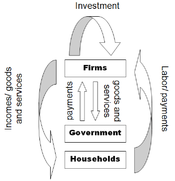
  Figure 1: The illustration of money/goods and services flows in an economy

  There are three ”players” in an ”economy game”: households that consume goods and services spending the money earned by working in firms, firms who are renting labor from workers to produce goods and services and a government that purchases both goods and services. Hence, the total purchases of goods and services (i.e. demand $Z$) is composed of the household consumption, firm investments and government purchases of goods and services.

• autonomous expenditures $A=A(t)$ - expenditures independent from the total income in economy (total income is the amount of money earned by the individuals in economy), i.e. whatever the economic performance of the economy is, these money will be spent (e.g. government expenditures to keep the roads functional). Note that product $Y$ (which is expressed in monetary units) is identified with total income in the economy.

2.1 The Phillips model of business cycle

In the Phillips model of business cycle (developed in 1954), which from the physicist’s point of view is interesting by the methodology used, the product function $Y(t)$ is deduced from the observed and presumed relationships between the above mentioned characteristics of the economy (see e.g. [11]):

1. The total demand in economy $Z(t)$ is composed of the consumption of households $C=(1-s)Y$, $s=const$, investments purchases $I$ and the autonomous expenditures $A$ (we will consider it to be a given constant of government spending):

   $$Z=(1-s)Y+I+A,$$ (1)

2. The demand in economy can be satisfied only via the product of the economy (since we do not take into account other economies). Hence, ideally the demand $Z$ should be equal to supply (product) $Y$ in any time. But it is assumed (and more realistic) that the product $Y$ is reacting to the demand with a delay. For example if there is a demand for some fashionable consumer article and there is a lack of it in shops, the producers can react and increase its production, but this will take some time. Thus the supply of the article reflects the past demand. In this way also total product $Y$ ”persuades” the total demand $Z$ in time and, particularly in Phillips model it is assumed that the dynamics of product is given by

   $$\frac{{\rm d}Y(t)}{{\rm d}t}=\lambda(Z-Y),$$ (2)

   where $\lambda$ is a positive constant.

3. It is assumed that the potential investment $\tilde{I}(t)$ is depending on the product change in time $\tilde{I}(t)=v\frac{{\rm d}Y(t)}{{\rm d}t}$ ($v$ being constant), i.e. the investments are needed only if we want to increase production. For example if we want to produce more products in a factory, we will need more inventories, machines, etc. which generates the spendings falling within the ”investments” in the economic language. But the true investment $I(t)$ is delayed from the potential one, i.e. in reality the investments do not react on the change in product immediately (in our example we can imagine, that we begin product more products using more extensively the machines we already have and the new machines will be bought later). The change of true investments in time is then supposed to be proportional to the difference $(\tilde{I}(t)-I(t))$, i.e.

   $$\frac{{\rm d}I}{{\rm d}t}=\kappa\left(v\frac{{\rm d}Y(t)}{{\rm d}t}-I\right),$$ (3)

   where $\kappa$ denotes a positive constant.

Now the above mentioned equations describe the model of how business cycle come into existence: the product is delayed from demand, and investment purchases are delayed from their immediate need. These two factors generate in Phillips model the oscillations in time development of product $Y$. Combining equations (1-3) and eliminating $Z$ and $I$, we obtain a second-order differential equation for the unknown variable $Y$ which represents the business cycle:

$$\ddot{Y}+a\dot{Y}+bY=P,$$ (4)

where

$$a=\lambda s+\kappa(1-\lambda v)$$

$$b=\kappa\lambda s$$

$$P=\kappa\lambda A$$

are constant values. Equation (4) reminds us of forced oscillations under friction where $b=\omega_{0}^{2}$ is the square of the free oscillations frequency and $P$ is the external force acting on the system - generally it is a given function of time (this is the case also in Phillips model once the autonomous expenditure $A$ is not constant). In physics, the term $a\dot{Y}$, $a>0$, represents the damping arising when the surrounding medium exerts a resistance. In an economic system this term may cause both damped and explosive oscillations depending on the sign of $a$.

Solving the dynamical equation (4) for our economic problem, we can obtain harmonic oscillations, critical damping, damped or even explosive oscillation according to given parameters of the economic system. Given all the other parameters, by changing the constant $\lambda$ (which can be found in each of the constants $a,\,b,\,P$) we can obtain all types mentioned of time development of the system. The solution of (4) for several values of $\lambda$ can be found in Fig. 2.

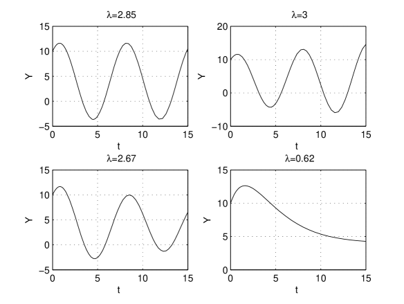
Figure 2: The solution of an unconstrained system; top-left: harmonic oscillations, top-right: explosive oscillations, bottom-left: damped oscillations, bottom-right:critical damping

Note that we do not mention concrete units in the graphs, since the results are derived for artificial parameters and for the purpose of demonstrating the behavior of the product $Y$. Visualizing ”non-specified” graphs is a standard means of qualitative presentation of economic behavior. But if needed, one can scale the product $Y$ in thousands of USD and the time axis in years.

The manner in which the product $Y$ is developing in time (harmonic, explosive, damped oscillations or the critical damping) depends on the particular choice of parameters $\kappa,\,\lambda,\,s,\,v,\,A$. Given the rest of parameters, the intervals of $\lambda$-values corresponding to each possible solution in Fig. 2 can be derived from a general solution of the dynamical equation (4). Analyzing these intervals, the economists conclude that oscillations, will occur if the time lag of product reaction to the demand does not differ significantly from the time lag of the reaction of investment to product change. The damped (explosive) oscillations will occur if the time lag of production to the demand will be significantly higher (lower) than the time lag of the reaction of investments to product change. These explanations following from the mathematical model answer the question of how the business cycle come to existence only to some extent. As we have mentioned there are many other approaches to business cycle modeling and always there may be a debate on the explanations and reasoning of each particular model.

It is worth noting that the final ”equation of motion” (4) for the economic system (we will call it a dynamical equation when talking about economic systems) was obtained based on assumptions (1-3) about the dynamic relationships among the economic quantities. But there is no mention about the Lagrangian of the economic system so as to generate the dynamic equation (4), nor are the terms in (4) interpreted as some economic ”forces”. Thus, although the resulting dynamical equation is well known in physics, the method of obtaining it lacks the systematic spirit of physical methodology (remember Lagrangian approach or Newton equations in mechanics.)

Hence, through certain assumptions Phillips model arrived to the description of oscillating behavior of product by the differential equation of second order. The ideal result of this model would be that once known the constants of the economy ($\lambda,\nu,s,\kappa,A$) one could predict the future oscillations of $Y$. Practically, the political authorities would prefer only steady economical growth (i.e growth of the product), which generates low unemployment, increasing wages and overall increasing life standard of people. Oscillations around this simple growth trend are disturbing and at least knowing how they come into existence or better, what they will look like next period, would bring important support to the policy makers. But as we have mentioned before, such predictions and even the understanding of the oscillation phenomena are not completed and are the subject of ongoing research.

Let us conclude the description of Phillips model of business cycle by the note that using the well-known and developed physical model (the harmonic oscillations) to describe observed economic behavior (product time development) was a natural initial approach in economics. Although the current philosophy of quantitative economics diverges fundamentally from simply adopting the existing physical models for the description of economic systems, the physical methodology itself is still in the focus of economists. Accordingly, the harmonic-oscillations-based methodology is still a common approach used for the description of economic systems nowadays (for a recent application see e.g.[12]). No matter how historical and simple the approach is, the Phillips model is able to produce at least qualitatively correct solutions (in the sense of correspondence with the observed behavior) as we shall see in Sec. 2.2.

2.2 Two interacting economies

In the preceding model we considered an isolated economy which had no contact with any other economy. In reality, economies are interacting through mutual purchases and money transfers. As typical in economics, a number of models were developed for this more realistic assumption. The most common is the model where, when describing a single economy, we introduce another ”player” (apart from households, firms and government) representing external economies influencing the economy modeled. But let us continue to develop a different, possibly more general, model employing the physical description initialized in the preceding section.

Let us consider economies of two countries which are ”interacting” through purchases and money transfers, i.e. part of the goods and services in an economy is purchased in the another. We can assume that the product in one economy will be affected besides other things also by the product of the other economy (for example if in Germany decreases the total product, i.e. there is less production of goods and services, then the demand of German firms for the sub-products and services imported from Czech Republic decreases and this will naturally affect negatively the product of Czech Republic. And, reciprocally, the less product in Czech Republic means lower income of households and lower consumption of all goods and services, among all those more expensive e.g. those imported from Germany, so the lower demand in Czech Republic will affect -to some extent- the German product).

Assume that, if there was no such interaction between the economies, each of them could be described in terms of equation (4). Hence, we can describe two economies without interaction as a system with two degrees of freedom using the dynamical equations:

$$\ddot{Y}_{1}+a_{1}\dot{Y}_{1}+b_{1}Y_{1} = P_{1},$$ (5)

$$\ddot{Y}_{2}+a_{2}\dot{Y}_{2}+b_{2}Y_{2} = P_{2},$$ (6)

with constants

$$a_{i}=\lambda_{i}s_{i}+\kappa_{i}(1-\lambda_{i}v_{i}),$$

$$b_{i}=\kappa_{i}\lambda_{i}s_{i},$$

$$P_{i}=\kappa_{i}\lambda_{i}A_{i},$$

where $i=1,2$ labels the economies. Following the physically motivated design of the Phillips model, we will formulate the interaction between the economies as a constraint binding the two coordinates ($Y_{1},\,Y_{2}$). In physics, the constraints are used if the real forces ensuring the observed behavior are not known or are uneasy to quantify. In a constrained system then, the constraint forces arise which ensure the prescribed behavior and have the meaning of real physical forces acting on the system (remember e.g. the rolling of the cylinder without slipping in mechanics where the constraint forces have the meaning of forces and torques stemming from interaction of the cylinder with underlay, see [13] or [14]). Although we have already mentioned that no ”forces” are defined in economics, the constraints seem to be an appropriate methodology since they make it possible to describe the really observed behavior whose ”dynamical generator” is not known. The relationship between the two economies can be stated generally as a nonholonomic constraint. For our artificial example, let us assume this constraint to be

$$\dot{Y}_{2}=k\dot{Y}_{1}+\alpha Y_{1}+\beta Y_{2},$$ (7)

where $k,\alpha,\beta$ are constants. Since the constraint is linear in velocities and the model itself is physically motivated, we will treat the constrained system in a way common in mechanics - we will use the nonholonomic approach (see e.g. [15] or [16]). Then, the dynamical equations for our constrained system take the form:

$$\ddot{Y}_{1}+a_{1}\dot{Y}_{1}+b_{1}Y_{1} = P_{1}-\mu k,$$ (8)

$$\ddot{Y}_{2}+a_{2}\dot{Y}_{2}+b_{2}Y_{2} = P_{2}+\mu,$$ (9)

which, together with constraint (7), yields 3 equations for 3 unknown variables $(Y_{1},Y_{2},\mu)$, where $\mu$ is the Lagrange multiplier. Eliminating the Lagrange multiplier from (8-9) and substituting from the constraint (7), we obtain reduced equations of the constrained system:

$$(1+k^{2})\ddot{Y}_{1}+A_{1}\dot{Y}_{1}++B_{11}Y_{1}+B_{12}Y_{2}-P_{1}-P_{2} = 0,$$ (10)

$$\dot{Y}_{2}-k\dot{Y}_{1}+\alpha Y_{1}+\beta Y_{2} = 0,$$ (11)

where

$$A_{1} = a_{1}+a_{2}k^{2}+\alpha k+\beta k^{2},$$

$$B_{11} = b_{1}+\alpha a_{2}k+\alpha\beta k,$$

$$B_{12} = \beta a_{2}k+kb_{2}+k\beta^{2}.$$

2.3 Results and discussion

Solving the constrained system (5-7) for three different sets of parameters $k,\,\alpha,\,\beta$ in (7):

Constraint A:	$\alpha=0$	$\beta=0$
Constraint B:	$\alpha=0.4$	$\beta=0.1$
Constraint C:	$\alpha=-0.1$	$\beta=-0.2$

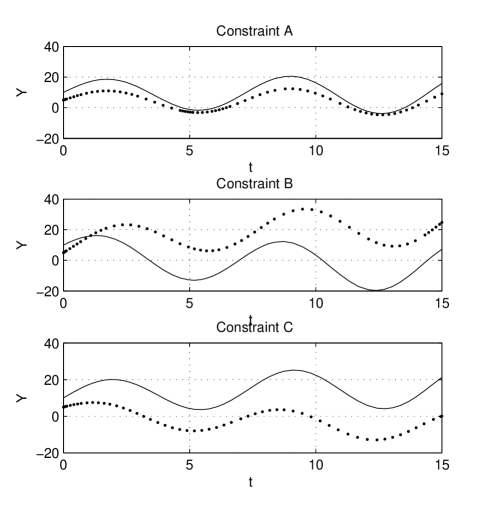
Figure 3: The solution of a constrained system for a particular setting of constraint parameters

we obtain the solutions in Fig. 3. The solutions provide qualitative information about product dynamics for two economies influencing each other. The particular time behavior of products $Y_{1},\,Y_{2}$ obviously depends on the particular form of the constraint. Note that, for realistic modeling, the particular coefficients $k,\,\alpha,\,\beta$ should be estimated from observed data. Since the qualitative results of the test case are for guidance only, we can state that, although being simple and based on an (old-fashioned) classical physically motivated model, the solution is in a qualitative correspondence with the observed behavior of the true interacting economies.

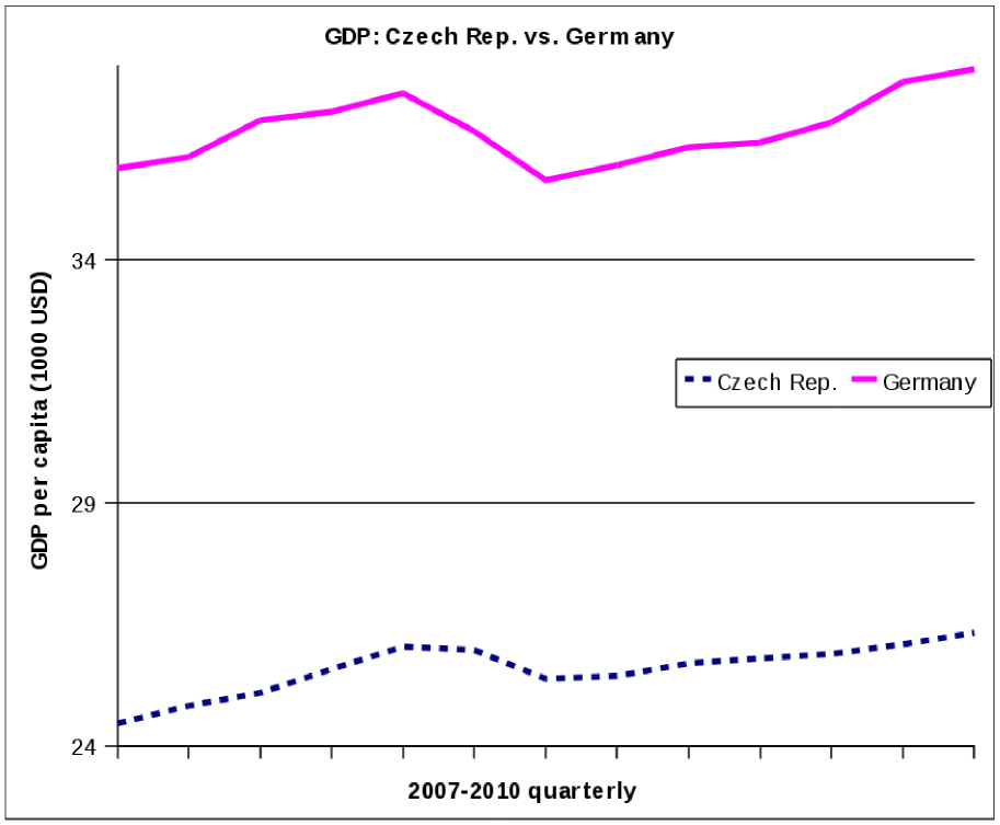
Figure 4: GDP per capita in Germany and Czech Republic: 2007 to 2010, quarterly (source: http://stats.oecd.org, expenditure approach, current prices, seasonally adjusted)

At Fig. 4 we can see the GDP time series of Czech Republic and Germany in the period 2007-2010. As we have already mentioned there is a considerable trading between these two economies which possibly make a connection between the time development of their products as qualitatively visible on Fig. 4. This connection could be qualitatively expressed by the constraint (7) and the model of two intercating economies (10-11) could enable to describe the business cycles of the two economies.

Thus, we have presented an example of how an economic model can be designed using the physical motivation. First the classical model of product dynamics based on the mechanical model of an oscillator was employed to describe an isolated economy. Then this model was extended to a model of two interacting economies using an oscillator-based approach, i.e. we treat each of the economies as a single component of the system with two degrees of freedom. The existing observed relationship between the economies was modeled by a constraint and the qualitative results of the model when compared to the real data (see Fig. 4) are promising. In economic science, such a model design could be successful after careful validation based on a concrete parameter estimation. As in other models, probably only some aspects of the observed behavior could be captured by the newly developed model and, therefore, a debate about the relevance of the assumptions made and the methodology used might be sparked. Nevertheless, such debates take place for any economic model no matter whether with a physical or other background. An important fact is that, so far, hardly any model has been validated in economics in the sense of physics, since there always can be found significant discrepancies between the data predicted by the model and those observed in the real economy world. Indeed, economic science is still trying to find the appropriate theories, methods and even the calculus to achieve the status of an unchallenged source of scholar knowledge.

3 The economic growth model using calculus of variations

While the short run variation in product (measured by gross domestic product -GDP- per capita ) is usually termed business cycle, the long run increase of per capita GDP is called economic growth. Economic growth is primarily driven by improvements in productivity, which involves producing more goods and services with the same inputs of labor, capital, energy and materials (therefore there is a lasting demand for innovations and technological improvements in developed economies). The long-run path of economic growth is one of the central questions of economics. An increase in GDP of a country greater than population growth is generally taken as an increase in the standard of living of its inhabitants, hence the aim of the policy makers is to achieve steady economic growth. To understand better the phenomena of economic growth and to obtain a quantitative support for making appropriate decisions a number of mathematical models of economic growth was developed during past fifty years. Again- as we have already mentioned when generally speaking about economic models- all models are representing the economic reality to individual extent and they differ in the assumptions made about how the economic characteristics are mutually interacting and influencing the final growth.

In this section, the Cass-Koopmans-Ramsey model of economic growth based on variational approach will be presented and the methodology and motivations behind an economic variational approach in comparison to traditional usage of variational calculus in mechanics will be investigated. Since the aim of this section is not to provide the reader with a thorough economical background of the model, we will describe the philosophy of the model intuitively (for more detailed notes about particular assumptions and economical background see e.g. [18]).

3.1 The Cass-Koopmans-Ramsey model

This time, there are two ”players” in the ”economy game”: firms and households (so the flows are similar to the previous model illustrated in Fig. 1 except the missing government purchases). The aim of the model is to answer the question of how much the product of economy at any point of time should be spent for immediate consumption to yield current utility, and how much of it should be saved (and invested) so as to enhance future production and consumption and, hence, yield future utility. The criterion of optimality is the social welfare which is given by social utility $U$. There are two time-dependent variables through which the desired optimal development of the economy can be attained: consumption $c(t)$ and capital $k(t)$ (measured in units advantageous for the model purposes, for details see [18]). Consumption represents the purchases of goods and services by households while capital is a factor of production, used to produce goods or services, that is not itself significantly consumed (though it may depreciate) in the production process (e.g. machinery, buildings, vehicles). Typically, in economics there is considered a relationship between the investment and the time derivative of the capital. In Cass-Koopmans-Ramsey model, the particular relationship takes the form

$$\dot{k}=f(k)-c-(n+g)k,$$ (12)

where $f(k)$ denotes the product (more precisely it is a known production function prescribing how the total production in economy is dependent on the capital available). Expression $f(k)-c$ has the meaning of investment and $(n+g)k$ is the amount of investment that must be done just to keep $k$ at its existing level ($n$ and $g$ being constants). The equation (12) states that the change in capital is equal to the investments less the replacement purchases (i.e. if we buy new machinery only to replace the broken ones then, even we made investments, we have not increased capital- we still have the same production factors for our production process as before the investment purchases.)

The task in Cass-Koopmans-Ramsey growth model is to maximize social utility $U(c)$ (which depends only on consumption) via time paths of variables $c$ and $k$ under the constraint (12). For the particular form of the utility function defined in Ramsey model (see [17] or [18]), we can write the overall optimization problem as:

$${\rm max} \hskip 28.45274ptU=\int_{0}^{\infty}Be^{-\beta t}\frac{c^{1-\theta}}{1-\theta}{\rm d}t$$ (14)

$$s.t.\hskip 17.07182ptf(k)-c-(n+g)k-\dot{k}=0,$$

where $B,\,\beta,\,\theta,\,n,\,g$ are positive constants with $0<\beta<1$. The form of the consumption function is the matter of intensive investigation and the particular form used in the Cass-Koopmans-Ramsey model represents just one approach. The term $e^{-\beta t}$ ensures discounting of economical quantities. It means that the flows of particular quantity (social utility in our problem) to come have smaller weight that its current flow. Note that this approach was doubted by many authors because by this model the priority is given to (our) current consumption at the expense of the consumption of future generations.

From the mathematical point of view this is a constrained variational problem with a velocity-dependent constraint (14). Solving (14-14), we obtain the optimal growth path, in other words, we realize how $c$ and $k$ must behave over time to achieve the maximal lifetime utility from the consumption flow given the relation (14) between the product, consumption and investment. Note that $c$ in (14) could be substituted from (14) to obtain an unconstrained variational problem with the Lagrangian dependent on both variable $k$ and its first derivative $\dot{k}$. Because the form (14-14) of the growth model is typically used in economics (thanks to its better economic interpretation and reasoning), we will not ”simplify” the initial problem (14-14) and it will be treated as a constrained variational problem for the solution of which the vakonomic approach will be employed. The Lagrangian for the constrained problem (14-14) takes the vakonomic form

$$L=Be^{-\beta t}\frac{c^{1-\theta}}{1-\theta}+\lambda(f(k)-c-(n+g)k-\dot{k}),$$ (15)

were $\lambda=\lambda(t)$ is the Lagrange multiplier. Considering three variables $(c,\,k,\,\lambda)$ instead of the initial pair $(c,\,k)$, we obtain the variational dynamical equations:

$$e^{-\beta t}c^{-\theta}-\lambda = 0,$$ (16)

$$\lambda\frac{{\rm d}f}{{\rm d}k}-(n+g)\lambda+\dot{\lambda} = 0,$$ (17)

$$f(k)-c-(n+g)k-\dot{k} = 0.$$ (18)

Note that the vakonomic approach accounts for the main technique used to solve variational constraint dynamical problems in economics (see [17],[18],[19] for typical examples). For the description and some notes on the comparison of vakonomic and nonholonomic approach see Appendix 1.

Figure 5: The dynamics of $c$ and $k$ in Ramsey model

3.2 Results and Discussion

Expressing $\lambda$ from (17) and substituting it into equation (16), we arrive after some calculation to a system of two equations for two unknown variables $c(t),\,k(t)$:

$$\frac{\dot{c}}{c} = \frac{\frac{{\rm d}f}{{\rm d}k}-\beta-n-g}{\theta}$$ (19)

$$\dot{k} = f(k)-c-(n+g)k.$$ (20)

Then, it is not difficult to find a solution to our problem, i.e. to find an optimal consumption and capital paths. Nevertheless, in economics the functions are not normally given explicitly, but only assumed to have characteristic qualitative properties (such as that the utility is an increasing non convex function of consumption). Thus the problems have an air of ”theory” rather than ”computation” and reaching a particular solution is neither possible nor necessary. Yet, the content of the problems is meaningful and analyzing the qualitative characteristics of the solutions often generates important insights into economic behavior. In models of economic dynamic optimization, two-variable diagrams are prevalently employed to obtain these qualitative analytical results.

The behavior of an economy in the Cass-Koopmans-Ramsey problem is typically described in terms of the evolution of $c$ and $k$ using a diagram at Fig. 5. This diagram reflects the dynamical equations (19-20) where the arrows show the directions of change of both $c$ and $k$. In mechanics, we can plot similar diagrams but this is mostly done for a particular solution. In such a case the trajectory of the system in the configuration space is obtained. The diagram in Fig. 5 is used to identify the qualitative optimal behavior of an economy given the initial conditions and additional requirements (such as $k\geq 0$). Then, the result consists in a verbal description of the optimal behavior rather then in an analytical solution. As an example, let us discuss the top left ”quadrant” of the graph. The consumption in economy is high and rising and $k$ eventually reaches zero. When $c$ continues to rise $k$ must become negative. But this cannot occur. Since the product is zero when $k$ is zero, the consumption must drop to zero. Therefore, such paths can be ruled out from consideration about realistic behavior of an economy. In a similar way, other ”quadrants” in Fig. 5 can be analyzed and we would arrive to a conclusion that the possible time path of the system is the one driving into the point where $\dot{k}=0,\,\dot{c}=0$. Then the economy is said to ”move along the saddle path” to the equilibrium in $\dot{k}=0,\,\dot{c}=0$. The equilibrium is Pareto-efficient which means that it is impossible to make anyone better off without making someone else worse off. The explanation lies in the fact that all the households in the model have the same utility. The equilibrium produces the highest possible utility among allocations of capital and consumption that treat all households in the same way. Once the economy arrives to this equilibrium it can not do better and therefore we do not change the level of capital and consumption anymore, i.e. $\dot{k}=0,\,\dot{c}=0$ (for details see [18]).

We can see clearly the difference between the application of variational calculus in mechanics where we are searching for a particular solution which prescribes the time evolution of the system precisely, and the economic application, where the behavior of the system is only qualitatively analyzed.

3.3 Lagrange multiplier interpretation

A first look at a nontrivial constrained optimization economic problem may be surprising for the student of physics. Leaving aside the unusual definition of feasible region in economic optimization problem (mostly restricted to non-negative values of variables), the economic interpretation of the Lagrange multiplier is worth a discussion. Mathematical texts provide no interpretation of the Lagrange multiplier $\lambda$, leaving the student with the impression that $\lambda$ has no significance beyond providing an extra variable which transforms a constrained problem into an unconstrained, higher dimensional one. But in economic problems, the Lagrange multiplier can usually be interpreted as the rate of change of optimal value of the criterion function relative to some parameter.

The constraint (14) describes the capital accumulation and thus $\lambda$ should correspond to the value of having a tiny bit more capital (see Appendix 2 for simple explanatory example). Hence, we can find the meaning of the Lagrange multiplier by answering the question of how the unit change in capital available in economics will affect the utility in optimum. Let us derive the influence of change in capital onto a ”present value” instantaneous utility $\bar{u}=u(c)e^{-\rho t}$ (see (14)):

$$\frac{{\rm d}\bar{u}}{{\rm d}k}=\frac{\partial\bar{u}}{\partial k}+\frac{\partial\bar{u}}{\partial c}\frac{\partial c}{\partial k}.$$ (21)

From the first variational dynamical equation (16) we obtain

$$\lambda=\frac{\partial\bar{u}}{\partial c},$$ (22)

and differentiating the constraint (18) we get

$$\frac{\partial c}{\partial k}=\frac{\partial f}{\partial k}-(n+g).$$ (23)

Substituing into relation (21) from (22-23) and having on mind that $\frac{\partial\bar{u}}{\partial k}=0$, we obtain

$$\frac{{\rm d}\bar{u}}{{\rm d}k}=\lambda\left(\frac{\partial f}{\partial k}-(n+g)\right).$$ (24)

That is, the extra unit of capital will raise the flow of output by an amount $\partial f/\partial k$ each unit of which (without the unit replacement production $n-g$ needed for keeping the capital at existing level and thus not intended for consumption) has a utility value of $\lambda$. Multiplier $\lambda$ is referred to as a shadow value of capital (evaluated in present value). New economical interpretation arises then from variational equation (16) and (22), respectively: It states that the marginal utility of consumption is equal to the shadow value of capital, $\lambda$. Thus, at the optimum the consumer is indifferent between consuming an additional unit and investing it. Remember, that the consumer must decide whether to consume or to save (which directly generates the investments) additional unit (of income). If it is consumed it brings direct utility, if it is invested (into capital) then it increases the product and future consumption. If the marginal utility of consumption was larger than the shadow value of capital,

$$\frac{\partial\bar{u}}{\partial c}>\lambda,$$ (25)

then capital would be too high and consuming more and saving less would increase the utility. Similarly, if the marginal utility of consumption was lower that the shadow value of capital

$$\frac{\partial\bar{u}}{\partial c}<\lambda,$$ (26)

then capital is too low and the households should save more to increase utility through higher future consumption. This example of Lagrange multiplier interpretation together with the subsequent discussion of dynamic equations represent the typical approach of optimization problem analysis in economics.

In mechanics, no interpretation is used for multipliers in optimization problems, but remember that the multipliers arise in the constrained forces, which are important from the physical point of view. The concept of constrained forces, on the other hand, has no significance in economic problems although the multipliers do. Hence, although the computational routine remains similar, there are distinct interpretations of the tools used.

4 Conclusion

Classical mechanics has played a significant role in the development of economic thinking influencing it in both principles and the calculus. Currently, different attitudes to the adoption of physical methodology for economic purposes can be distinguished. A strong one supports the philosophy that applying the well developed physical methods could quickly provide the economists with working and applicable models. This strong motion in economic science is reflected by a newly arisen term ”econophysics” which currently designates one of the possible fields where the undergraduates and graduates of physics could be involved.

The examples presented in the paper enable the undergraduates to meet for the first time this highly modern and progressively expanding field, and to get in touch with different philosophy of building scholar knowledge in economics. These examples may serve as a motivation for students to further study the economics - mechanics (or more generally physics) intersections. In addition, studying these problems makes the undergraduate students of physics face the different usage of a known methodology: the constraint variational calculus appears to be a flexible approach which in each discipline provides specific information and the nonholonomic dynamics of systems, based on constraint forces, could be applied even outside mechanics.

In physics education, the economic examples presented can serve not only as a demonstration of interdisciplinary applications of methods typically used in mechanics, but can also provide the teachers with an aid for demonstrating what are general mathematical and what are specifically physical features of the mechanics methodology. In this way, the students can achieve a deeper insight into the physical background of what they have learned in classical mechanics courses.

$$\frac{\partial L}{\partial q}-\frac{{\rm d}}{{\rm d}t}\frac{\partial L}{\partial\dot{q}}=\left(\frac{\partial f}{\partial\dot{q}}\right)^{T}\cdot\mu,$$ (27)

$$f(t,q,\dot{q})=0,$$ (28)

where $\mu$ are the Lagrange multipliers. The nonholonomic approach is typically used for solving the mechanical systems with nonholonomic constraints although in mechanics the non-holonomic constraints are frequently affine in velocities. The form of constraint forces for classical ideal constraints is a consequence of d’Alemberts principle. Note, that the nonholonomic approach has been extended also to more general constraints by the work of Chetaev [20] and others (see e.g. [21]; for instructive nonholonomic mechanical problems see e.g. [13], [16], [14]).

The mathematical concept of nonholonomic dynamics had been kept essentially unchanged until 30 years ago when a new dynamics of velocity constrained mechanics system was introduced by Kozlov [22]. This new mechanics was called vakonomic being ”variational axiomatic kind”. If we adopt a variational approach by requiring the motion to be a stationary curve of the action functional among all curves having the same end points and satisfying the nonholonomic constraints, then we get a vakonomic motion, i.e. we search for the solution of (unconstrained) variational problem associated to the Lagrangian function

$$\bar{L}(t,q,\dot{q},\lambda,\dot{\lambda})=L(t,q,\dot{q})+\lambda f(t,q,\dot{q}).$$

Namely, the vakonomic motions can be obtained by the Lagrange equations

$$\frac{\partial\bar{L}}{\partial q}-\frac{{\rm d}}{{\rm d}t}\frac{\partial\bar{L}}{\partial\dot{q}}=0,$$ (29)

$$\frac{\partial\bar{L}}{\partial\lambda}-\frac{{\rm d}}{{\rm d}t}\frac{\partial\bar{L}}{\partial\dot{\lambda}}=0,$$ (30)

which give

$$\frac{\partial L}{\partial q}-\frac{{\rm d}}{{\rm d}t}\frac{\partial L}{\partial\dot{q}}-\left(\frac{\partial f}{\partial\dot{q}}\right)^{T}\cdot\dot{\lambda}+\left(\frac{\partial f}{\partial q}-\frac{{\rm d}}{{\rm d}t}\frac{\partial f}{\partial\dot{q}}\right)^{T}\cdot\lambda=0,$$ (31)

$$f(t,q,\dot{q})=0.$$ (32)

Comparing the nonholonomic (27) and vakonomic equations (31) we arrive to a conclusion that the arising systems of differential equations are not equivalent unless

$$\frac{\partial f}{\partial q}-\frac{{\rm d}}{{\rm d}t}\frac{\partial f}{\partial\dot{q}}=0.$$

The author himself in [22] says: ”…vakonomic dynamics, which is an internally consistent model that can be applied to description of the motion of any mechanical systems, is as ”true” as traditional nonholonomic mechanics. The issue of the choice of model for each particular case is ultimately resolved by experiment.” While there are doubts that vakonomic dynamics is a satisfactory model for nonholonomic systems in mechanics (see e.g. [15]), in economics vakonomic approach is the one typically used for the solution of dynamical optimization problems with velocity dependent constraints. Intuitively, the nonholonomic concept based on the definition of constrained forces developed for mechanics could not be valid for the economic problems unless the background of the model is physically motivated. The vakonomic approach, if chosen for solving the constrained systems in economics, can be justified simply by the results it provides (for more examples on vakonomic approach in economics see e.g. [23], [24]).

Appendix 2

In constrained optimization in economics, the value of the Lagrange multiplier at the optimal solution is referred to as a shadow price. Shadow price is the change in the objective value of the optimal solution obtained by relaxing the constraint by one unit.

Consider a simple (static) business optimization problem of profit maximization in a firm. Assume that there are only two products and the firm is deciding about the amount of these two products $x_{1},\,x_{2}$ to be produced in next period. The profit and number of working hours needed per unit of each product are known and denoted by $a_{1},\,a_{2}$ and $l_{1},\,l_{2}$, respectively. The operating time limit for next period is $B$ (for example, we have B working hours available on certain machine for next month). We get the linear programming problem:

$${\rm max} \hskip 28.45274pt\pi=a_{1}x_{1}+a_{2}x_{2}$$ (34)

$${\rm s.t.}\hskip 17.07182ptl_{1}x_{1}+l_{2}x_{2}=B.$$

We introduce a multiplier $\lambda$ and form the Lagrangian

$$L=\pi+\lambda(B-l_{1}x_{1}-l_{2}x_{2}).$$

Assuming that the firm maximizes profit (given the constraint (34)), the optimal quantities $x_{1}^{\star},\,x_{2}^{\star}$ and the multiplier $\lambda^{\star}$ necessarily satisfy the first-order conditions:

$$\frac{\partial L}{\partial x_{1}} = \frac{\partial\pi}{\partial x_{1}}-\lambda l_{1}=0,$$ (35)

$$\frac{\partial L}{\partial x_{2}} = \frac{\partial\pi}{\partial x_{2}}-\lambda l_{2}=0,$$ (36)

$$\frac{\partial L}{\partial\lambda} = B-l_{1}x_{1}-l_{2}x_{2}=0,$$ (37)

and differentiation of constraint (34) yields

$$l_{1}\frac{\partial x_{1}}{\partial B}+l_{2}\frac{\partial x_{2}}{\partial B}=1.$$ (38)

Now, using the chain rule and equations (35), (36), (38) we obtain

$$\frac{\partial\pi}{\partial B}=\frac{\partial\pi}{\partial x_{1}}\frac{\partial x_{1}}{\partial B}+\frac{\partial\pi}{\partial x_{2}}\frac{\partial x_{2}}{\partial B}=\lambda l_{1}\frac{\partial x_{1}}{\partial B}+\lambda l_{2}\frac{\partial x_{2}}{\partial B}=\lambda.$$ (39)

Hence, the Lagrange multiplier $\lambda$ measures how the total profit responds to the unit change in total machine operating time available. The shadow price is here the maximum price the manager would be willing to pay for operating the production line for an additional unit of time, based on the benefits he would get from this change. For example, if $\lambda=1$ Euro, then running the machine and producing for an additional hour will gain the profit of $1$ Euro and the manager should not pay more for this additional working hour than is the value it produces (for more see e.g. [25]).

References

- [1] E. Ray Canterbery, A Brief History of Economics, World Scientific Publishing (2002).
- [2] Grattan-Guinness I, ”How influential was mechanics in the developement of neoclassical economics? A small example of a large question”, Journal of the History of Economic Thought 32, 531–581 (2010).
- [3] H. Stanley et al., ”Anomalous fluctuations in the dynamics of complex systems: From DNA and physiology to econophysics” Physica A 224, 302–321 (1996).
- [4] M. Schulz, Statistical physics and economics, Springer-Verlag New York, Inc., (2003).
- [5] I. Kitov, O. Kitov, Mechanomics: Economics as Classical Mechanics, Lap Lambert Academic Publishing (2010).
- [6] Ch. Schinckus, ”Econophysics and economics: Sister discipline?”, Am. J. Phys.78, 325–327 (2010).
- [7] A. Walstad, ” Comment on Econophysics and economics: Sister discipline?”, Am. J. Phys.78, 789–789 (2010).
- [8] D. Stauffer, ”Teaching computational bio-socio-econo-physics” Eur. J. Phys. 26, S79–S84 (2005).
- [9] P. Mostardinha, E.J. Durana, F.V. de Abereu, ”The econophysics in the Euromillions lottery”, Eur. J. Phys. 27, 675–684 (2006).
- [10] A. O’Sullivan, S. M. Sheffrin, Economics: Principles in action. Upper Saddle River, Pearson Prentice Hall (2003).
- [11] R.G.D. Allen, Mathematical economics, ST Martin’S Press INC, New York (1963).
- [12] A. Ataullah, M.Tippett, ”Equity prices as a simple harmonic oscillator with noise”, Physica A. 382, 557–564 (2007).
- [13] J. Janová, J. Musilová, J. Bartoš, ”Coupled rolling motion: a student project in non-holonomic mechanics,” Eur. J. Phys. 30, 1257–1269 (2009).
- [14] J.Janová, J. Musilová, ”The streetboard rider: an appealing problem in non-holonomic mechanics”, Eur. J. Phys. 31, 333–345 (2010).
- [15] G. Zampieri, ”Nonholonomic versus Vakonomic Dynamics”, J. Diff. Eq. 163, 335–347 (2000).
- [16] J. Janová, J. Musilová, ”Coupled rolling motion: considering rolling friction in non-holonomic mechanics,” Eur. J. Phys. 32, 245–257 (2011).
- [17] A.C. Chiang, Elements of dynamic optimization, Waveland Press, Inc. (2000).
- [18] D. Romer, Advanced macroeconomics, McGraw-Hill, (2006).
- [19] P. Aghion, P. Howitt, Endogenous growth theory, The MIT Press, Cambridge (Mass) (1998).
- [20] N.G. Chetaev ”On Gauss Principle” (in russian ), Izv. Kazan. Fiz. Mat. Obs.6, 323–326 (1932).
- [21] M. de Leon, D.M. de Diego, ”On the geometry of non-holonomic Lagrangian systems”, J. Math. Phys. 37, 1–26 (1996).
- [22] V. V. Kozlov, ”Dynamics of systems with nonintegrable constraints”, Part I, Moscow. Univ. Mech. Bull. 37 (1982), 27-34; Part II, 74-80, Part III 380 , 40–51 (1983).
- [23] A. Grubbstrom, ”Application of Calculus of Variations to Financing Alternatives”, Omega 19, 305–316 (1990).
- [24] A. Molinder, ”Application of calculus of variations to a continuous time aggregate production model”, Int. J. Prod. Econ. 41, 273–280 (1994).
- [25] J.V. Baxley, ”Lagrange Multiplier Problems in Economics”, Am. Math. Mon. 91, 404–412 (1984).