Monte Carlo study of the critical properties of the three-dimensional $120^{\circ}$ model

Abstract

We report on large scale finite-temperature Monte Carlo simulations of the classical $120^{\circ}$ or $e_{g}$ orbital-only model on the simple cubic lattice in three dimensions with a focus towards its critical properties. This model displays a continuous phase transition to an orbitally ordered phase. While the correlation length exponent $\nu\approx 0.665$ is close to the 3D XY value, the exponent $\eta\approx 0.15$ differs substantially from O(N) values. We also introduce a discrete variant of the $e_{g}$ model, called $e_{g}$-clock model, which is found to display the same set of exponents. Further, an emergent U(1) symmetry is found at the critical point $T_{c}$, which persists for $T<T_{c}$ below a crossover length scaling as $\Lambda\sim\xi^{a}$, with an unusually small $a\approx 1.3$.

1 Introduction

Orbital degrees of freedom are a key ingredient to the rich physics observed in many transition metal compounds, where in combination with magnetic and charge degrees of freedom complex phase diagrams are realized [1]. Several paradigm spin models have been introduced to describe the physics originating from the collective interplay of those orbital degrees of freedom. In their most pure form, these models are called orbital-only models neglecting all but orbital degeneracy [2, 3]. Beyond their original motivation, these models are also discussed in quite a different context, e.g. in connection to quantum information [4]. It is quite surprising, though, that despite their prototype status only little is known about the finite-temperature properties, and in particular about their critical properties and the precise nature of orbital-ordering thermal phase transitions in three-dimensions.

Here, we present results of a comprehensive Monte Carlo (MC) investigation of the nature of the finite-temperature phase transitions of the prototypical $120^{\circ}$ orbital-only model on the three-dimensional (3D) cubic lattice, complementing on our recent short account [5]. The $120^{\circ}$ model is the most basic model describing $e_{g}$ orbital degeneracy of electrons in the $d$-shell, hence the model is often also called the $e_{g}$ model. We study here the classical version because the corresponding quantum model has a sign problem precluding Quantum Monte Carlo approaches, and because in Ginzburg-Landau theory one typically expects quantum and classical versions of a same model to have the same critical properties, although exceptions are possible. For a detailed finite-temperature treatment of the three-dimensional compass model – the second major orbital-only model [3] – the reader is referred to a forthcoming publication [6].

2 Definition of the $120^{\circ}$ model

The $120^{\circ}$ or $e_{g}$ model (EgM) is defined by the Hamiltonian [3]

$$\mathcal{H}_{e_{g}}=-\ J\sum_{i,\alpha}{\boldsymbol{\tau}}_{i}^{\alpha}{\boldsymbol{\tau}}_{i+\mathbf{e}_{\alpha}}^{\alpha},$$ (1)

where $\boldsymbol{\tau}_{i}$ is an auxiliary three component vector obtained by an embedding of the orbital degree of freedom $\mathbf{T}_{i}=(T^{z}_{i},T^{x}_{i})=(\cos(\varphi),\sin(\varphi))\in S^{1}$:

$${\boldsymbol{\tau}}_{i}=\pmatrix{-1/2&\sqrt{3}/2\cr-1/2&-\sqrt{3}/2\cr 1&0}\mathbf{T}_{i}.$$ (2)

The $\boldsymbol{\tau}_{i}$ vector is therefore constrained onto a specific greater circle on $S^{2}$. The $\mathbf{e}_{\alpha}$ denote the positive unit vectors in the $\alpha\in\{x,y,z\}$ cartesian directions. Note that the coupling in $\boldsymbol{\tau}$-space depends on the spatial orientation of the bond. The coupling constant $J$ is set to one in the following, corresponding to ferromagnetic interactions. One the cubic lattice, results for antiferromagnetic interactions can be deduced from results using ferromagnetic couplings as the two cases can be mapped onto each other by a simple rotation of the pseudo-spins $\mathbf{T}$ on one sub-lattice [7].

For a long time, answering the question whether the EgM supports an orbital-ordered low-temperature phase, indicated by a local order parameter $\langle\mathbf{T}\rangle>0$, has been difficult due to the presence of a sub-extensive ground state degeneracy. However, a later rigorous analysis  [8, 9] showed that the ground state degeneracy is lifted at finite temperature by an order by disorder mechanism and that the EgM can indeed order into six discrete ordering directions, given by

$$\mathbb{T}^{o}_{n}=\left(\cos[n\ 2\pi/6],\sin[n\ 2\pi/6]\right),$$ (3)

with $n=0,\dots,5$. This analytical prediction was subsequently verified using classical MC simulations [10, 7], and at higher temperatures a continuous phase transition to a disordered phase has been found. Strikingly, no propositions concerning the universality class of this prototypical finite-temperature phase transition were made up until now, neither analytically nor numerically. Here, we will address this question and try to explore whether the special anisotropic interactions lead to new critical phenomena, as for instance found in dimer models [11, 12], or whether more conventional magnetic universality classes [13] describe the orbital-ordering transition.

3 Simulation technique, observables, and boundary conditions

The classical Hamiltonian (1) is considered here on a simple cubic lattice of side length $L$ and volume $N=L^{3}$. We perform state-of-the-art MC simulations along the lines of Refs. [14, 15], a key feature being the use of parallel-tempering methods as (so far) no cluster-like updates exist.

In order to detect long-range orbital ordering with $\langle\mathbf{T}\rangle>0$, possible order parameters are

$$m=(1/N)\sqrt{(\sum_{i}T^{z}_{i})^{2}+(\sum_{i}T^{x}_{i})^{2}},$$ (4)

which is the standard XY-order parameter, or alternatively

$$m=(1/N)\left|\sum_{i}T^{z}_{i}\right|+(1/N)\left|\sum_{i}T^{x}_{i}\right|.$$ (5)

Other order parameters are possible and were used [7]. In the following we use Eq. (5) in Sec. 4 and Eq. (4) in Sec. 5 to check the independence of our final results on the definition of the order-parameter. Moreover, the complementary quantity

$$D=(1/N)\sqrt{\left(E_{x}-E_{y}\right)^{2}+\left(E_{y}-E_{z}\right)^{2}+\left(E_{z\phantom{y}}\!\!-E_{x}\right)^{2}},$$ (6)

indicates a directional ordering of the bond energies and was previously studied in the compass model [16, 14, 15]. Here, $E_{x|y|z}$ is the total bond-energy along the ${x|y|z}$-direction (e.g., $E_{x}=-\ J\sum_{i}{\boldsymbol{\tau}}_{i}^{x}{\boldsymbol{\tau}}_{i+\mathbf{e}_{x}}^{x}$).

For the finite-size scaling study reported here, we shall further make use of the following quantities

$$\chi =N(\langle m^{2}\rangle-\langle m\rangle^{2}),$$ (7)

$$m^{\prime}_{\ln} =\mathrm{d}\ln m/\mathrm{d}\beta=N\left(\frac{\langle me\rangle}{\langle m\rangle}-\langle m\rangle\langle e\rangle\right),$$ (8)

$$m^{\prime} =\mathrm{d}m/\mathrm{d}\beta=N\left(\langle me\rangle-\langle m\rangle\langle e\rangle\right),$$ (9)

$$B_{m} =1-\langle m^{4}\rangle/3\langle m^{2}\rangle^{2},$$ (10)

denoting the susceptibility, the derivative of the logarithm of the order parameter, the derivative of the order-parameter, and the Binder parameter, respectively. Corresponding definitions apply to the order parameter $D$.

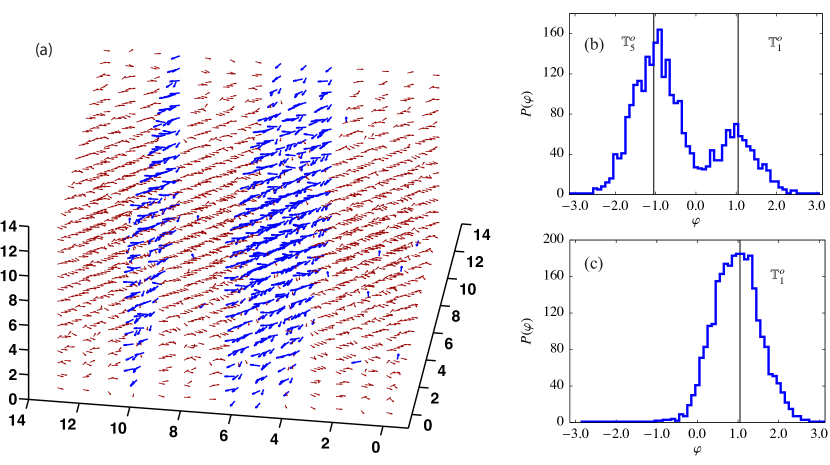
Figure 1: Analysis of spin configurations in the ordered phase ($T=0.4$) after thermalization. (a) A typical configuration in real space for $L=14$ and periodic boundary conditions where the small arrows indicate the pseudo-spins $\mathbb{T}$. Spins are color-coded according to their major orientation. A coexistence of two phases is apparent and the phase boundaries are more or less planar, possibly due to the planar gauge symmetries at $T=0$. (b) A typical histogram of the distribution of spin angles $\varphi$ of one configuration snapshot for $L=14$ and periodic boundary conditions showing incomplete ordering with contribution from collective ordering angles $\mathbb{T}^{o}_{1}$ and $\mathbb{T}^{o}_{5}$. (c) Similar histogram using screw-periodic boundary conditions which largely favor just one collective spin orientation (here $\mathbb{T}^{o}_{1}$ as indicated by the vertical line).

A few preliminary MC test runs employing periodic boundary conditions (PBC) clearly reproduce a signal of an ordered state at low-temperature and of a thermal phase transition in accordance with Ref. [7]. Moreover, by studying angular distribution functions $P(\varphi)$ of the pseudo-spin angle $\varphi$ after thermalization of a multitude of different initial configurations, clear evidence for a six-fold degenerate ordering is found. However, these initial runs also immediately reveal a couple of problems in the simulations, the most evident being the presence of incomplete ordering on small lattice sizes. This incomplete ordering is especially apparent by looking at a typical spin configuration [Fig. 1(a)] or at angular distributions of the spins (for one typical configuration) in a histogram [Fig. 1(b)] which show coexistence of ordering regions of different ordering angle $\mathbb{T}^{o}_{n}$. Such behavior is most likely due to the presence of the (gauge-like) planar reflection symmetries at $T=0$ [8] which are also responsible for the large ground-state degeneracy. For small system sizes, these reflections are still not too unfavorable energetically even at finite-temperatures. This problem could in principle be overcome by using an alternative order parameter like the one of Ref. [7] which is essentially insensitive to such ordering metastabilities. However, we additionally find that there are rather large finite-size corrections in any sort of scaling analysis on periodic boundary conditions.

Previously, we have shown for the 2D compass model that under the presence of gauge-like symmetries so-called screw-periodic boundary conditions (SBC) can be very favorable [15]. Indeed, SBC turn out to be very useful here as well: They naturally suppress metastable regions by gluing together different planes thereby favoring true collective ordering (visible in the histogram of Fig. 1(c)). Second and more importantly, they in principle allow to tune finite-size effects via the ”screw parameter” $S$. For points on the cubic lattice with coordinates $(x,y,z)$, SBC can be defined by

$$N_{x}(x,y,z)=\cases{(x+1,y,z)&if \quad$x<L-1$\\ (0,[y+S]\,\mathrm{mod}\,L,z)&if\quad$x=L-1$,}$$ (11)

where $N_{x}(x,y,z)$ denotes the nearest neighbor of $(x,y,z)$ in x-direction. This is one possible generalization of the definition given in Ref. [15]. A cyclic permutation is understood for the other cases (going in $y$ and $z$-direction). Here, we report results using $S=L/2$ which we empirically find to minimize finite-size effects.

4 Monte Carlo results and finite-size scaling for the $e_{g}$ model

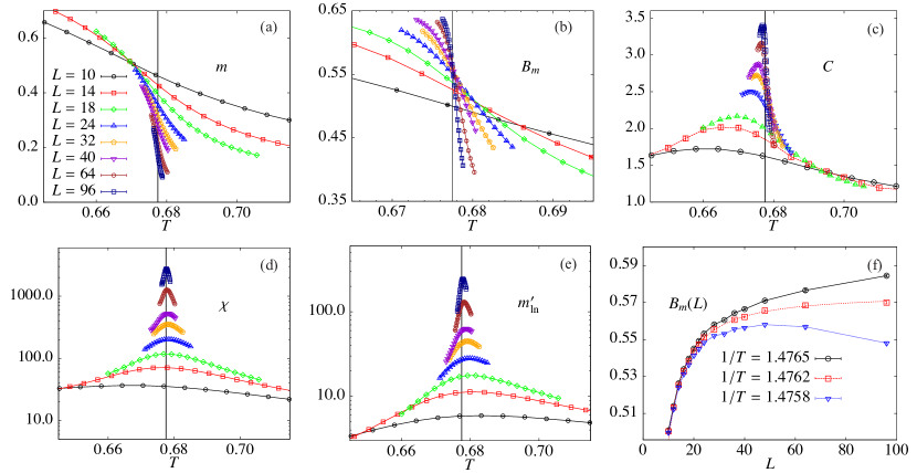
Figure 2: Monte Carlo results for the $e_{g}$ model close to the phase transition: (a) The order parameter $m$, (b) the associated Binder cumulant $B_{m}$, (c) the heat-capacity $C$, (d) the susceptibility $\chi$, and (e) $m^{\prime}_{\ln}$ as a function of temperature $T$ for different linear system sizes $L$. The vertical line indicates the location of the critical temperature $T_{c}$, obtained for example by an analysis of the finite-size scaling of $B_{m}(T_{c})$ according to Eq. (12) in (f).

We start by presenting numerical results for the EgM (1) with SBC on a couple of lattice sizes $L=8,\dots,96$. To obtain the reported accuracy, we collected at least $10^{6}$ or more independent MC measurements per data point. Figure 2 displays some pertinent data for the magnetization $m$ [using definition (5)], the Binder parameter $B_{m}$, the heat-capacity $C$, the susceptibility $\chi$, and for $m^{\prime}_{\ln}$ as a function of temperature $T$. All observables indicate a continuous phase transition at about $T_{c}\approx 0.677$, in agreement with earlier PBC estimates [10, 7]. A first precise estimate of $T_{c}$ can be obtained using the fact that $B_{m}(L)$ possesses only corrections to scaling at the critical point,

$$B_{m}(L)=B_{m}^{\star}+cL^{-\omega},$$ (12)

with $\omega$ being the correction exponent. Figure 2(f) shows that this scaling is very well satisfied for $T_{c}=0.6775$, and an effective $\omega\approx 1.4$ with a large constant $c$.

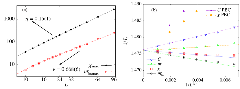
Figure 3: Finite-size scaling in the $e_{g}$ model: (a) Plot of $\chi_{\max}$ and $m^{\prime}_{\ln;\max}$ versus $L$ in a double logarithmic scale. Estimates for $\nu$ and $\eta$ where obtained from a finite-size study using Eq. (15) and Eq. (16), taking into account corrections to scaling. The dashed lines are the corresponding fit curves. (b)

Based on this, we now perform a finite-size scaling study to obtain the critical exponents. Here, we concentrate primarily on the correlation length exponent $\nu$ describing the divergence of the correlation length close to the critical point

$$\xi\sim\left|T-T_{c}\right|^{-\nu},$$ (13)

as well as the exponent $\eta$ governing the decay of the spin-spin correlation function

$$G(r)\sim r^{-d+2-\eta}$$ (14)

at the critical point. These exponents are determined using $m^{\prime}_{\ln;\max}=\max\{m^{\prime}_{\ln}\}$ and the maximum of the susceptibility, $\chi_{\max}=\max\{\chi\}$, which scale with system size $L$ as

$$m^{\prime}_{\ln;\max}\sim L^{1/\nu}(1+c_{m^{\prime}}L^{-\omega}),$$ (15)

$$\chi_{\max}\sim L^{2-\eta}(1+c_{\chi}L^{-\omega}).$$ (16)

Using the effective correction exponent $\omega$ obtained above based on the Binder cumulant, the data fits very well to Eq. (15) yielding our estimate

$$\nu=0.668(6)$$ (17)

for the correlation length exponent, see Fig. 3, which is roughly the same value as that of the universality class of the 3D XY model with $\nu_{\mathrm{XY}}=0.671$ [17, 18]. However, an analogous analysis of the order parameter correlations at criticality yields

$$\eta=0.15(1)$$ (18)

and provides strong evidence for a universality class distinct from the 3D XY class, which would yield a substantially smaller $\eta_{\mathrm{XY}}\approx 0.038$ [13, 17]. Our main results for the critical exponents have been reconfirmed by us using a slightly different but complementary analysis (using “running exponents”), without making use of $\omega$ [5].

Having found $\nu$, one can return once more to the question of the critical temperature which we want to obtain this time from the scaling of pseudo-critical temperatures $T_{c}(L)$, defined from the location of the peaks of the heat-capacity and of quantities defined in Eqs. (7),(8), and (9). Those pseudo-critical temperatures $T_{c}(L)$ should scale according to

$$T_{c}(L)=T_{c}+cL^{-1/\nu}(1+\cdots).$$ (19)

Figure 3(b) shows that such scaling is roughly satisfied for the largest system sizes and that all quantities converge to a unique $T_{c}$. We give our final estimate as

$$T_{c}=0.6775(1)$$ (20)

which is the mean of all extrapolations. This result is almost insensitive to slight changes in the exponent $\nu$ within the error bar. Moreover, similar data obtained on periodic boundary conditions [see Fig. 3(b)] converge to the same critical point but with evidently much larger finite-size effects, re-justifying the use of screw-periodic boundary conditions.

We remark that other critical exponents, like the exponent $\alpha$ for the specific heat, have been studied in a similar fashion. Our analysis yields $\alpha\approx 0$, which is in agreement with the usual hyper-scaling relation.

5 Monte Carlo results and finite-size scaling for the $e_{g}$-clock model

One might wonder whether the continuous nature of the orbital degrees of freedom $\mathbf{T}$ is necessary for the critical properties found. To address this question, let us consider here a naturally discretized version of Hamiltonian (1) – one in which the vectors $\mathbf{T}$ can only point along the six $\mathbb{T}^{o}$ ordering directions introduced above:

$$\mathcal{H}_{e_{g}}^{\circledast}=-\ J\sum_{i,\alpha}E^{\alpha}(n_{i},n_{i+\mathbf{e}_{\alpha}})\,.$$ (21)

Here, $E^{\alpha}(n_{i},n_{j})$ is the bond energy matrix along the bond direction $\alpha$ and $n=0,\ldots,5$ denote the six discrete onsite states $\mathbb{T}^{o}_{n}$. To be explicit, the following form of these matrices is easily obtained.

$$E^{x}(n,n^{\prime})=\frac{1}{4}\pmatrix{-4&-2&2&4&2&-2\cr-2&-1&1&2&1&-1\cr 2&1&-1&-2&-1&1\cr 4&2&-2&-4&-2&2\cr 2&1&-1&-2&-1&1\cr-2&-1&1&2&1&-1}$$ (22)

$$E^{y}(n,n^{\prime})=\frac{1}{4}\pmatrix{-1&-2&-1&1&2&1\cr-2&-4&-2&2&4&2\cr-1&-2&-1&1&2&1\cr 1&2&1&-1&-2&-1\cr 2&4&2&-2&-4&-2\cr 1&2&1&-1&-2&-2}$$ (23)

$$E^{z}(n,n^{\prime})=\frac{1}{4}\pmatrix{-1&1&2&1&-1&-2\cr 1&-1&-2&-1&1&2\cr 2&-2&-4&-2&2&4\cr 1&-1&-2&-1&1&2\cr-1&1&2&1&-1&-2\cr-2&2&4&2&-2&-4}$$ (24)

Note that via the above bond matrices, we can introduce an interpolation between the EgCLM and the three-state Potts compass model [6, 16] by multiplying all but the matrix elements equal to $-1$ with a factor $\lambda\in[0,1]$. Such interpolation could be useful to study the crossover from a second-order phase transition to a first order transition found for the Potts compass model [6]. The similarity of our model to the 6-state ($Z_{6}$) clock model

$$\mathcal{H}_{Z_{6}}=-J\sum_{\langle i,j\rangle}\mathbb{T}^{o}_{n_{i}}\cdot\mathbb{T}^{o}_{n_{j}}$$ (25)

serves as a motivation to term $\mathcal{H}_{e_{g}}^{\circledast}$ the $e_{g}$-clock model (EgCLM) [5].

In addition to re-investigating critical exponents, we now also analyze the directional order parameter $D$ as introduced in Eq. (6). In an orbitally ordered state characterized by a finite $m$, $D$ is also finite, however the converse is not true. An illustrative example is given by the 2D compass model, where a gauge-like freedom forbids orbital ordering altogether [19], while $D$ orders at finite temperature [16, 14, 15].

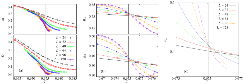
Figure 4: Monte Carlo data for the $e_{g}$-clock model: (a) Orbital order parameter $m(T)$ (upper panel) and directional order parameter $D(T)$ (lower panel) for different linear system sizes $L$. Note that both order parameters become finite below a common $T_{c}$ (indicated by the vertical line). (b) Binder parameters $B_{m}$ and $B_{D}$, and (c) the Binder parameter $B_{m}$ as obtained from simulations on periodic boundary conditions.

Due to its discrete nature, we were able to study larger systems of up to $L=128$ without much difficulty in our Monte Carlo runs. In addition, this allowed us to perform a more systematic comparison between periodic and screw-periodic boundary conditions. In Fig. 4, some of our resulting data is presented. Clearly, both $m(T)$ and $D(T)$ show an ordering tendency and both orbital ordering and directional ordering appear to set in at about the same temperature [see Fig. 4(a)]. In order to confirm the simultaneous onset we have in particular determined and compared the respective Binder parameters $B_{m}$ and $B_{D}$, see Fig. 4(b), indicating that both transitions take place at a unique critical temperature $T_{c}=0.67505(3)$. This result rules out a scenario of a directionally ordered, orbital-disordered intermediate phase, and establishes a single transition from a high temperature disordered phase to a low temperature orbitally ordered phase. It is at this place appropriate to study and compare the Binder parameter $B_{m}$ in more detail. At criticality, we note that $B_{m}(T_{c})\approx 0.589$ from the simulations on screw-periodic boundary conditions. Interestingly, on periodic boundary conditions the critical value of $B_{m}$ is much reduced to about $B_{m}(T_{c})\approx 0.41$, as shown in Fig. 4(c). Hence, there is a huge difference to the (weakly universal) value for $B_{m}\approx 0.586$ [20] found for the standard 3D XY model on periodic boundary conditions. Whether this large discrepancy is solely due to a distinct universality class as found here, or partly based on the directional nature of the ordered state remains to be investigated.

We now present our results for the critical exponents in the EgCLM, using the same scaling relations (15) and (16) as before. Figure 5 shows the finite-size scaling analysis and explicitly compares the scaling behavior for the two different boundary conditions. Most importantly, we obtain the same set of critical exponents as for the continuous $e_{g}$-model showing that just the nature of the ordered state, 6-fold degeneracy plus directional ordering, is relevant. Our most precise estimates $\nu=0.666(5)$ and $\eta=0.15(1)$ are taken from SBC. Prior to fitting, we have analyzed the critical Binder parameter yielding roughly the same effective correction exponent as before. The corresponding data for PBC show much larger finite-size effects (strong curvature in the log-log plot) but nevertheless give the same set of exponents. To reinforce our findings and to check our procedure, we also performed an analysis of the largely similar $Z_{6}$-clock model yielding exactly the 3D XY values as predicted [21, 22].

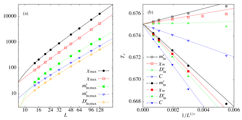
Figure 5: Finite-size scaling in the $e_{g}$-clock model. (a) Study of the exponents $\nu$ and $\eta$ according to Eqs. (15) and (16). Open symbols are from simulation with screw-periodic boundary conditions while filled symbols are obtained using periodic boundary conditions. The latter suffer from larger corrections to scaling as evident from the curvature (in this log-log plot). (b) Scaling of the pseudo critical temperatures using $\nu=0.666$. Both the data from SBC (open symbols) and from PBC (filled symbols) nicely converge to the same critical point $T_{c}$.

Note that an analysis based on the order parameter $D$ instead of $m$ leads to the same $\nu$ exponent (e.g. from $D^{\prime}_{\ln;\max}$ in Fig. 5(a)), while the corresponding $\eta_{D}$ exponent is much larger $(\approx 1.4)$. This simply follows from the assumption that $D$ has no intrinsic critical behavior, because then $D$ is driven by $m$: $D\sim m^{2}$, resulting in an apparently different $\eta$ value.

Last, we show a determination of the critical temperature from an scaling analysis according to Eq. (19) as shown in Fig. 5(b). Again, multiple observables and boundary conditions converge nicely to $T_{c}=0.67505(3)$. Interestingly, the $T_{c}$ for the discrete model is slightly smaller than that of the continuous variant. This observation can tentatively be explained by the fact that ordered phase is stabilized entropically.

6 Emergence of a U(1) symmetry

In the last part of this presentation we study the order-parameter distribution close to the critical point: In the ordered phase, a six-fold degeneracy is present and it is interesting to see how this structure is destroyed upon going into the disordered phase. To this end, we record histograms of the two-dimensional distribution $P(m_{x},m_{y})$, where $m_{x}=(1/N)\sum_{i}T^{z}_{i}$ and $m_{y}=(1/N)\sum_{i}T^{x}_{i}$ (i.e., the components of the vector order parameter $\langle\mathbf{T}\rangle$). The same distribution in polar coordinates is denoted by $P(r,\varphi)$. Fig. 6(a-c) shows a sequence of histograms for a relatively large system $L=64$ obtained from simulations of the EgCLM. In the ordered phase, the six-fold peak structure is recovered in the distribution function. However, at a temperature just below $T_{c}$ a continuous and uniform distribution with a finite radius shows up. This $U(1)$ symmetry of the orbital-order parameter is an emergent symmetry not present in the Hamiltonian, a situation largely reminiscent to the six-state $Z_{6}$ model, $Z_{q}$-perturbed XY models or the antiferromagnetic three-state Potts model [22, 23, 24]. Emergent $U(1)$ symmetries of discrete (i.e. dimer) order-parameters are also a major prediction of the theory of deconfined critical points [25, 26].

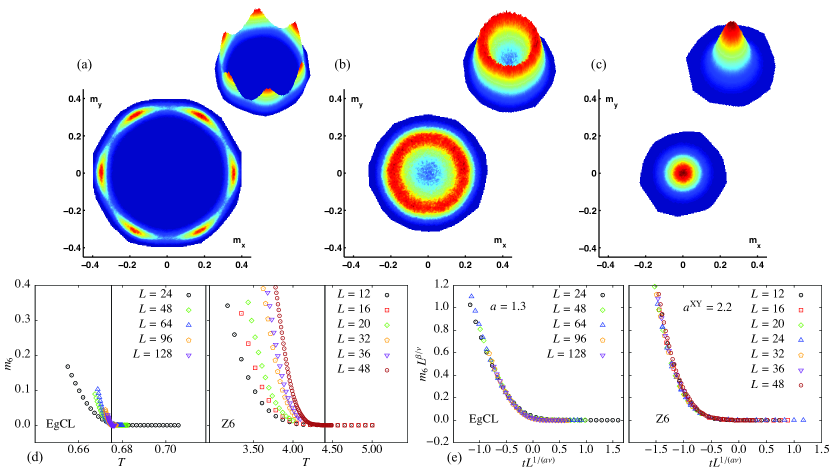
Figure 6: (a-c) Distribution functions $P(m_{x},m_{y})$ (histograms) of the order parameter obtained for $e_{g}$-clock model for $L=64$ in the ordered phase $(T=0.67)$, just below $T_{c}$ ($T=0.675$), and in the disordered phase $(T=0.68)$. In each case a top view and a tilted three-dimensional view is given to illustrate the form of the distribution functions. Values in the $z$-direction are shown on an arbitrary linear scale, which is therefore not shown. (d) The order parameter $m_{6}$ as defined in Eq. (27) for the $e_{g}$-clock model (EgCL) and the $Z_{6}$-clock model (Z6). For the EgCL, $m_{6}$ seems to become finite much more rapidly below $T_{c}$ (indicated by the vertical line) than in the Z6 case. (e) Collapse analysis of $m_{6}$: Best collapse parameters $a$ are indicated in the plot and differ clearly for the $e_{g}$-clock model and the $Z_{6}$-clock model.

The emergent $U(1)$ symmetry at the critical point continues to govern the order parameter below a crossover length scale $\Lambda$ below $T_{c}$ and this crossover scale is tied to the scaling of the correlation length $\xi$ via [21, 27, 28, 29]

$$\Lambda\sim\xi^{a},$$ (26)

with an exponent $a$ depending solely on the universality class of the critical point, at least in the case of $Z_{q}$-perturbed XY models [28, 29].

Hence, the value of $a$ defines another probe of unconventional critical behavior which we want to address here. In order to obtain $a$, one considers a modified order parameter

$$m_{6}=\int_{0}^{1}dr\int_{0}^{2\pi}d\varphi r^{2}P(r,\varphi)\cos(6\varphi),$$ (27)

which is sensitive only to the sixfold symmetry breaking, and which vanishes in the presence of a $U(1)$ symmetry [29]. Its finite-size scaling is thus influenced by $\Lambda$ rather than $\xi$, i.e. $m_{6}$ will be finite whenever the sixfold-structure is present in the histograms. In particular, it is argued that close to criticality the following scaling relations

$$m_{6}\sim L^{\beta/\nu}f(|t|L^{1/{a\nu}}),\quad m\sim L^{\beta/\nu}g(|t|L^{1/\nu})$$ (28)

hold, with $\beta$ being the critical exponent associated with the order-parameter, $t$ the reduced temperature, and $g$ and $f$ some scaling functions. Relations (28) allow to extract $a$ via a typical collapse analysis of $m_{6}$, ideally using a known value for $\beta/\nu$. We have performed this analysis both for the EgCLM and the $Z_{6}$ model as they have very similar ordered states, see Fig 6(d,e). In the case of the $Z_{6}$ model, we find $a^{XY}\approx 2.2$ (using $\beta/\nu=0.518$ for the 3D XY model). This result is consistent with the result of Ref. [29] but almost a factor two larger than the value $a\approx 1.3$ that we obtain for the EgCLM (using $\beta/\nu=(1+\eta)/2\approx 0.575$ for the 3D EG model). This result constitutes therefore further support for the unconventional critical behavior of the $120^{\circ}$ model found in other quantities.

7 Conclusions

We have studied the critical properties of the finite-temperature ordering transitions in the $e_{g}$ or $120^{\circ}$ model which plays a prototypical role in the study of collective effects resulting from orbital-degeneracy. Our systematic study points towards a distinct universality class for orbital-ordering, different from the standard (magnetic universality) classes we have encountered so far. Next to analyzing the original $e_{g}$ model, a discrete variant (the $e_{g}$-clock model) was defined and found to exhibit the same critical properties. In comparison to magnetic universality classes, unconventional critical properties are most apparent in the critical exponent $\eta$, describing the critical correlation function, and in the scaling of the length-scale $\Lambda$ related to the emergent $U(1)$ symmetry of the order parameter at the critical point. Our work provides a possible explanation of the unconventional observations made in the presence of impurities in the $e_{g}$ model [10]. Further theoretical work will be required to shed light on our findings and to understand in more detail the peculiar effects of the coupling of real space and order parameter space [13, 30], which are at work in the $120^{\circ}$ model. Recently, (artificially engineered) orbital systems became available in solids [3, 31, 32] which gives promising hope that the peculiar critical properties uncovered in the present work can be further explored experimentally.

References

- [1] Tokura Y and Nagaosa N 2000 Science 288 462
- [2] Khomskii D and Mostovoy M 2003 J. Phys. A: Math. and Gen. 36 9197
- [3] van den Brink J 2004 New J. Phys. 6 201
- [4] Douçot B, Feigel’man M, Ioffe L and Ioselevich A 2005 Phys. Rev. B 71 024505
- [5] Wenzel S and Läuchli A M 2011 Phys. Rev. Lett. 106 197201
- [6] Wenzel S and Läuchli A M 2011 unpublished
- [7] van Rynbach A, Todo S and Trebst S 2010 Phys. Rev. Lett. 105 146402
- [8] Nussinov Z, Biskup M, Chayes L and J van den Brink 2004 Europhys. Lett. 6 990
- [9] Biskup M, Chayes L and Nussinov Z 2005 Commun. Math. Phys. 255 253
- [10] Tanaka T, Matsumoto M and Ishihara S 2005 Phys. Rev. Lett. 95 267204
- [11] Alet F, Misguich G, Pasquier V, Moessner R and Jacobsen J 2006 Phys. Rev. Lett. 97 030403
- [12] Charrier D and Alet F 2010 Phys. Rev. B 82 014429
- [13] Pelissetto A and Vicari E 2002 Phys. Rep. 368 549
- [14] Wenzel S and Janke W 2008 Phys. Rev. B 78 064402
- [15] Wenzel S, Janke W and Läuchli A M 2010 Phys. Rev. E 81 066702
- [16] Mishra A, Ma M, Zhang F C, Guertler S, Tang L H and Wan S 2004 Phys. Rev. Lett. 93 207201
- [17] Campostrini M, Hasenbusch M, Pelissetto A, Rossi P and Vicari E 2001 Phys. Rev. B 63 214503
- [18] Campostrini M, Hasenbusch M, Pelissetto A and Vicari E 2006 Phys. Rev. B 74 144506
- [19] Nussinov Z and Fradkin E 2005 Phys. Rev. B 71 195120
- [20] Hasenbusch M and Török T 1999 J. Phys. A: Math. Gen. 32 6361
- [21] José J V, Kadanoff L P, Kirkpatrick S and Nelson D R 1977 Phys. Rev. B 16 1217–1241
- [22] Hove J and Sudbø A 2003 Phys. Rev. E 68 046107
- [23] Gottlob A P and Hasenbusch M 1994 Physica A: Statistical Mechanics and its Applications 210 217 – 236 ISSN 0378-4371
- [24] Heilmann R, Wang J S and Swendsen R 1996 Phys. Rev. B 53 2210
- [25] Senthil T, Vishwanath A, Balents L, Sachdev S and Fisher M 2004 Science 303 1490
- [26] Sandvik A W 2007 Phys. Rev. Lett. 98 227202
- [27] Blankschtein D, Ma M, Berker A N, Grest G S and Soukoulis C M 1984 Phys. Rev. B 29 5250–5252
- [28] Oshikawa M 2000 Phys. Rev. B 61 3430–3434
- [29] Lou J, Sandvik A W and Balents L 2007 Phys. Rev. Lett. 99 207203
- [30] Nattermann T and Trimper S 1975 J. Phys. A: Math. Gen. 8 2000
- [31] Jackeli G and Khaliullin G 2009 Phys. Rev. Lett. 102 017205
- [32] Chaloupka J, Jackeli G and Khaliullin G 2010 Phys. Rev. Lett. 105 027204