energies of knot diagrams

Abstract.

We introduce and begin the study of new knot energies defined on knot diagrams. Physically, they model the internal energy of thin metallic solid tori squeezed between two parallel planes. Thus the knots considered can perform the second and third Reidemeister moves, but not the first one. The energy functionals considered are the sum of two terms, the uniformization term (which tends to make the curvature of the knot uniform) and the resistance term (which, in particular, forbids crossing changes). We define an infinite family of uniformization functionals, depending on an arbitrary smooth function $f$ and study the simplest nontrivial case $f(x)=x^{2}$, obtaining neat normal forms (corresponding to minima of the functional) by making use of the Gauss representation of immersed curves, of the phase space of the pendulum, and of elliptic functions.

Introduction

In this paper, we introduce certain energy functionals defined on (a special class of) knot diagrams. Intuitively, these functionals correspond to (i.e., are mathematical models of) a thin (but not infinitely thin) knotted resilient wire constrained between two parallel planes.

The idea of defining energy functionals for classical knots is due to H. K. Moffat [9]. It was further developed by W. Fukuhara [4], J. O’Hara in [10], [11], [12], [13], M. H. Freedman, and Z.-X. He in [2], M. H. Freedman, Z.-X. He, and Z. Wang in [3] and together with S. Bryson in [1], D. Kim, R. Kusner in [8], O. Karpenkov in [5], [6] and others. The main underlying idea is to define a real-valued functional on the space of knots so that gradient descent along the values of the functional does not change the ambient isotopy class of the knot and leads to a well-defined minimum, which may be regarded as the normal form of the knot (corresponding to the given functional); if this gradient descent leads to the same normal form starting from any two knots in the same ambient isotopy class, we would have a solution of the knot classification problem – knots would be entirely classified by their normal forms.

However, none of the functionals studied so far have achieved this ambitious goal, and most of the experts appear to be skeptical about the existence of such a functional. Nevertheless, the functionals considered, in particular the Möbius energy functional devised by J. O’Hara, possess some important properties, for example, computer experiments show (see [3]) that any knot diagram of the unknot is taken to the round circle via gradient decent along the values of the Möbius energy functional, but the claim that the unknot has a unique normal form (the circle) has not been proved.

The functionals studied in the present paper differ from those mentioned above in that they are defined on knot diagrams (rather than knots in 3-space), gradient descent for them is not invariant with respect to the Reidemeister $\Omega_{1}$ move (but is invariant with respect to $\Omega_{2}$ and $\Omega_{3}$), and the diagrams themselves are not curved lines (they are like very thin solid tori lying on the plane). The real life prototypes of these “thin solid flat knots” were resilient thin wires constrained between two parallel planes. They were studied experimentally by A. B. Sossinsky in [14].

Consider a tubular flat knot of length $2\pi$ and cross-section radius $\varepsilon>0$, $\varepsilon\ll 1$ (the last inequality means “as small as we need in the given situation”); the knot is constrained between two parallel planes at a small distance (say $6\varepsilon$) from each other. Let us supply the core $K_{0}$ (central line) of our knot $K$ with an energy functional $E$ consisting of two summands:

$$E=U+R.$$

The functional $U$, which we shall call a uniformizational functional, serves to bring the core (via gradient descent) to a “perfectly rounded off” form. In this paper we consider a family of functionals depending on arbitrary continuous function $f$,

$$U_{f}(\gamma)=\int\limits_{S^{1}}f(\kappa(\gamma(t)))dt,$$

where $\kappa(\gamma(t))$ is the oriented curvature at the point $\gamma(t)$. The summand $R$ (which we call the resistance functional) forbids to perform deformations under which the knot type of the diagram changes (in particular, it forbids crossing changes). We define it as follows

$$R(\gamma)=\sum\limits_{\ell\in\operatorname{Alt}(\gamma)}\frac{1}{A(\ell)},$$

where the sum is taken over all cycles in knot diagrams bounding a disk and such that in their consecutive intersections overpasses and underpasses alternate (we refer to Subsection 2.1 for the exact definitions), and by $A(\ell)$ we denote the area of the cycle $\ell$. Further (in Subsections 2.2 and 2.3), we introduce two modification of this functional that are easy to compute.

This paper is organized as follows.

In the first section, we study the uniformization functionals. In Subsection 1.1, we define the family of uniformization functionals $U_{f}(\cdot)$. In Subsection 1.3, we show how to calculate the minima of these functionals by using the Gauss representation of regular curves described in Subsection 1.2. In Subsection 1.4, we perform such calculations for the particular case in which the function $f$ is given by $f(x)=x^{2}$. It turns out that the critical curves are related to the trajectories of pendulum. We prove that all the critical trajectories are either circles passed several times, or $\infty$-shaped curves (defined by elliptic functions) passed several times.

Section 2 is dedicated to resistance functionals. We start with the general notion of resistance energy in Subsection 2.1. In Subsections 2.2 and 2.3, we show how to simplify the complexity of resistance energy (material resistance energy and its genericity modification). In Subsection 2.4, we show that a regular deformation of bounded genericity energy preserves the knot type. Finally, in Subsection 2.5, we say a few words about the influence of material resistance energy on the shape of the normal form in the pendulum case (i.e., for $f(x)=x^{2}$).

In the brief concluding Section 3, we discuss the perspectives of this research and present some conjectures.

1. On the uniformization of regular curves

In this section, instead of knot diagrams, we consider regular $C^{2}$-curves of constant length $2\pi$ in the plane, in particular regular curves, construct various functionals on the space of such curves and investigate the normal forms given by the functionals. Gradient descent along these functionals tends to make the local structure of the curves more uniform (in a sense related to their curvature), and so we call them uniformization functionals.

1.1. A general family of uniformization functionals

Let $f$ be a real continuous function satisfying $f(0)=0$. A uniformization functional $U_{f}$ associated with the function $f$ is the functional defined at a regular $C^{2}$-curve $\gamma$ (with arclength parameter $t$) as follows

$$U_{f}(\gamma)=\int\limits_{S^{1}}f(\kappa(\gamma(t)))dt,$$

where $\kappa(\gamma(t))$ is the oriented curvature at the point $\gamma(t)$.

Example 1.1.

In the case when $f(x)=x$, the resulting functional is constant on regular homotopy classes of regular $C^{2}$-curves and equal to the Whitney index of the curve, i.e., the number of revolutions performed by the tangent vector to the curve as its initial point goes once around the curve.

Let us expand the definition of uniformization functionals to the broader class of curves for which $\kappa(\gamma(t))$ is not defined at all points of the given curve.

Definition 1.2.

Let $f$ be a positive continuous function satisfying $f(0)=0$. The extended uniformization functional $\hat{U}_{f}$ associated with the function $f$ is the functional defined at a regular $C^{2}$-curve $\gamma$ (with arc length parameter $t$) as follows

$$\hat{U}_{f}(\gamma)=\lim\limits_{\varepsilon\to 0}\frac{1}{\varepsilon}\int\limits_{S^{1}}f\bigg{(}\frac{1}{R\big{(}\gamma(t{-}\varepsilon),\gamma(t),\gamma(t{+}\varepsilon)\big{)}}\bigg{)}dt,$$

where $R(\gamma(t-\varepsilon),\gamma(t),\gamma(t+\varepsilon))$ is the radius of the circle passing through the points $\gamma(t-\varepsilon)$, $\gamma(t)$, and $\gamma(t+\varepsilon)$.

The next assertion readily follows from compactness arguments.

Proposition 1.3.

For any $C^{2}$-regular curve $\gamma$,

$$\hat{U}_{f}(\gamma)=U_{f}(\gamma).$$

∎

It is natural to suppose that the first interesting family of functionals for further study is the class associated with functions of the form $x^{\alpha}$ for $\alpha>1$ (we shall say a few words later about the case $\alpha=2$ and its relationship to pendulum motions).

1.2. Gauss representation of regular curves

Consider a regular curve $\gamma$ of length $2\pi$ with arclength parametrization $t$. Consider a function $\alpha:[0,2\pi]\to\mathbb{R}$ such that

$$\dot{\gamma}(t)=(\cos\alpha(t),\sin\alpha(t)).$$

We then say that $\alpha$ is a Gauss representation of the regular curve $\gamma$. (Here and later by $\dot{g}$ we denote the derivative ${\partial g}/{\partial t}$.)

Suppose now that we are given a function $\alpha$. When does this function represent a regular curve? Let us briefly answer this question. Consider the following three conditions on $\alpha$. Since the curve is closed, we have the ”coordinate” conditions:

(1) $$\int\limits_{0}^{2\pi}\cos\alpha(t)dt=\int\limits_{0}^{2\pi}\sin\alpha(t)dt=0.$$

In addition we know that

(2) $$\alpha(0)=\alpha(2\pi).$$

Proposition 1.4.

If the above three conditions are satisfied, then the resulting curve is regular. ∎

1.3. Critical points of the energy functionals $U_{f}$

Let us study critical points of the energy functionals $U_{f}$. Notice that in the Gauss representation we have $\kappa=\dot{\alpha}$, so the functional is of the following form:

$$U_{f}(\alpha)=\int\limits_{0}^{2\pi}f(\dot{\alpha})dt.$$

Theorem 1.5.

Consider a $C^{2}$-regular curve $\gamma$ and a nonnegative $C^{2}$-function $f$ satisfying $f(0)=0$. Let $\alpha$ be the Gauss representation of $\gamma$. Suppose $\alpha$ is critical for $U_{f}(\gamma)$. Then there exist constants $C_{1}$ and $C_{2}$ such that $\alpha$ satisfies

(3) $$f^{\prime\prime}(\dot{\alpha})\ddot{\alpha}=C_{1}\cos\alpha+C_{2}\sin\alpha.$$

Proof.

Consider a variation $\alpha+h\beta$ with a small parameter $h$. First, notice the following. As we vary the closed curve, the variation $\alpha+h\beta$ satisfies conditions (1) above, i.e., the derivative $\frac{d}{dh}$ of the corresponding integral equals zero, which is equivalent to

(4) $$\int\limits_{0}^{2\pi}\sin(\alpha(t))\beta(t)dt=\int\limits_{0}^{2\pi}\cos(\alpha(t))\beta(t)dt=0.$$

Secondly, for the case in which $\alpha$ is a critical point, all the variations are zero. Hence

$$\int\limits_{0}^{2\pi}f^{\prime}(\dot{\alpha})\dot{\beta}dt=0,\quad\text{which is equivalent to}\quad\int\limits_{0}^{2\pi}f^{\prime\prime}(\dot{\alpha})\ddot{\alpha}\beta dt=0.$$

The last equation holds for any variation $\beta$ satisfying Equations (4); therefore, we obtain

$$f^{\prime\prime}(\dot{\alpha})\ddot{\alpha}=C_{1}\cos\alpha+C_{2}\sin\alpha,$$

where $C_{1}$ and $C_{2}$ are some constants. ∎

Remark 1.6.

Theorem 1.5 means that the minima of the functional $U_{f}$ may be found by solving (for $\alpha$) the differential equation (1) with the appropriate initial conditions. Then the values of $\alpha$ at such minima specify curves that may be regarded as normal forms of the given curve. This approach allows to obtain normal forms by direct computations not involving gradient descent along the values of the functional.

1.4. The case $f(x)=x^{2}$: the pendulum

Let $f(x)=x^{2}$, then Equation (3) becomes

$$\ddot{\alpha}=C_{1}\cos\alpha+C_{2}\sin\alpha.$$

After an appropriate Euclidean transformation, we obtain the equation for the simple pendulum

$$\ddot{\alpha}+\omega^{2}\sin\alpha=0$$

for some nonnegative constant $\omega$ whose physical meaning is as follows:

$$\omega=\sqrt{g/L};$$

here $L$ is the length of the pendulum, and $g$ is the gravitational acceleration.

There are trivial solutions whose trajectories are circles passed several times. They correspond to $\omega=0$. The others solutions are more complicated. Consider the case $\omega>0$. The law of the motion of the pendulum is described by the equation

$$\sin\frac{\alpha}{2}=\xi\operatorname{sn}(\omega t+t_{0}|\xi),$$

where $\operatorname{sn}$ is the Jacobi elliptic sine, whose value $\operatorname{sn}(u|k)$ is defined from the equation

$$\operatorname{sn}(u|m)=\sin\phi,$$

where $\phi$ is a solution of the equation

$$u=\int\limits_{0}^{\phi}\frac{dt}{\sqrt{1-m^{2}\sin^{2}t)}}.$$

The constants $t_{0}$ and $\xi$ are parameters. Basically $t_{0}$ is the starting time parameter on the curve, so without loss of generality, we put $t_{0}=0$. The parameters $\omega$ and $\xi$ essentially define the trajectory.

Let us answer the following question.

Question. Which trajectories $\{\alpha(t)|0\leq t\leq 2\pi\}$ defined by $(\xi,\omega)$ result in a closed differentiable curve $\gamma_{\alpha}$?

The answer to this question is as follows.

Theorem 1.7.

All critical curves of the functional are either circles passed several times, or $\infty$-shaped curves passed several times.

Let $K$ be the complete elliptic integral of the first kind, i.e.,

$$K(m)=\int\limits_{0}^{1}\frac{dt}{\sqrt{(1-t^{2})(1-m^{2}t^{2})}}.$$

Conjecture 1.

We conjecture that all $\infty$-shaped extremal curves are homothetic to the curve $\gamma_{\alpha}$ for $\alpha$ satisfying

$$\sin\frac{\alpha(t)}{2}=\xi\operatorname{sn}\Big{(}\frac{2rK(\xi)t}{\pi}\Big{|}\xi\Big{)},$$

where $r$ is a nonzero integer and $\xi\approx.90890856$ $($see Figure 2 (left)$)$.

We say a few words related to this conjecture in Remark 1.8.

1.4.1. Proof of Theorem 1.7 and construction of the $\infty$-shaped critical curve

Consider the phase portrait (with coordinates $(\alpha,\dot{\alpha})$) of a pendulum; we do not specify $\omega$, since all the phase spaces are similar (see Figure 1). There are two non-singular types of trajectories and three singular types.

Figure 1. The phase portrait of the pendulum.

Singular case. In the singular case, we have singular points of type $(2k\pi,0)$ (stable equilibrium) and $((2k{+}1)\pi,0)$ (unstable equilibrium) and all separatrices (nonperiodic motion of the pendulum). At the equilibrium points the angle $\alpha$ does not change, and hence $\gamma_{\alpha}$ is not closed. In the case of the separatrices we have

$$0<|\alpha(0)-\alpha(2\pi)|<2\pi.$$

Hence the corresponding curve is not differentiable at $\gamma_{\alpha}(0)=\gamma_{\alpha}(2\pi)$ even if it is closed. So in the singular case there are no closed differential curves $\gamma_{\alpha}$.

General case of full swing pendulum trajectories. The full swing pendulum trajectories are situated in the white regions of Figure 1. Let us show that in this case there are also no differentiable closed curves $\gamma_{\alpha}$.

Without loss of generality, we assume that $\alpha(0)=0$, and, therefore, $\alpha(2\pi)=2k\pi$ for some integer $k$ (since the tangent vectors at $t=0$ and $t=2\pi$ must coincide). It is quite easy to see that on the segments $[(2m+1/2)\pi,(2m+3/2)\pi]$, the value of the modulus $|\dot{\alpha}|$ is smaller than at the segments $[(2m-1/2)\pi,(2m+1/2)\pi]$. Hence the integral

$$\int\limits_{0}^{2\pi}\cos\alpha(t)dt$$

is nonzero, and therefore any such curve is not closed.

Swing pendulum trajectories that are not full. Such trajectories are represented by the ovals on the phase portrait in the gray regions of Figure 1. In this case we have several closed differential curves $\gamma_{\alpha}$.

Again without loss of generality, we suppose that $\alpha(0)=0$, and, therefore, $\alpha(2\pi)=0$ (since the pendulum never reaches the vertical position corresponding to unstable equilibrium). This is equivalent to the relation

$$\xi\operatorname{sn}(2\pi\omega|\xi)=\sin\frac{\alpha(2\pi)}{2}=0.$$

The solutions of the equation $\operatorname{sn}(a|b)=0$ are described as follows:

$$a=2rK(b)+2IsK(1{-}b),\qquad\hbox{for $r,s\in\mathbb{Z}$,}$$

where $I=\sqrt{-1}$.

We conjecture that there are no closed curves in the cases for which $s\neq 0$.

Remark 1.8.

In the major cases, when $s\neq 0$, we end up with solutions $a=a(r,s,b)$ that have nonzero imaginary parts. Surprisingly, for the case $r=s$ and $b=3$, the value of $a$, i.e.,

$$2r(K(2)+IK(3)),$$

seems to be integer (numerical calculations only show that the first 1000 digits after the decimal point are zero ). We conjecture that these cases occur not often enough to have yield new closed curves $\gamma_{\alpha}$.

Let us study the case $s=0$. Then

$$2\pi\omega=2rK(\xi),\qquad\hbox{for $r,\in\mathbb{Z}$,}$$

and so $\omega=rK(\xi)/\pi$. Now let us check the conditions for the curve to be closed. The first one is

$$\int\limits_{0}^{2\pi}\sin\alpha(t)dt=0.$$

It turns out that this condition holds automatically for even values of $r$ and does not hold for odd $r$:

$$\int\limits_{0}^{2\pi}\sin\alpha(t)dt=-\frac{1}{\omega^{2}}\int\limits_{0}^{2\pi}\ddot{\alpha}(t)dt=-\frac{1}{\omega^{2}}\big{(}\dot{\alpha}(2\pi)-\dot{\alpha}(0)\big{)}.$$

It is clear that $|\dot{\alpha}(0)|=|\dot{\alpha}(2\pi)|$, since $\alpha(0)=\alpha(2\pi)=0$ is the minimal value of the potential energy of the pendulum. For the signs, we have

$$\dot{\alpha}(2\pi)=\left\{\begin{array}[]{l}\dot{\alpha}(0)\quad\hbox{if $r$ is even,}\\ -\dot{\alpha}(0)\quad\hbox{if $r$ is odd.}\\ \end{array}\right..$$

Now let us study the second condition

$$\int\limits_{0}^{2\pi}\cos\alpha(t)dt=0.$$

We have

$$\int\limits_{0}^{2\pi}\cos\alpha(t)dt=\int\limits_{0}^{2\pi}1{-}2\sin^{2}\frac{\alpha(t)}{2}dt=\int\limits_{0}^{2\pi}1{-}2\xi^{2}\operatorname{sn}^{2}\Big{(}\frac{rK(\xi)t}{\pi}\Big{|}\xi\Big{)}dt.$$

Denote this integral by $\Delta x(\xi,r)$.

We are interested in the zeros of $\Delta x(\xi,r)$ on the open interval $(1,1)$ corresponding to the swing pendulum trajectories that are not full. Experiments show that the function $\Delta x(\xi,r)$ does not depend on $r$, it is even and has two zeros. We show this function on Figure 2 (left). Experimentally, the zeros of this function are at

$$\xi\approx\pm.90890856.$$

The resulting curve $\gamma_{\alpha}$ for $r=2$ is shown on Figure 2 (right). The curves for the remaining even $r=2k$ are homothetic to those in the case $r=2$, since the curve is passed $k$ times and, therefore, its length must be $2\pi/k$.

      

Figure 2. An extremal solution for $r=2$.

Here are some concluding remarks about uniformization functionals. For the case of the functionals $f(x)=x^{k}$ for $k>1$, the change of the Whitney index implies the unboundedness of the energy $U_{f}$. And hence the gradient flow of $U_{f}$ ends up either at some critical point or at the singular boundary. We conjecture that in the case $k>1$ the flow never reaches the boundary and, therefore, it ends up at a critical point (in particular this means that the Whitney index is preserved by the gradient flow).

In the case of the pendulum (i.e., $f(x)=x^{2}$), from Theorem 1.7 we obtain the uniqueness of the critical curve for each class of nonzero Whitney index: the critical curve is a circle passed several times. In the case of a zero Whitney index, we have an at least countable number of distinct critical curves. They are the $\infty$-shaped curves introduced in Conjecture 1. This case is more complicated, since we do not know which of these critical curves are stable and which are not.

2. Resistance functionals for knot diagrams

In the previous section, we constructed functionals whose gradient flow takes diagrams to certain “perfect” normal forms. However, during these deformations to normal form, the knot type is not necessarily preserved. In this section, we introduce additional terms that grow to infinity if the deformation changes the knot type, thus ensuring that the knot type does not change.

2.1. Resistance energy

A cycle $\ell$ in a diagram is a subset of the diagram homeomorphic to the circle. The area of a cycle $\ell$ is the area of the domain it bounds; we denote it by $A(\ell)$. An arc $ab$ is called alternated if $a$ is up-going and $b$ is down-going or vice versa ($a$ is down-going and $b$ is up-going). Here we do not take into consideration intersections with the other arcs in the interior of $ab$. A cycle is called alternated if all its arcs are alternated. Denote the set of alternated cycles in the diagram $\gamma$ by $\operatorname{Alt}(\gamma)$.

Example 2.1.

In Figure 3 we show the standard diagram of the trefoil knot. It has 11 cycles: there are 6 one-arc cycles, 3 two-arc cycles and 2 three-arc cycles. All the cycles are alternated.

      

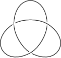
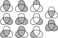
Figure 3. A trefoil knot diagram and its alternated cycles.

Definition 2.2.

The resistance energy (or RE for short) is

$$RE(\gamma)=\sum\limits_{\ell\in\operatorname{Alt}(\gamma)}\frac{1}{A(\ell)}.$$

There is a serious practical disadvantage in using resistance energy. The number of cycles in the diagram grows very rapidly with respect to the crossing number; in the next two subsections we show how to fix this problem.

Let us illustrate the situation with the following example. Consider a graph $G(n)$ isomorphic to the $n\times n$ lattice as on Figure 3 (left).

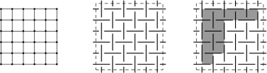
Figure 4. The graph $G(5)$, the corresponding alternated diagram $G^{*}(5)$, and an alternated cycle representing a Young diagram of shape $(5,2,2,2,1)$.

The number of cycles in $G(n)$ grows very rapidly with respect to $n$:

G(n)	$n=1$	$n=2$	$n=3$	$n=4$	$n=5$
Number of vertices	4	9	16	25	36
Cycles in $G$	1	13	213	9349	1222363

Suppose our diagram contains an alternated region $G^{*}(n)$ whose graph is homeomorphic to $G(n)$ as on Figure 3 (center).

Remark 2.3.

A region like $G^{*}(n)$ often occurs in a slightly perturbed $\infty$-shaped curve passed several times in the neighborhood of a former point of self-intersection.

Now we choose alternated cycles of $G^{*}(n)$ among all the cycles of $G(n)$. Let us give a general estimate. The region $G$ has $(n+1)^{2}$ double points. For the number of cycles and alternated cycles in $G(n)$ and in $G^{*}(n)$, respectively, we have the following lower bounds.

Proposition 2.4.

The number of cycles in $G(n)$ is at least

$$\frac{4^{n}(n+1)}{\sqrt{\pi}n^{3/2}}-1.$$

The number of alternated cycles in $G^{*}(n)$ is at least

$$\frac{2^{n}}{\sqrt{2\pi n}}-1.$$

Proof.

The number of nonempty disks in the shape of Young diagrams in $G(n)$ (see an example in Figure 3 (right) is exactly ${2n\choose n}-1$. The boundaries of these disks are cycles. A simple estimate shows that at least ${n\choose\lfloor n/2\rfloor}-1$ of the corresponding cycles in $G^{*}(n)$ are alternated. The asymptotics for Catalan numbers is

$$C_{n}\approx\frac{4^{n}}{\sqrt{\pi}n^{3/2}}.$$

This implies the estimates of the proposition. ∎

Corollary 2.5.

The asymptotical growth of the maximal number of alternated cycles of diagrams with $N$ double points is at least $C\frac{2^{n/2}}{\sqrt{n}}$ for some constant $C$.

In fact, the real growth should be even higher. From the computational point of view, such a growth rate is not acceptable. In the next subsections, we describe two ways of reducing the running time.

We conclude this subsection with an interesting geometric probabilistic problem that arises here. Denote by $D_{m}$ be a two-dimensional disk with $m$ holes. Consider a graph $G\subset\mathbb{R}^{2}$. Denote by $\#(G,D_{m})$ the number of closed subsets of $\mathbb{R}^{2}$ homeomorphic to $D_{m}$ with boundary in $G$. Note that the number of cycles in a planar graph coincides with $\#(G,D_{0})$. The natural problem here is to find the distributions of such numbers with respect to the crossing number of $G$. In addition, we have the following particular asymptotic problem for $G(n)$.

Problem 2.

For nonnegative integers $m_{1}$ and $m_{2}$ find the following limit

$$\lim\limits_{n\to\infty}\frac{\#(G(n),D_{m_{1}})}{\#(G(n),D_{m_{2}})}.$$

2.2. Material resistance energy

Consider a knot made of wire lying on the plane. If the area of alternated cycles is large enough, then no resistance arises when we move the wire. Resistance arises only when the area of some alternated cycle is comparable with the width of the wire. We formalize this in the following definition. A cycle is called $\delta$-critical if its area is less than $\delta$. Denote the set of all alternated $\delta$-critical cycles of a diagram $\gamma$ by $\operatorname{Alt}_{\delta}(\gamma)$.

Definition 2.6.

The material resistance energy (or $MRE_{\delta}$ for short) is

$$MRE_{\delta}(\gamma)=\sum\limits_{\gamma\in\operatorname{Alt}_{\delta}(\gamma)}\left(\frac{1}{A(\gamma)}-\frac{1}{\delta}\right).$$

In general, the parameter $\delta$ depends on the shape (width, i.e., on $\varepsilon$) of the wire. In the situation of ideal wire (of zero width, i.e., when $\delta$ tends to 0), the support of the functional $MRE_{0}$ is contained in the set of all singular knot diagrams.

The main advantage in this approach is that generically there are not too many alternated cycles whose areas are very small (basically tending to 0), so the majority of cycles are not in $\operatorname{Alt}_{\delta}(\gamma)$. One may determine the set $\operatorname{Alt}_{\delta}(\gamma)$ in the following two steps.

Step 1. Find the “low-area” domains containing all simple cycles for which the area is less than $\delta$ (we say that a cycle is simple if it does not contain other points of the diagram in the interior).

Step 2. For each connected component of each low-area domain, check all the alternated cycles contained in its closure.

Remark 2.7.

The MRE-functional simulates the real situation with a thin wire, for which it is impossible to have infinitely many cycles in diagrams, hence in real life the value of the MRE-functional is always finite. Anyway, the corresponding algorithms usually work with a piecewise discretization of knots, and for polygonal knots the amount of cycles is always finite.

2.3. Genericity modification of MRE

The MRE-functional still has a disadvantage: small-area regions like $G^{*}(n)$ may occur at some moment of the gradient flow. This will lead to an enormous increase in the complexity of the gradient calculation. In this subsection, we modify the MRE-functional in such a way that one needs to study only loops, 2-gonal, triangular, and quadrangular cycles.

Denote by $\operatorname{Crit}_{\delta}^{4}(\gamma)$ the set of all 4-arc cycles in $\gamma$, denote also by $\operatorname{Alt}_{\delta}^{\leq 3}(\gamma)$ the set of all alternated loops, 2-, and 3-cycles. Let

$$\Gamma_{\delta}(\gamma)=\operatorname{Alt}_{\delta}^{\leq 3}(\gamma)\cup\operatorname{Crit}_{\delta}^{4}(\gamma).$$

Definition 2.8.

The genericity material resistance energy (or $GMRE_{\delta}$ for short) is

$$GMRE_{\delta}(\gamma)=\sum\limits_{\ell\in\Gamma_{\delta}(\gamma)}\left(\frac{1}{A(\ell)}-\frac{1}{\delta}\right).$$

Any diagram with $n$ crossings has less then ${n^{p}}/{p!}$ cycles with $p$ arcs each. Hence the amount of cycles in $\Gamma_{\delta}(D)$ is always bounded by

$$\frac{n^{4}}{24}+\frac{n^{3}}{6}+\frac{n^{2}}{2}+n.$$

2.4. On the deformation of knot diagrams

Let $\gamma:S^{1}\to\mathbb{R}^{2}$ be a $C^{2}$-regular curve. We say that $\gamma$ is immersed if the image $\gamma(S^{1})$ has finitely many double points of transversal self-intersections. We say that $\gamma$ is codimension-one-immersed if it has finitely many double points of transversal self-intersections and either a triple point of transversal self-intersection or a double point at which the intersection is not transversal.

Let $\gamma_{t}$ be a deformation in the space of regular curves of $S^{1}$ into $\mathbb{R}^{2}$. We say that a deformation $g_{t}$ is generic if for all but a finite number of points $t$ the image $g_{t}(S^{1})$ is immersed, and at these points it is codimension-one-immersed.

We consider a knot diagram as an immersed curve equipped with a crossing type (i.e., overpass-underpass information) at each double point. We also extend the notion of knot diagram to the case of codimension-one-immersed curves. From computational point of view it is worthy to preserve the crossings (at least locally for triple points). So we regard a triple point as three double points and specify crossing types at all these double points (without taking care whether such three crossings are realizable as the projection of a knot or not). A tangential double point is regarded as a pair of double points of the same crossing type. Denote the space of all immersed and codimension-one-immersed diagrams by $\mathcal{D}$.

A deformation $\gamma_{t}$ in $\mathcal{D}$ is generic if for all but a finite number of points $t$ the image $g_{t}(S^{1})$ is immersed, at these points it is codimension-one-immersed, and the crossing types depend smoothly on the crossings with respect to the parameter $t$.

Remark 2.9.

Notice that a generic deformation of a diagram (in our definition) does not necessarily preserve the knot type. It can change while passing through a codimension-one-regular diagram with a triple point, like it does on the following picture.

Theorem 2.10.

Let $\gamma_{t}$ be a generic deformation in the space of regular knot diagrams with parameter $t$ in $[0,1]$. Suppose that there exists $\delta$ such that the $GMRE_{\delta}$-functional is uniformly bounded from above for the whole deformation. Then the knot types of $\gamma_{0}$ and of $\gamma_{1}$ coincide.

Proof.

Since the deformation is generic, the diagrams occurring in the deformation have only double tangency points or triple points. The surgeries at these points are described by the second and the third Reidemeister moves. All other surgeries are forbidden, otherwise an alternated cycle disappears (but its area is bounded from below by $1/C$). ∎

2.5. Total energy related to the pendulum

Let us say a few words about the combination (sum) of the uniformization functional $U_{f}$ for $f(x)=x^{2}$ and the material resistance energy $MRE$, i.e.,

$$E(\gamma)=U_{x^{2}}(\gamma)+MRE_{\delta}(\gamma).$$

Critical positions of $U_{x^{2}}$ are either circles passed several times or $\infty$-shaped curves passed several times. In the case of a nonzero Whitney index, the functional $MRE_{\delta}$ does not allow the knot diagram to reach the shape of perfect circles or perfect $\infty$-shaped curves. The knot diagram ends up either as a circular braid (which is almost a circle passed several times) or as almost an $\infty$-shaped curve passed several times. In addition, it is possible that the gradient flow will take the knot diagram to a diagram containing alternated cycles of small area. For instance, this is the case when the knot type is non-trivial and the Whitney index of the starting curve is one. So we have the following

Theorem 2.11.

The critical knots for the energy

$$E(\gamma)=MRE_{\delta}(\gamma)+U_{x^{2}}(\gamma)$$

are either a circle passed once, or an $\infty$-shaped curve passed once, or contains at least one alternated cycle of area less than $\delta$.

Proof.

In Theorem 1.7, we showed that the critical curves for $U_{x^{2}}$ are exactly circles and $\infty$-shaped curves. For all other critical points, the functional $MRE_{\delta}$ must contribute, which implies that at least one of the critical cycles is of area less then $\delta$. ∎

The same statement holds for the repulsive energy $GMRE_{\delta}$.

Theorem 2.12.

The critical knots for the energy

$$E(\gamma)=GMRE_{\delta}(\gamma)+U_{x^{2}}(\gamma)$$

are either a circle passed once, or an $\infty$-shaped curve passed once, or contains at least one alternated cycle of area less than $\delta$. ∎

3. Perspectives

In the sequel to this paper, we intend to describe the results of computer experiments with the functionals defined above, or, more precisely, with discretizations of these functionals. We conjecture that the experiments will show that the normal forms obtained classify flat $\varepsilon$-knots up to flat isotopy, but only when the number $c$ of crossings is small (say $c\leq 30$).

A further potentially interesting direction of study is related to the application of Theorem 1 from [12], which asserts that there is a deep relationship between normal forms of flat $\varepsilon$-knots and those of ordinary (3D) knots, in order to obtain information on the latter by using results obtained for the former.

References

- [1] S. Bryson, M. H. Freedman, Z.-X. He, and Z. Wang, Möbius invariance of knot energy, Bull. Amer. Math. Soc. (N.S.), vol. 28 (1993), no. 1, pp. 99–103.
- [2] M. H. Freedman, Z.-X. He, Links of tori and the energy of incompressible flows, Topology vol. 30 (1991), no. 2, pp. 283–287.
- [3] M. H. Freedman, Z.-X. He, and Z. Wang, Möbius energy of knots and unknots, Ann. of Math. (2), vol. 139 (1994), no. 1, pp. 1–50.
- [4] W. Fukuhara, Energy of a knot, The fête of topology, Academic Press, (1988), pp 443–451.
- [5] O. Karpenkov, Energy of a knot: variational principles Russian J. of Math. Phys. vol. 9(2002), no. 3, pp. 275–287.
- [6] O. Karpenkov, Energy of a knot: some new aspects Fundamental Mathematics Today, Nezavis. Mosk. Univ., Moscow (2003), pp. 214–223.
- [7] O. Karpenkov, The Möbius energy of graphs, Math. Notes, vol. 79(2006), no. 1-2, pp. 134–138.
- [8] D. Kim, R. Kusner, Torus Knots Extremizing the Möbius Energy, Experimental Mathematics, vol. 2(1993), no. 1, pp. 1–9.
- [9] H. K. Moffat, The degree of knottedness of tangled vortex lines, J. Fluid Mech. vol. 35 (1969), 117–129. pp. 29–76.
- [10] J. O’Hara, Energy of a knot, Topology, vol. 30(1991), no. 2, pp. 241–247.
- [11] J. O’Hara, Family of energy functionals of knots, Topology Appl. vol 48(1992), no. 2, pp. 147–161.
- [12] J. O’Hara, Energy functionals of knots II, Topology Appl. vol. 56(1994), no. 1, pp. 45–61.
- [13] J. O’Hara, Energy of Knots and Conformal Geometry, K & E Series on Knots and Everything – Vol. 33, World Scientific, 2003, 288 p.
- [14] A. B. Sossinsky, Mechanical Normal Forms of Knots and Flat Knots, Russ. J. Math. Phys. vol. 18, no. 2 (2011).