On radial geodesic forcing of zonal modes

Abstract

The elementary local and global influence of geodesic field line curvature on radial dispersion of zonal modes in magnetised plasmas is analysed with a primitive drift wave turbulence model. A net radial geodesic forcing of zonal flows and geodesic acoustic modes can not be expected in any closed toroidal magnetic confinement configuration, since the flux surface average of geodesic curvature identically vanishes. Radial motion of poloidally elongated zonal jets may occur in the presence of geodesic acoustic mode activity. Phenomenologically a radial propagation of zonal modes shows some characteristics of a classical analogon to second sound in quantum condensates.

I Introduction

Zonal modes play an important role in turbulent self organisation of quasi two-dimensional fluids, such as magnetised plasmas or in geophysical, planetary and stellar fluid dynamics Diamond05 ; Fujisawa09 ; Manz09 . Zonal flows can be regarded as a low-frequency spectral condensate phase of the turbulence Hallatschek00 ; Shats05 featuring the highest flow symmetry allowed by the (generically inhomogeneous) system: atmospherical and oceanic zonal jets are latitudinally extended flow structures, and zonal modes in toroidal fusion plasmas appear as average flows on magnetic flux surfaces.

Geophysical zonal flows can experience temporal variations and oscillations caused by seasonal or topographical influences, and may migrate meridionally. Similarly, plasma zonal flows in the inhomogeneous toroidal magnetic field are modulated by finite frequency geodesic acoustic mode (GAM) oscillations Winsor68 . The possibility of radial propagation of zonal flows and GAMs in fusion plasmas has recently attracted interest, motivated by indicating experimental observations Ido06 ; Lan08 ; Liu10 .

Previous studies on radial propagation included analytical theory of GAMs and zonal flows Smolyakov00 ; Gao08 ; Miki10 and linear simulations of GAMs Sasaki08 ; Xu08 ; Xu09 . Finite Larmor radius (FLR) effects in the presence of a background temperature gradient have been identified as one potential mechanism for radial propagation of zonal modes Itoh06 ; Zonca08 ; Sasaki08 ; Xu08 ; Xu09 . Further, it had been postulated that details of the magnetic field geometry, in particular an up-down asymmetry, could cause radial GAM migration Hager09 ; Hager10 .

In the following the particular influence of geodesic curvature and up-down asymmetry on the radial dispersion of zonal modes is analysed. A basic geometric property has to be recollected in this context: the flux surface (zonal) average of geodesic curvature is zero in any toroidal configuration. Real and artificial geodesic forcing effects on zonal modes are discussed, including the perils of using inadequately simple geometry models that violate this property.

The computational analysis shall here be based on a self-consistent nonlinear model including both the drift wave turbulence fluctuation component and the zonal mode condensate. Radial propagation can best be studied when radial boundary conditions are eliminated by using a periodic domain. This however excludes the utilization of 3-D flux-tube models, which rely on finite magnetic shear to avoid unphysical flute modes but thereby introduce radial secularity.

The most primitive model for self-sustained drift wave turbulence in magnetised plasmas, that also allows radially periodic boundary conditions, is the two-dimensional Hasegawa-Wakatani (HW) set of equations Hasegawa83 . This standard model is here extended to specifically study geodesic curvature effects.

The paper is organised as follows: in section II the curvature modifications to the HW model are introduced. The linear local radial dispersion relation of geodesically forced zonal HW modes is discussed in section III. Numerical details regarding the nonlinear simulations are presented in Chapter IV. Computational results on local geodesic forcing of turbulence generated zonal flows are reported in section V. The essential flux-surface property of zero average geodesic curvature and pitfalls concerning simplified geometry models are reviewed in section VI: violation of this constraint results in unphysical radial propagation of zonal flows and GAMs. Poloidal variation of curvature is introduced in section VII, and effects on apparent radial propagation of zonal modes is discussed in section VIII. Finally, in section IX, a striking analogy to the phenomenon of “second sound” in quantum condensates is presented.

II Turbulence-flow model

First, consider the HW model for drift wave turbulence Hasegawa83 . It accounts for nonlinear instability driven by a gradient $\nabla n_{0}(x)$ in plasma density and resistive parallel coupling between fluctuations of density $n$ and electrostatic potential $\phi$. The resulting turbulent state of $E\times B$ vortices in the $(x,y)$ drift plane perpendicular to the magnetic field can form low-frequency $k_{y}=0$ zonal flow structures with a finite wave number $k_{x}$. The HW model is in the following employed with modifications for zonal flow corrections on the dissipative coupling Dorland93 and including magnetic field line curvature terms Scott05NJP :

$$\partial_{t}\Omega+[\phi,\Omega] =d(\hat{\phi}-\hat{n})-\kappa(n),$$ (1)

$$\partial_{t}n+[\phi,n] =d(\hat{\phi}-\hat{n})-g_{n}\partial_{y}\phi+\kappa(\phi-n).$$ (2)

Standard drift normalisation is applied Scott05NJP . The electrostatic potential $\phi$ is obtained from the vorticity $\Omega$ by

$$\nabla^{2}\phi=\Omega.$$ (3)

In the dissipative coupling term the zonal ($y$) average is subtracted from density and potential fluctuations Dorland93 :

$$\hat{\phi}=\phi-\langle\phi\rangle,\qquad\hat{n}=n-\langle n\rangle.$$ (4)

In toroidal plasma geometry the $x$ coordinate locally represents the minor radial, and $y$ the poloidal direction.

The original HW model (with $\kappa=0$) is determined by the dissipative coupling parameter $d$ (proportional to $k_{||}^{2}$) and the density gradient scale length $g_{n}$. The hydrodynamic limit of the Euler equations is recovered for $d=0$ and $g_{n}=0$, while the adiabatic limit $d\gg 1$ asymptotically corresponds to the Hasegawa-Mima-Charney-Obukhov equation. The general properties of the HW model have been extensively discussed elsewhere (e.g. in Refs. Koniges92 ; Biskamp94 ; Pedersen96 ; Zeiler96 ; Hu97 ; Camargo98 ; Korsholm03 ; Priego05 ; Numata07 ; Tynan07 ).

The extended model here further includes field line curvature effects. Normal and geodesic components of the magnetic curvature ${\cal K}=\nabla\ln B$ enter the compressional effect on vortices due to magnetic field inhomogeneity by

$$\kappa=\kappa_{y}\partial_{y}+\kappa_{x}\partial_{x}$$ (5)

where the curvature components in toroidal geometry are a function of the poloidal angle $\theta$. For a circular torus $\kappa_{y}\equiv c_{B}\cos(\theta)$ and $\kappa_{x}\equiv c_{B}\sin(\theta)$ when $\theta=0$ is defined at the outboard midplane. Pure interchange drive is acting for $\theta=0$ and pure geodesic effects for $\theta=\pm\pi/2$, and mixed effects are achieved for intermediate angles. Slab turbulence is recovered for $c_{B}=0$.

In the following, at first the local influence of geodesic curvature on zonal modes in drift wave turbulence is discussed by choosing a constant angle $\theta$ for the whole $y$-domain. Later, a periodic dependence of the form $\theta(y)=2\pi(y-L_{y}/2)/L_{y}$ will be introduced to globally map the magnetic curvature inhomogeneities on a flux surface into the simulation domain.

III Linear analysis: local geodesic forcing of zonal modes

Fourier analysis with an ansatz $n,\phi\sim\exp(i{\bf k}\cdot{\bf x}+i\omega t)$ and linearisation of eqs. (1) and (2) for $k_{y}\ll k_{x}$ and $d=0$ (zonal modes) in the local approximation provides

$$\omega k_{x}^{2}\phi_{k} =\kappa_{x}k_{x}n_{k}$$ (6)

$$\omega n_{k} =\kappa_{x}k_{x}(\phi_{k}-n_{k})$$ (7)

For global simulations covering the whole flux surface (in an annulus or flux-tube representation) the averages $\langle\kappa_{x}n_{k}\rangle_{y}$ and $\langle\kappa_{x}\phi_{k}\rangle_{y}$ of the geodesic curvature operator acting on the fluctuations would have to be taken into account in the linear analysis (see section VII): sideband modes of the density then will result in the well-known geodesic acoustic oscillations at the GAM frequency.

In the present local discussion in this section, $\langle\kappa_{x}\rangle_{y}$ in itself is assumed to be nonzero and constant, and global sideband modes are neglected. This artificial scenario however can apply to zonal jet modes with nonzero but small $k_{y}\ll k_{x}$ (rather than zonal flows with exactly $k_{y}=0$), and it corresponds to artificial situations where a finite flux-surface average geodesic curvature results from an improper geometry model.

The resulting local zonal wave equation has a frequency

$$\omega=c_{x}k_{x}(\pi\pm\lambda)$$ (8)

which is nonzero for finite average geodesic curvature, where $c_{x}=-(\kappa_{x}/2\pi)$ and $\lambda=(\pi/k_{x})\sqrt{4+k_{x}^{2}}$. The finite $k_{x}$ zonal modes are actually nonlinearly driven by turbulent Reynolds stress, which is eliminated in the zonal dispersion relation eqs. (6) and (7) by linearisation.

The dispersion relation results in a phase velocity

$$v_{ph}={\omega\over k_{x}}=c_{x}(\pi\pm\lambda).$$ (9)

For $k_{x}\ll 1$ follows $\lambda\approx 2\pi/k_{x}$ so that $\omega\approx 2\pi c_{x}$ is asymptotically independent of the wave number. Radial modulation of zonal modes is in this long wavelength limit obtained by a local phase velocity

$$v_{ph}\approx c_{x}\lambda.$$ (10)

The group velocity $v_{gr}=\partial\omega/\partial k_{x}\approx\pi c_{x}$ is for $k_{x}\ll 1$ much smaller than the phase velocity. The following numerical simulations will show that zonal flows and GAMs mostly appear with one dominant radial mode number propagating with $v_{ph}$. For single modes the concept of a wave packet travelling with a group velocity is not relevant. Thus a Poynting approach on GAM propagation Hager09 is pointless.

In the following the simple analytical relation (10) is numerically tested locally, and the effect of an artificial non-zero average geodesic curvature $c_{x}$ on radial propagation of zonal modes is demonstrated and visualized.

IV Nonlinear numerical solution

Equations (1) and (2) are numerically solved in time with an explicit 3rd order Karniadakis scheme Karniadakis , and the Poisson brackets $[a,b]=(\partial_{x}a)(\partial_{y}b)-(\partial_{y}a)(\partial_{x}b)$ are evaluated with the energy and enstrophy conserving Arakawa method Arakawa . The numerical method is equivalent to the one in Refs. Naulin03 ; Scott05NJP ; Numata07 . Hyperviscuous operators $\nu^{4}\nabla^{4}$, with $\nu^{4}=-2\cdot 10^{-4}$, are added for numerical stability to the right hand side of both equations (1) and (2), acting on $\Omega$ and $n$, respectively.

Eq. (3) is for a double periodic domain efficiently solved in $k$ space by evaluation of $\phi_{k}=-\Omega_{k}/k_{\perp}^{2}$. Threaded FFTW3 libraries are employed for the 2-D forward and backward Fourier transforms FFTW3 . The use of openMP multi-threaded FFTW3 routines on an 8-core workstation turned out to be parallel efficient up to 4 threads only for the specified grid size due to overhead costs.

The equations are here discretised on a doubly periodic grid with various (in general not quadratic) box dimensions. Spatial scales are in units of the drift scale $\rho_{s}=\sqrt{T_{e}M_{i}}/(eB)$ where $T_{e}$ is the electron temperature, $M_{i}$ is the ion mass, and $B$ is the magnetic field strength. The gradient length scale $g_{n}=L_{\perp}/L_{n}\equiv 1$ is fixed by specifying $L_{\perp}=L_{n}=|\nabla\ln n_{o}|^{-1}$. This normalises the time scale to $t\rightarrow t\;c_{s}/L_{n}$. A stable time step for nominal parameters on a $512\times 512$ grid with $L_{x}=L_{y}=128\rho_{s}$ scale was found to be $\Delta t=0.0025$. The computations are initialized with a random bath of quasi-turbulent density fluctuations, run into a saturated turbulent state (typically obtained for $t>500$) and are continued for statistical analysis.

V Local results: radial propagation of zonal modes

The radial zonal flow structure with respect to local normal and geodesic curvature effects is in the following numerically analysed by varying the poloidal angle $\theta$ through different simulations, while $\theta$ takes a constant value on the respective ($x,y$) domains.

Nominal values for the dissipative coupling and curvature parameters used here are $d=0.5$ and $c_{B}=0.05$. The flows are dominantly zonal for these parameters, and are blocked for lower forcing ($d\lesssim 0.1$ and without interchange drive). The radial mode number $l$ of zonal flows increases with stronger forcing.

Radial wave number spectra $|\phi|(k_{x})$ for the $d=0.5$ flow dominated scenario are shown in Fig. 1: For the standard HW slab case ($c_{B}=0$, thin dashed line) the radial wave number features a distinct peak at $k_{x}\approx 0.39$ in units of $\rho_{s}$. This corresponds to an $l=8$ radial mode of the ($m=0$, $n=0$) zonal flow with radial wavelength $\lambda=2\pi/k_{x}\approx 16\rho_{s}$. Further contributions from $l=6$ and $l=10$ modes are an order of magnitude smaller. The mixed curvature case ($\theta=\pi/8$, bold line) shows a strong maximum for $l=10$ and a broader spectrum with similar amplitudes for $l=4$, 5, 7, and 8 modes.

Figure 1: Radial wave number $k_{x}$ (in units of the drift scale $\rho_{s}$) spectra of the potential $|\phi|^{2}$. Bold line: mixed curvature effect ($c_{B}=0.05$, $\theta=\pi/8$); thin dashed line: slab case ($c_{B}=0$).

(a)
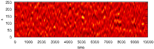
(b)
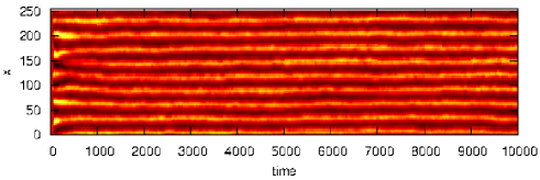
(c)
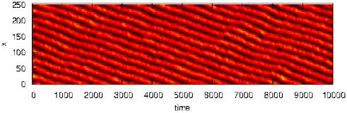
(d)
(e)

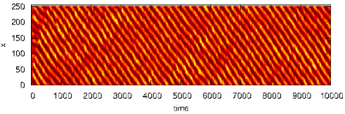
Figure 2: Zonal potential $\langle\phi\rangle(t,x)$ for various cases of forcing and curvature parameters:
(a) blocked flow for low forcing ($d=0.1$, $c_{B}=0$); (b) zonal flow for high forcing ($d=0.5$, $c_{B}=0.05$, $\theta=0$); (c) mixed curvature case ($d=0.5$, $c_{B}=0.05$, $\theta=\pi/8$); (d) same but reversed field ($d=0.5$, $c_{B}=0.05$, $\theta=-\pi/8$); (e) pure geodesic drive ($d=0.5$, $c_{B}=0.05$, $\theta=\pi/2$).

This radial structure of the zonal flow modes is also clearly visible in 2-D ($t$,$x$) plots for cases with strong forcing. Fig. 2 shows the time evolution of the zonally averaged potential for various drive parameters and poloidal angles. Here the spatial resolution is reduced to 256 $\times$ 256 grid points for the same physical domain size of $L_{y}=128\rho_{s}$ as before. Runs are now taken to $t=10^{4}$.

As predicted above, the zonal modes propagate radially with a velocity proportional to the geodesic curvature parameter $c_{x}$ and to the wavelength $\lambda=L_{x}/l$. The phase velocity measured in the nonlinear simulation is in very good agreement with the estimate obtained from linear theory. For case (e) with $c_{x}=-c_{B}/(2\pi)\approx-0.008$ and $\lambda/\rho_{s}=128/8=16$ we expect $v_{ph}\approx c_{x}\lambda\approx 0.064$ from equation (10), while the simulation gives $v_{sim}=\Delta x/\Delta t=128/1860\approx 0.069$.

At this point it should again be stressed that this local result as a test for eq. (10) does not apply to actual toroidal $k_{y}=0$ zonal flows. It will however be relevant for the following discussion on geometrical artefacts and on the interpretation of spatio-temporal features identified as radially propagating zonal jet structures.

VI Flux-surface property of geodesic curvature

In a torus the “upper” and “lower” regions locally correspond to positive and negative $c_{x}$, respectively, if the poloidal coordinate $\theta$ is chosen as here to be aligned “upwards”. Reversal of the magnetic field direction will locally also reverse the sign of the geodesic term through $c_{x}(-\theta)=-c_{x}(\theta)$. For a circular torus $\kappa_{x}=c_{B}\sin(\theta)$.

The poloidally local effects of radial geodesic forcing globally balance, if positive and negative contributions from geodesic curvature cancel by integration over a flux surface. This is indeed the case for any low beta toroidal MHD equilibrium, including up-down asymmetric tokamaks or 3-D stellarator configurations. The flux surface average of the geodesic curvature always identically vanishes Hazeltine85 .

This is illustrated in Fig. 3 (a) where the geodesic curvature $\kappa_{x}(\theta)$ as a function of the poloidal angle is shown for the example of a real up-down asymmetric ASDEX Upgrade equilibrium in a lower single-null configuration, calculated with the VMEC equilibrium code Strumberger at a radial position $\rho=V/V_{o}=0.95$ in volume coordinates. The maximum of geodesic curvature is reduced in the vicinity of the X-point location $\theta=+\pi/2$, but the average over $\theta$ remains zero as expected. This peak reduction affects the GAM and zonal flow amplitudes (and consequently turbulent transport) through the same mechanisms as by the up-down symmetric effect of flux-surface elongation Kendl03 ; Kendl05 ; Kendl06 .

In no toroidal configuration a net radial propagation of ($m=0$, $n=0$) zonal modes by geodesic forcing alone is therefore possible.

Approximate analytical toroidal geometry models (e.g. when introducing up-down asymmetry effects) have to account for this cancellation, otherwise unphysical radial propagation may appear in simulations. This is illustrated in Fig. 3 (b): here $\kappa_{x}(\theta)$ (bold line) has been calculated from the simple up-down asymmetric model geometry from Ref. Hager10 , where flux surfaces are vertically shifted. It can be clearly realised that this corresponds to a shift $\kappa_{x}(\theta)\approx c_{0}+c_{B}\sin\theta$ with the result of a nonzero average geodesic curvature. This unphysical finite average acts on GAMs and zonal flows exactly like the local model discussed in Sections III and IV and results in an artifical radial propagation. Other simplified analytical geometry models in general also do not conserve the zero average geodesic curvature property.

Most results concerning the overall turbulence and flow levels and other characteristics from nonlinear simulations are usually not or only to a very small degree affected by this particular inconsistency. Simple X-point models for example well allow to study an influence of local magnetic shearing on turbulence and transport. For any discussion of radial propagation of GAMs and zonal flows the use of analytical model geometries has to either explicitly account for a zero average or is otherwise inappropriate. Then numerical solutions from codes that solve actual MHD equilibria are required.

(a)
(b)

Figure 3: (a) Geodesic curvature $\kappa_{x}(\theta)$ in a circular torus (sinusoidal thin curve) and in a realistic ASDEX Upgrade equilibrium (bold curve). The average always is identically zero.
(b) Geodesic curvature $\kappa_{x}(\theta)$ resulting from an inappropriately simple X-point geometry model (bold curve), which leads to an unphysical finite average.

VII 2-D geodesic acoustic modes

Next, a poloidal variation of the geodesic curvature within the 2-D HW computational domain is taken into account. The extension $L_{y}$ is elongated up to $L_{y}/L_{x}=16$ in order to cover a complete poloidal circumference. The curvature terms $\kappa_{y}\equiv c_{B}\cos(\theta)$ and $\kappa_{x}\equiv c_{B}\sin(\theta)$ are now periodically varying along the $y$ coordinate by $\theta(y)=2\pi(y-L_{y}/2)/L_{y}$. The average along $y$ can so be interpreted as the flux surface average, while still any parallel (3-D) dynamics is neglected.

The linear spectral zonal HW equations now become

$$\omega k_{x}^{2}\langle\phi_{k}\rangle =\langle\kappa_{x}k_{x}n_{k}\rangle$$ (11)

$$\omega\langle n_{k}\rangle =\langle\kappa_{x}k_{x}(\phi_{k}-n_{k})\rangle$$ (12)

where the brackets denote the average along $y$. Using the identity $\sin^{2}\theta=1-\cos^{2}\theta={1\over 2}[1-\cos(2\theta)]$ and defining the zonal flow velocity by $u_{k}\equiv ik_{x}\langle\phi_{k}\rangle$, the dispersion relation gives $\omega^{2}u_{k}={1\over 2}c_{B}^{2}u_{k}$. The result is a periodic oscillation of the zonal flow with the GAM frequency $\omega=c_{B}/\sqrt{2}\equiv\omega_{GAM}$.

The present 2-D HW model lacks any parallel effects of field line connection and wave dynamics. In particular, the absence of coupling from the density sideband to parallel dissipative sound and Alfvén dynamics overestimates the GAM amplitude, compared to 3-D flux-tube simulations Scott02 . On the other hand, the density sideband is also in 2-D nonlinearly coupled to the density cascade and its respective small-scale dissipation. The geodesic transfer thus constitutes a sink mechanism for zonal flow energy, and the 2-D toroidal zonal flow amplitude is less than in the slab or local case (and also less than in 3-D toroidal simulations).

The results are clearly quantitatively different from more complete 3-D (drift-Alfvén or gyrofluid) models, but the emphasis here is on principle understanding of basic curvature coupling mechanisms which do not specifically rely on parallel dynamics.

VIII Spatiotemporal zonal flow pattern: apparent radial motion

The poloidally extended model for $\kappa=\kappa(y)$ is now solved numerically with simulation parameters $d=0.5$, $g_{n}=1$, $n_{x}=128$, $n_{y}=2048$, $L_{x}=32\rho_{s}$, $L_{y}=512\rho_{s}$, $\nu^{4}=-5\cdot 10^{-4}$, $\Delta t=10^{-4}$, and with a curvature parameter $c_{B}=0.5$. The zonal flow velocity $\langle v_{y}\rangle(x,t)$ is shown during the initial saturated phase of the computation ($100<t<900$) in Fig. 4.

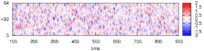
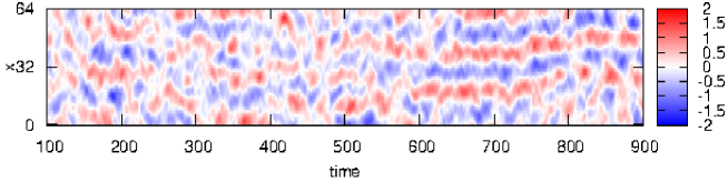
Figure 4: Pattern of zonal flow velocity $\langle v_{y}\rangle(x,t)$ for $c_{B}=0.5$ (top) and $c_{B}=0.25$ (bottom). Intermittent diagonal streaks bear semblance of radial “propagation” for high-frequency GAMs at $c_{B}=0.5$ but are absent for lower frequencies.

The plot for $c_{B}=0.5$ features an irregular checkerboard like pattern: quasi periodic oscillations appear both in space and time as the GAM modulation reverses the zonal flow. The radial wave number of the pattern is in the order $k_{x}\sim 1$ and the frequency in the order of $\omega\sim\omega_{GAM}$. When the curvature parameter is reduced to $c_{B}=0.25$ (with otherwise identical simulation parameters) the frequency scales proportionally but the modulation appears weaker and the zonal flow direction at a specific radial location $x$ rarely reverses with time.

Another feature of the pattern for $c_{B}=0.5$ immediately strikes the eye: some zonal flow structures appear connected diagonally and give the semblance of moving radially in time with a velocity $v_{x}^{app}=\omega/k_{x}$. The connections first appear randomly with no prefered radial direction. This in-out symmetry can be spontaneously broken and an effective diagonal pattern may emerge transiently (as can be seen for around $t\approx 100$ and $t\approx 500$). Occurrence and directionality of such symmetry breaking appear to be random and to depend on simulation parameters and resolution.

The resulting apparent radial motion however is illusionary as the actual spatio-temporal zonal checkerboard-like structures do not move. This appearence may mislead to the conclusion of GAMs propagating radially with $v_{x}^{app}\sim\omega_{GAM}/k_{x}$. But as it turns out it is not the GAM modulated zonal flows (or the GAMs) which are moving, but rather $k_{y}\ll 1$ vortices.

Vortex structures can be detected in a wide spatial range, from circular eddies in the size of $k_{y}\sim k_{x}\sim 1$ to $k_{y}=0$ zonal flows. In an intermediate range poloidally elongated vortices with $k_{y}\ll 1$ are visible. These “zonal jet” structures appear strained out by the zonal flow shear, like shown in Fig. 5.

Zonal jets are, in contrast to $k_{y}=0$ zonal flows, susceptible to geodesic forcing. The poloidally elongated structures can experience local forcing in the radial direction. Diagonal connections in the $\langle v_{y}\rangle(x,t)$ spatiotemporal GAM pattern appear through local radial zonal jet migration if the life time of the jets is comparable to the GAM period. For lower $c_{B}$ (e.g. 0.1) the vortex turnover period is much smaller than the GAM modulation time of the zonal flows, and no diagonal motion is observed in spatiotemporal diagrams.

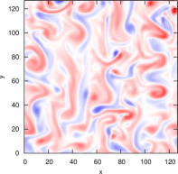
Figure 5: “Zonal jets”: $k_{y}\ll 1$ vortices strained out by zonal flow shearing (in particular around $x\approx 50$). Vorticity $\Omega(x,y)$ is shown (negative values: blue; positive values: red; in arbitrary units) on a part of the computational domain.

Up-down asymmetry will not change the average effect of geodesic forcing on ($k_{y}\equiv 0$) zonal flows and GAMs. It may however have an indirect effect on poloidally localized ($k_{y}\ll 1$) zonal jets. Asymmetric shaping also influences local magnetic shear, which is, for example, strongly enhanced near a (lower) single-null X-point Kendl03 . Zonal jets emerging through straining of drift wave vortices can be weaker at the (downward) poloidal location of strong magnetic shear, and may experience less geodesic forcing than on the other (up) side. Under such circumstances an effective geodesic forcing of zonal jets might actually appear. In order to consistently account for local magnetic shear effects in interplay with zonal flow shearing a 3-D (flux-tube) model is indispensible. This case is therefore not further considered within the simplified 2-D model of the present discussion.

It has been demonstrated in the preceeding sections that unphysical radial propagation of zonal flows and GAMs by geodesic forcing may apparently occur for certain computational set-ups. Radial propagation of zonal modes by other possible causes (for example by inhomogeneous FLR effects) is not disputed here.

IX “Second sound” in drift wave turbulence

Radially propagating zonal modes, however they may originate, bear a striking resemblence to the phenomenon of “second sound” in quantum codensates. Second sound in two-fluid systems, for example in superfluid He, describes the transport of temperature and entropy in the form of waves rather than by diffusion Enz74 ; Joseph89 . Phonons (“first sound”) are modulated by temperature waves (“second sound”), while the normal component and the condensate oscillate out of phase.

Drift wave turbulence can be considered within the framework of wave kinetics Diamond-Book . Wave density and temperature in this context do not refer to the fluid moments of the plasma particles, but rather to the population density and wave energy of the drift mode excitations.

The spectral drift wave mode density of the turbulence at a specific radial location is modulated in time by the passing wave of the radially propagating zonal flow condensate. Although the condensate phase does not by itself participate in radial plasma transport this leads to a radial wave like transfer of spectral mode energy, when the turbulent phase is co-existing with the propagating condensate. Phenomenologically this propagation shows characteristics of a classical analogon to second sound in quantum condensates: in a wave kinetic picture a mode temperature of the turbulent phase may be defined by the mean spectral energy, which is modulated by zonal condensate mode propagation in the form of a radial wave rather than by diffusive spreading.

The source of drift wave turbulence is, with respect to its two-dimensional character and dual cascade property, located within the spectral distribution around $k_{\perp}\rho_{s}\sim 1$ and is for many cases well separated from both dissipation and modulation (condensate) scales. Weakly damped second sound in drift wave turbulence of this form appears possible, in contrast to general 3-D turbulent Kolmogorov type systems Falkovich90 . A future more rigorous theoretical consideration of this phenomenon surely is eligible.

X Conclusions

Basic mechanisms of local and global radial geodesic forcing on zonal modes have been discussed with the 2-D HW standard model of drift wave turbulence. The main results are summarized as follows:

• Radial propagation of $k_{y}\ll 1$ zonal modes can occur by local geodesic forcing, which has been demonstrated by poloidally local simulations.

• A net radial geodesic forcing of $k_{y}=0$ zonal modes (zonal flows and GAMs) can not be expected in any closed toroidal magnetic confinement configuration, as the flux surface average of geodesic curvature always identically vanishes.

• Unphysical radial propagation of zonal flows and GAMs may appear in simulations that use inappropriately simple geometry models violating this zero average property.

• Apparent radial motion of spatio-temporal zonal mode patterns may be visually diagnosed in the presence of geodesic acoustic oscillations.

• Zonal jets with $k_{y}\ll 1$ occur as vortices strained out by $k_{y}=0$ zonal flows or GAMs and may experience local geodesic forcing.

• Radially migrating poloidally localized zonal jets lead to a diagonal connection in spatio-temporal GAM patterns, and in conclusion to an illusion of radial GAM propagation.

• Up-down asymmetry does not alter the average geodesic curvature from zero, and therefore does not affect radial geodesic forcing of zonal flows and GAMs.

• Up-down asymmetry may influence the local amplitude of zonal jets through local magnetic shearing.

• Phenomenologically a radial propagation of zonal modes shows some characteristics of a classical analogon to second sound in quantum condensates.

While the applicability of the 2-D HW model on realistic fusion plasmas is definitely limited, it has served to elucidate basic physical effects of the magnetic field geometry on drift wave turbulence and zonal flows. Any future computational studies with more complete models on radial propagation of zonal modes should not rely on inappropriately simplified geometry models but have to make use of actual MHD equilibria.

References

- (1) P.H. Diamond, S.-I. Itoh, K. Itoh, T.S. Hahm, Plasma Phys. Control. Fusion 47, R35 (2005).
- (2) A. Fujisawa, Nucl. Fusion 49, 013001 (2009).
- (3) P. Manz, M. Ramisch, U. Stroth Phys. Rev. Lett. 103, 165004 (2009).
- (4) K. Hallatschek, Phys. Rev. Lett. 84, 5145 (2000).
- (5) M.G. Shats, X. Xia, H. Punzmann, Phys. Rev. E 71, 046409 (2005).
- (6) N. Winsor, J.L. Johnson, J.J. Dawson, Phys. Fluids 11 2248 (1968).
- (7) T, Ido, Y. Miura, K, Hoshino, et al. Nucl. Fusion 46, 512 (2006).
- (8) T. Lan, A.D. Liu, C.X. Yu, et al. Phys. Plasmas 15 056105 (2008).
- (9) A.D. Liu, T. Lan, C.X. Yu, et al. Plasma Phys. Control. Fusion 52, 085004 (2010).
- (10) A.I. Smolyakov, P.H. Diamond, M. Malkov, Phys. Rev. Lett. 84, 491 (2000).
- (11) Z. Gao, K. Itoh, H. Sanuki, J.Q. Dong, Phys. Plasmas 15, 072511 (2008).
- (12) K. Miki and P.H. Diamond, Phys. Plasmas 17 032309 (2010).
- (13) M. Sasaki, K. Itoh, A. Ejiri, Y. Takase, Contrib. Plasma Phys. 48 68 (2008).
- (14) X.Q. Xu, Z. Xiong, Z. Gao, W.M. Nevins, G.R. McKee, Phys. Rev. Lett. 100, 215001 (2008).
- (15) X.Q. Xu, E. Belli, K. Bodi, et al. Nucl. Fusion 49 065023 (2009).
- (16) K. Itoh, S.-I. Itoh, P.H. Diamond, et al. Plasma Fusion Res. 1 037 (2006).
- (17) F. Zonca and L. Chen, European Physics Letters 83, 35001 (2008).
- (18) R. Hager, K. Hallatschek, Phys. Plasmas 16, 072503 (2009).
- (19) R. Hager, K. Hallatschek, Phys. Plasmas 17, 032112 (2010).
- (20) A. Hasegawa, M. Wakatani, Phys. Rev. Lett. 50, 682 (1983).
- (21) B.D. Scott, Plasma Phys. Control. Fusion 49, S25 (2007).
- (22) W. Dorland, G. Hammett, Phys. Fluids B 5, 812 (1993),
- (23) B.D. Scott, New J. Phys. 7, 92 (2005).
- (24) A.E. Koniges, J.A. Crotinger, P.H, Diamond, Phys. Fluids B 4, 2785 (1992),
- (25) D. Biskamp, S.J. Camargo, B.D. Scott, Phys. Lett. A 186, 239 (1994).
- (26) S.J. Camargo, D. Biskamp, B.D. Scott, Phys. Plasmas 2, 48 (1995)
- (27) T.S. Pedersen, P.K. Michelsen, J.J. Rasmussen, Phys. Plasmas 3, 2939 (1996).
- (28) A. Zeiler, D. Biskamp, J.F. Drake, Phys. Plasmas 3, 3947 (1996).
- (29) G.Z. Hu, J.A. Krommes, J.C. Bowman, Phys. Plasmas 4, 2116 (1997).
- (30) S.B. Korsholm, P.K. Michelsen PK, V. Naulin, Phys. Plasmas 6, 2401 (1999).
- (31) M. Priego, O.E. Garcia, V. Naulin, J.J. Rasmussen, Phys. Plasmas 12, 062312 (2005).
- (32) R. Numata, R. Ball, R.L. Dewar, Phys. Plasmas 14, 102312 (2007).
- (33) C. Holland, G. Tynan, J. James, et al. Plasma Phys. Control. Fusion 49, A109 (2007).
- (34) R.D. Hazeltine, J.D. Meiss, Phys. Rep. 121, 1-164 (1985).
- (35) Unpublished data, courtesy of E. Strumberger, IPP Garching.
- (36) A. Kendl, B.D. Scott, Phys. Rev. Lett. 90, 035006 (2003).
- (37) A. Kendl, B.D. Scott, Phys. Plasmas 12, 064506 (2005).
- (38) A. Kendl, B.D. Scott, Phys. Plasmas 13, 012504 (2006).
- (39) G.E. Karniadakis, M. Israeli, S.A. Orszag, J. Comput. Phys. 97, 414 (1991).
- (40) A. Arakawa, J. Comput. Phys. 1, 119 (1966).
- (41) V. Naulin, A. Nielsen, SIAM J. Sci Comput. 25, 104 (2003).
- (42) M. Frigo, S.G. Johnson, Proc. IEEE 93 (2), 216 (2005).
- (43) B.D. Scott, New Journal of Physics 4, 52 (2002).
- (44) C.P. Enz, Rev. Mod. Phys. 46, 705 (1974).
- (45) D.D. Joseph, L. Preziosi, Rev. Mod. Phys. 61, 41 (1989).
- (46) P.H. Diamond, S.I. Itoh, K. Itoh, Modern Plasma Physics, Vol. 1. Cambridge University Press, New York 2010.
- (47) G.E. Fal’kovich, Sov. Phys. JETP 70, 1042 (1990).