Variance squeezing and entanglement of the $XX$ central spin model

Abstract

In this paper, we study the quantum properties for a system that consists of a central atom interacting with surrounding spins through the Heisenberg $XX$ couplings of equal strength. Employing the Heisenberg equations of motion we manage to derive an exact solution for the dynamical operators. We consider that the central atom and its surroundings are initially prepared in the excited state and in the coherent spin state, respectively. For this system, we investigate the evolution of variance squeezing and entanglement. The nonclassical effects have been remarked in the behavior of all components of the system. The atomic variance can exhibit revival collapse phenomenon based on the value of the detuning parameter.

I Introduction

Quantum optics is based on the three fundamental processes, namely, field-field interaction, atom-field interaction and atom-atom interaction. The literature is quite rich by models representing these processes. Recently, the interest in the atom-atom (, i.e., spin-spin) interactions is growing up as it is a promising candidate in implementing the quantum computer. In this respect, we can find that the demonstration of the spin dynamics in the semiconductor structures has been remarkably increased in the last few years in connection with the new emerging areas of quantum computation and information bayat . There are various forms of the spin-spin systems such as XX model lieb , XY model jin and XXZ model chiara .

Spin models like Heisenberg spin chains or spin star systems, describing for example a single electron spin in a semiconductor quantum dot interacting with surrounding nuclear spins via hyperfine coupling mechanisms, have been extensively studied pratt . These models have been proved to be promising candidates for the generation and the control of assigned quantum correlations verstraete . Additionally, the central spin models can provide an appropriate description of quantum information processes such as the quantum state transfer [7] and the quantum cloning [8] . The Hamiltonian of the $XX$ central spin model that is composed by a localized spin, hereafter called central spin, coupled to $N$ spins with the same coupling constant $\lambda$, takes the form imamog ; Privman ; molmer ; gaudin ; molmeru :

$$\hat{H}=\frac{\Omega}{2}\hat{S}_{z}+\frac{\mu}{2}\sum\limits_{j=1}^{N}\hat{\sigma}^{j}_{z}+\lambda\sum\limits_{j=1}^{N}(\hat{S}_{+}\hat{\sigma}^{j}_{-}+\hat{S}_{-}\hat{\sigma}^{j}_{+}),$$ (1)

where $\hat{S}_{i}$ and $\hat{\sigma}^{j}_{i}(i=z,+,-)$ are the Pauli operators referring to the central spin and the surrounding spins, respectively; $\Omega$ and $\mu$ are the frequencies of the central spin and the surrounding ones, where we assume that all the surrounding spins have the same frequency. The architecture is analogous to the star distribution networks used in communications. Furthermore, this model is useful for sharing entanglement between different spins molmeru . In terms of the collective operators, which describes the $N$ spins, the above Hamiltonian can be expressed as physica1 ; physica2 ; physica3 ; physica4 ; physr4 :

$$\frac{\hat{H}}{\hslash}=\frac{\Omega}{2}\hat{S}_{z}+\mu\hat{J}_{z}+\lambda\left(\hat{J}_{+}\hat{S}_{-}+\hat{J}_{-}\hat{S}_{+}\right),$$ (2)

where $\hat{J}_{z}=\frac{1}{2}\sum\limits_{j=1}^{N}\hat{\sigma}^{j}_{z}$ and $\hat{J}_{\pm}=\sum\limits_{j=1}^{N}\hat{\sigma}^{j}_{\pm}$. These operators satisfy the following commutation rules:

$$\left[\hat{J}_{+},\hat{J}_{-}\right]=2\hat{J}_{z},\qquad\text{and}\qquad\left[\hat{J}_{z},\hat{J}_{\pm}\right]=\pm\hat{J}_{\pm}.$$ (3)

The Hamiltonian (1) has been frequently used in many physical systems like quantum dots imamog , two-dimensional electron gases Privman and optical lattices molmer . Additionally, it represents a realization of the so-called Gaudin model whose diagonalization has been derived via the Bethe ansatz in gaudin . This model has been frequently studied by Messina and his coworkers physica1 ; physica2 ; physica3 ; physica4 . The main objectives were to find the solution of the Schrodinger’s equation or to study the entanglement in the two-spin star system. In physica1 ; physica2 ; physica3 ; physica4 ; physr4 the authors have considered the central star spin is the object and its surroundings is the finite reservoir. Motivated by the importance of this system in the literature we devote this paper for demonstrating the quantum properties of the central spin and its surroundings. Precisely, we investigate the variance squeezing and the entanglement. Related to the entanglement, we study the entanglement between the central spin and the surroundings as well as among the spins of the surroundings. For the former we use the linear entropy, while for the latter we adopt the concept of spin squeezing. From the analysis we show that the nonclassical effects are noticeable in the behavior of all components of the system for certain values of the interaction parameters. We proceed, for reason will be clear in the following section we recast the Hamiltonian (2) in the following form:

$$\frac{\hat{H}}{\hslash}=\frac{\mu}{2}\hat{N}+\hat{C},$$ (4)

where

$$\hat{N}=\hat{J}_{z}+\frac{1}{2}\hat{S}_{z},\quad\hat{C}=\frac{\Delta}{2}\hat{S}_{z}+\lambda\left(\hat{J}_{+}\hat{S}_{-}+\hat{J}_{-}\hat{S}_{+}\right),\qquad\Delta=\Omega-\frac{\mu}{2}.$$ (5)

It is easy to prove that $\hat{N}$ and $\hat{C}$ are constants of motion.

This paper is prepared in the following order. In section II we derive the basic relations of the system including the solution of the Heisenberg equations of motion and the expectation values of the dynamical operators. In section III we investigate the behavior of the atomic inversion. In section IV we discuss in details the variance squeezing for the central spin as well as for its surroundings. In section V we study the entanglement. We summarize our results in section VI.

II Basic relations of the system

The main goal of this section is to deduce the explicit form of the dynamical operators of both the central spin $\hat{S}_{i}$ and its surroundings $\hat{J}_{i}$, and also to evaluate the expectation values for the different dynamical operators. Henceforth, we denote the central spin and the surrounding spins by $\widetilde{s}$ and $\widetilde{j}$, respectively.

As well known to study the temporal behavior of any quantum system we have to find either the dynamical wave function or the dynamical operators. For any dynamical operator $\hat{Q}$ the Heisenberg equation of motion is given by

$$\frac{d\hat{Q}}{dt}=\frac{1}{i\hslash}\left[\hat{Q},\hat{H}\right]+\frac{\partial\hat{Q}}{\partial t},$$ (6)

where $\hat{H}$ is the Hamiltonian of the under consideration system. By substituting the Hamiltonian (2) into the equation (6) for the different operators we arrive at:

$$\frac{d\hat{J}_{z}}{dt} = i\lambda\left(\hat{J}_{-}\hat{S}_{+}-\hat{J}_{+}\hat{S}_{-}\right),\qquad\frac{d\hat{J}_{+}}{dt}=i\frac{\mu}{2}\hat{J}_{+}-2i\lambda\hat{J}_{z}\hat{S}_{+},$$

$$\frac{d\hat{J}_{-}}{dt} = -i\frac{\mu}{2}\hat{J}_{-}+2i\lambda\hat{J}_{z}\hat{S}_{-},\qquad\frac{d\hat{S}_{z}}{dt}=2i\lambda\left(\hat{J}_{+}\hat{S}_{-}-\hat{J}_{-}\hat{S}_{+}\right),$$

$$\frac{d\hat{S}_{+}}{dt} = i\Omega\hat{S}_{+}-i\lambda\hat{S}_{z}\hat{J}_{+},\qquad\frac{d\hat{S}_{-}}{dt}=-i\Omega\hat{S}_{-}+i\lambda\hat{S}_{z}\hat{J}_{-}.$$ (7)

After performing some minor algebra on equations (7) we can obtain the following set of equations:

$$\frac{d^{2}\hat{S}_{z}}{dt^{2}}+4\hat{C}^{2}\hat{S}_{z}=2\Delta\hat{C},\qquad\frac{d^{2}\hat{J}_{z}}{dt^{2}}+4\hat{C}^{2}\hat{J}_{z}=4\hat{C}^{2}\hat{N}-\Delta\hat{C},$$

$$\frac{d^{2}\hat{S}_{+}}{dt^{2}}-i\left(\mu+2\hat{C}\right)\frac{d\hat{S}_{+}}{dt}+\left[2\lambda^{2}\left(\hat{N}-\frac{1}{2}\right)-\mu\hat{C}-\frac{\mu^{2}}{4}\right]\hat{S}_{+} = 0,$$

$$\frac{d^{2}\hat{S}_{-}}{dt^{2}}+i\left(\mu-2\hat{C}\right)\frac{d\hat{S}_{-}}{dt}-\left[2\lambda^{2}\left(\hat{N}+\frac{1}{2}\right)-\mu\hat{C}+\frac{\mu^{2}}{4}\right]\hat{S}_{-} = 0,$$

$$\frac{d^{2}\hat{J}_{+}}{dt^{2}}-i\left(\mu+2\hat{C}\right)\frac{d\hat{J}_{+}}{dt}+\left[2\lambda^{2}\left(\hat{N}-\frac{1}{2}\right)-\mu\hat{C}-\frac{\mu^{2}}{4}\right]\hat{J}_{+} = 0,$$

$$\frac{d^{2}\hat{J}_{-}}{dt^{2}}+i\left(\mu-2\hat{C}\right)\frac{d\hat{J}_{-}}{dt}-\left[2\lambda^{2}\left(\hat{N}+\frac{1}{2}\right)-\mu\hat{C}+\frac{\mu^{2}}{4}\right]\hat{J}_{-} = 0.$$ (8)

Based on the fact that $\hat{N}$ and $\hat{C}$ are constants of motion, we can easily deduce the general solution of the equations (8) as:

$$\hat{S}_{z}(T) = \hat{S}_{z}\cos(2T\hat{D})+i\left(\hat{J}_{+}\hat{S}_{-}-\hat{J}_{-}\hat{S}_{+}\right)\frac{\sin(2T\hat{D})}{\hat{D}}+\bar{\Delta}\frac{\sin^{2}(T\hat{D})}{\hat{D}^{2}}\hat{C},$$

$$\hat{S}_{+}(T) = \exp[i(\frac{\bar{\mu}}{2}+\frac{\hat{C}}{\lambda})T]\left\{\left[\cos(T\hat{D}_{+})+i(\bar{\Delta}-\frac{\hat{C}}{\lambda})\frac{\sin(T\hat{D}_{+})}{\hat{D}_{+}}\right]\hat{S}_{+}\right.$$

$$-i\left.\frac{\sin(T\hat{D}_{+})}{\hat{D}_{+}}\hat{J}_{+}\hat{S}_{z}\right\},$$

$$\hat{S}_{-}(T) = \exp[-i(\frac{\bar{\mu}}{2}-\frac{\hat{C}}{\lambda})T]\left\{\left[\cos(T\hat{D}_{-})-i(\bar{\Delta}+\frac{\hat{C}}{\lambda})\frac{\sin(T\hat{D}_{-})}{\hat{D}_{-}}\right]\hat{S}_{-}\right.$$

$$+i\left.\frac{\sin(T\hat{D}_{-})}{\hat{D}_{-}}\hat{J}_{-}\hat{S}_{z}\right\},$$

$$\hat{J}_{z}(T) = \hat{J}_{z}\cos(2T\hat{D})-i\left(\hat{J}_{+}\hat{S}_{-}-\hat{J}_{-}\hat{S}_{+}\right)\frac{\sin(2T\hat{D})}{2\hat{D}}+\left(2\hat{C}\hat{N}-\frac{\bar{\Delta}}{2}\right)\frac{\sin^{2}(T\hat{D})}{\hat{D}^{2}}\hat{C},$$

$$\hat{J}_{+}(T) = \exp[i(\frac{\bar{\mu}}{2}+\frac{\hat{C}}{\lambda})T]\left\{\left[\cos(T\hat{D}_{+})-i\frac{\hat{C}}{\lambda}\frac{\sin(T\hat{D}_{+})}{\hat{D}_{+}}\right]\hat{J}_{+}\right.$$

$$-2i\left.\frac{\sin(T\hat{D}_{+})}{\hat{D}_{+}}\hat{J}_{z}\hat{S}_{+}\right\},$$

$$\hat{J}_{-}(T) = \exp[-i(\frac{\bar{\mu}}{2}-\frac{\hat{C}}{\lambda})T]\left\{\left[\cos(T\hat{D}_{-})-i\frac{\hat{C}}{\lambda}\frac{\sin(T\hat{D}_{-})}{\hat{D}_{-}}\right]\hat{J}_{-}\right.$$ (9)

$$+2i\left.\frac{\sin(T\hat{D}_{-})}{\hat{D}_{-}}\hat{J}_{z}\hat{S}_{-}\right\},$$

where we have defined

$$\hat{D}=\sqrt{\frac{\bar{\Delta}^{2}}{4}+\hat{J}^{2}-\hat{N}^{2}+\frac{1}{4}},\qquad\hat{D}_{\pm}=\sqrt{\frac{\bar{\Delta}^{2}}{4}+\hat{J}^{2}+\frac{1}{4}-(\hat{N}\pm 1)^{2}}$$ (10)

and the normalized quantities $\bar{\Delta}=\Delta/\lambda,\bar{\mu}=\mu/\lambda$ and $T=\lambda t$. Throughout the solution, for any operator, say, $\hat{R}(T)$ at the initial time we have used the short-hand notation $\hat{R}(0)=\hat{R}$. As far as we know this the first time the solution of the Heisenberg equations of the system (4) to be presented.

Having obtained the dynamical operators we are therefore in a position to discuss some statistical properties of the system. To this end, we evaluate the different expectation values of the above dynamical operators. For doing so, we assume that the $\widetilde{s}$ system is initially in its excited state $|+\rangle$, while the $\widetilde{j}$ system is initially in the atomic coherent state or a coherent spin state (CSS) $|\theta,\phi\rangle$ spin1 . The CSS is a minimum uncertainty state that describes a system with a well-defined relative phase between the species choi . The CSS may be written in the form:

$$|\theta,\phi\rangle=\sum\limits_{m=-j}^{j}R_{m}^{j}(\theta,\phi)|j,m\rangle,$$ (11)

where

$$R_{m}^{j}(\theta,\phi)=\sqrt{C_{j+m}^{2j}}\exp[i(j-m)\phi]\cos^{j+m}(\frac{\theta}{2})\sin^{j-m}(\frac{\theta}{2})$$ (12)

and $C_{m}^{n}$ is the binomial coefficient. Thus, the initial factorized state of the system is $|\psi\rangle=|\theta,\phi\rangle\otimes|+\rangle$. In the following calculations we use the slowly varying operators, i.e. $\hat{S}_{\pm}(T)\equiv\hat{S}_{\pm}(T)\exp(\mp i\frac{\bar{\mu}}{2}T),\quad\hat{J}_{\pm}(T)\equiv\hat{J}_{\pm}(T)\exp(\mp i\frac{\bar{\mu}}{2}T)$. The choice of the slowly varying operators adopted to simplify the treatment of the system. With this in mind and using the solution (9) we can easily calculate the different moments as:

$$\begin{array}[]{lr}\langle\hat{S}_{z}(T)\rangle=\sum\limits_{m=-j}^{j}|R_{m}^{j}(\theta,\phi)|^{2}\left[\cos(2Tg(m))+\frac{\bar{\Delta}^{2}}{2g^{2}(m)}\sin^{2}(Tg(m))\right],\\ \\ \langle\hat{S}_{+}(T)\rangle=-i\sum\limits_{m=-j}^{j-1}R_{m}^{j}(\theta,\phi)R_{m+1}^{\ast j}(\theta,\phi)\frac{\Lambda(m)}{2g(m)}\left[\sin(2Tg(m))+i\frac{\bar{\Delta}}{g(m)}\sin^{2}(Tg(m))\right],\\ \\ \langle\hat{S}_{-}(T)\hat{S}_{+}(T)\rangle=\sum\limits_{m=-j}^{j}|R_{m}^{j}(\theta,\phi)|^{2}\Lambda^{2}(m)\frac{\sin^{2}(Tg(m))}{g^{2}(m)},\\ \\ \langle\hat{J}_{z}(T)\rangle=\sum\limits_{m=-j}^{j}|R_{m}^{j}(\theta,\phi)|^{2}\left\{m\cos(2Tg(m))+\left[2m\left(\frac{\bar{\Delta}^{2}}{4}+\Lambda^{2}(m)\right)+\Lambda^{2}(m)\right]\frac{\sin^{2}(Tg(m))}{g^{2}(m)}\right\},\\ \\ \langle\hat{J}_{+}(T)\rangle=\sum\limits_{m=-j}^{j-1}R_{m}^{j}(\theta,\phi)R_{m+1}^{\ast j}(\theta,\phi)\frac{K(m)}{\Lambda(m)},\\ \\ \langle\hat{J}_{-}(T)\hat{J}_{+}(T)\rangle=\sum\limits_{m=-j}^{j}|R_{m}^{j}(\theta,\phi)|^{2}\Lambda^{2}(m)\left[1-2\left(m+1\right)\frac{\sin^{2}(Tg(m))}{g^{2}(m)}\right],\\ \\ \langle\hat{J}_{+}^{2}(T)\rangle=\sum\limits_{m=-j}^{j-2}R_{m}^{j}(\theta,\phi)R_{m+2}^{\ast j}(\theta,\phi)\left\{K(m)K(m+1)\right.\\ \\ +G(m)\left[h_{1}(T,m+1)\Lambda^{2}(m+2)h_{2}(T,m+2)-\left.\Lambda^{2}(m+1)h_{1}(T,m+2)\right]\right\},\end{array}$$ (28)

where

$$\begin{array}[]{lr}g(m)=\sqrt{\frac{\bar{\Delta}^{2}}{4}+\Lambda^{2}(m)},\qquad\Lambda(m)=\sqrt{\left(j-m\right)\left(j+m+1\right)},\\ \\ h_{1}(T,m)=\cos(Tg(m))+i\frac{\bar{\Delta}}{2}\frac{\sin(Tg(m))}{g(m)},\qquad h_{2}(T,m)=\frac{\sin(Tg(m))}{g(m)},\\ \\ G(m)=i\Lambda(m)\Lambda(m+1)[h_{1}^{\ast}(T,m)h_{2}(T,m+1)-h_{2}(T,m)h_{1}^{\ast}(T,m+1)],\\ \\ \frac{K(m)}{\Lambda(m)}=\left[h_{1}^{\ast}(T,m)h_{1}(T,m+1)+\Lambda^{2}(m+1)h_{2}(T,m)h_{2}(T,m+1)\right]\end{array}$$ (36)

and $\langle\hat{S}_{-}(T)\rangle=\langle\hat{S}_{+}(T)\rangle^{\ast},\quad\langle\hat{J}_{-}(T)\rangle=\langle\hat{J}_{+}(T)\rangle^{\ast}.$

In the following sections we investigate the quantum properties of both the $\widetilde{s}$ and $\widetilde{j}$ systems using the results of the current section. The investigation will be confined to the atomic inversion, variance squeezing, linear entropy and spin squeezing. Throughout the investigation we always consider $\phi=0$ for the sake of simplicity.

III Atomic inversion

Atomic inversion represents an important physical quantity, which is defined as the difference between the probabilities of finding the atom in the exited state and in the ground state. Investigating the behavior of the atomic inversion can provide a lot of information about the system. For instance, the atomic inversion of the standard Jaynes-Cummings model (JCM) 1 is well known in the quantum optics by exhibiting the revival-collapse phenomenon (RCP), which reflects the nature of the statistics of the radiation field. The features of the RCP of the JCM have been analyzed in details in eber . Moreover, it has been shown that the envelope of each revival is a readout of the photon distribution, in particular, for the states whose photon-number distributions are slowly varying fle . For the system under consideration, i.e. the $XX$ central spin model, we’ll show that this fact is not always applicable. Therefore, we devote this section to discuss the atomic inversion of the central atom, i.e. $\langle\hat{S}_{z}(T)\rangle$, which has been calculated in the previous section. It is worth reminding that $\hat{N}$ is a constant of motion and hence it is not necessary to present the quantity $\langle\hat{J}_{z}(T)\rangle$. Throughout the numerical investigation in this paper we confine ourselves to $j=150$ and $\theta=\pi/2,\quad\pi/3$. For these two cases of $\theta$ the photon-number distribution of the CSS has smooth envelope, which is symmetric around the origin only for $\theta=\pi/2$. We proceed, for the atomic inversion we have plotted figures (1) and (2) for different values of $j,\bar{\Delta}$ and $\theta$.

Figure 1: The atomic inversion $\langle S_{z}\left(T\right)\rangle$ against the scaled time $T$ for $(j,\theta,\bar{\Delta})=(150,\pi/2,0)$.

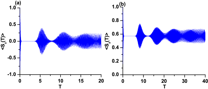
Figure 2: The atomic inversion $\langle S_{z}\left(T\right)\rangle$ against the scaled time $T$ for $(j,\theta)=(150,\pi/3)$ with $\bar{\Delta}=0,$ (a) and $300$ (b).

We have considered in Figs. 1 the case in which $j=150,$ $\bar{\Delta}=0$ and $\theta=\pi/2$. Fig. 1(a) displays the behavior of the function against the time within the interval $T\in[0,150]$. From this figure we can observe long series of the particular type of the revival patterns with rapid fluctuations around the origin. Furthermore, the collapse periods increase as the interaction time increases, too. For a large range of the interaction time $T$, $\langle S_{z}\left(T\right)\rangle$ exhibits more fluctuations and interference between the patterns, which causes the superstructure phenomenon (see Fig. 1(b)). From this figure it is obvious that $\langle\hat{S}_{z}(T)\rangle$ is a periodic function with period $\tau\simeq 480$. This behavior is completely different from that of the JCM eber . In the language of entanglement, the systems $\widetilde{s}$ and $\widetilde{j}$ are periodically disentangled. We’ll get back to this point when we discuss the linear entropy. Now we draw the attention to Figs. 2, where $\theta=\pi/3,j=150$ and $\bar{\Delta}=0,300$. From these figures we can observe the standard RCP, which is quite similar to that of the JCM. The origin in this is the shape of the photon-number distribution of the CSS, which, in this case, is quite similar to that of the coherent state. Moreover, the comparison between Fig. 1(b) and Fig. 2(a) shows that the smoothness of the photon distribution does not always cause the standard RCP. Precisely, this phenomenon, for the system under consideration, depends on the location of the center of symmetrization of the photon-number distribution in the photon-number domain. As a result of this the behavior of the system for $\theta=\pi/2$ is quite different from that of the JCM fle . We proceed, from Fig. 2(a) we can observe long period of collapse after the initial revival pattern. This means that the correlation between the bipartite (, i.e. the $\widetilde{s}$ and $\widetilde{j}$ systems) is weak during this period of the interaction. It is worth reminding that the JCM can generate Schrödinger-cat states in the course of this collapse period cat . Nevertheless, it is difficult to justify this fact for our system. Afterward, the $\langle S_{z}\left(T\right)\rangle$ exhibits a series of the revival patterns, which interfere with each others showing a chaotic behavior. When the effect of the detuning parameter is considered in the interaction, $\bar{\Delta}=300$, the atomic inversion is shifted up and shown fluctuations around $0.6.$ Also we can observe an increase in the revival-pattern series compared to that of the exact resonance case. The shift occurred in the evolution of the $\langle\hat{S}_{z}(T)\rangle$ for the off-resonance case indicates weak entanglement in the bipartite. This point will be elaborated when we discuss the behavior of the linear entropy.

IV Variance squeezing

One of the most important phenomena in the quantum optics is the squeezing, which has been attracted much attention in the last three decades. Thereby, it is reasonable to discuss this phenomenon for the $XX$ central spin model. Precisely, we investigate squeezing for both of the $\widetilde{s}$ and $\widetilde{j}$ systems. In doing so, we assume that $\hat{A}$ and $\hat{B}$ are any two physical observable, which satisfy the commutation relation $\left[\hat{A},\hat{B}\right]=i\hat{C}$. Thus, we have the following uncertainty relation:

$$\langle\left(\Delta\hat{A}\right)^{2}\rangle\langle\left(\Delta\hat{B}\right)^{2}\rangle\geq\frac{1}{4}|\langle\hat{C}\rangle|^{2},$$ (37)

where $\langle\left(\Delta\hat{A}\right)^{2}\rangle=\langle\hat{A}^{2}\rangle-\langle\hat{A}\rangle^{2}$. Therefore, squeezing can be generated in the component $\hat{A}$, say, if the following inequality is satisfied:

$$A=\langle\left(\Delta\hat{A}\right)^{2}\rangle-\frac{|\langle\hat{C}\rangle|}{2}<0.$$ (38)

Similar inequality can be quoted to the operator $\hat{B}$. As well-known, the atomic squeezing is state dependent. If we use different form of the commutation rules, we will get different behavior in the evolution of the squeezing factors. Based on this fact it would be more convenient to investigate these various cases. Precisely, we study squeezing for the cases $(x,y),(x,z)$ and $(y,z)$. For instance, for the $(x,y)$ case of the $\widetilde{s}$ system we mean $\hat{A}=\hat{S}_{x},\hat{B}=\hat{S}_{y}$ and $\hat{C}=\hat{S}_{z}$. The other cases can be similarly expressed. Information about these cases have been shown in Figs. 3–5. We start the discussion with Figs. 3, which have been given to the case $(x,y)$. Generally, we have noted that for the resonance case squeezing can occur only in the $y$-component. This is remarkable from the expressions (28), where $\langle\hat{S}_{x}(T)\rangle=0$ and hence $S_{x}>0$. This indicates that the value of the detuning parameter $\bar{\Delta}$ plays a significant role in the behavior of the atomic squeezing. From Fig. 3(a), i.e. resonance case, one can observe that squeezing occurs only in $S_{y}$ and shows maximum after onset the interaction. As the interaction time increases the amount of squeezing smoothly decreases. Also, the function shows irregular fluctuations. Quite different behavior is observed for the off-resonance case as shown in Fig. 3(b). In this case, the quantity $S_{y}$ exhibits amount of squeezing less than that of the resonance case. Surprisingly, it also exhibits RCP. This is related to the fact that the Rabi oscillation is quite sensitive to the value of $\bar{\Delta}$ (cf. (36)). This phenomenon has been reported earlier in the evolution of the squeezing factors of the Kerr coupler fai .

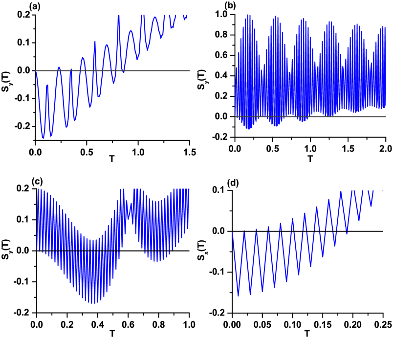
Figure 3: The variances squeezing as indicated for the case $(x,y)$ against the scaled time $T$ when $(j,\theta)=(150,\pi/2)$ with $\bar{\Delta}=0$ (a), $300$ (b), and $100$ (c)-(d). The straight line represents the squeezing bound.

Figs. 3(c) and (d) shed some light on the important role of the $\bar{\Delta}$. From these figures we can observe the occurrence of squeezing in the two components $x$ and $y$. In the $y$-component, squeezing occurs over a range of interaction time broader than that in the $x$-component. Nonetheless, the variance squeezing of the $x$-component displays the maximal squeezing after onset the interaction. The comparison among Figs. 3(a)-(d) confirms the potential for controlling the quantum properties of the system via externally adjustable parameters such as duration of interaction time, detuning, etc. Finally, for $\theta=\pi/3$ we have found that squeezing in the case $(x,y)$ is almost negligible.

Now we draw the attention to Figs. 4 (with $\theta=\pi/2$) and 5 (with $\theta=\pi/3$), which have been given to the cases $(x,z)$ and $(y,z)$. Generally, we have found that the amount of squeezing in the $z$-component is almost negligible. Moreover, for these cases the system can generate squeezing for interaction time larger than that of the $(x,y)$ case. In Figs. 4(a) and 4(b) we present the case $(x,z)$. From these figures, we can observe that squeezing occurs in the $x$-component only after onset the interaction. As the interaction time increases the amount of the squeezing gradually decreases. For the off-resonance case, we can observe the occurrence of the RCP in the evolution of the squeezing function (see Fig. 4(b)). Fig. 4(c) is given for the case $(y,z)$ with strong detuning. From this figure we can observe the occurrence of the long-lived squeezing. Moreover, more fluctuations can be seen in addition to interference between the patterns showing the superstructure phenomenon. Now, we draw the attention to the case $\theta=\pi/3$, which is shown in Figs. 5. For the case $(x,z)$ squeezing occurs only in the resonance case, while for the case $(y,z)$ it occurs in the off-resonance case, i.e. $\bar{\Delta}=300.$ In Fig. 5(a), squeezing is immediately generated after switching on the interaction showing its maximal value. As the interaction proceeds squeezing appears in an oscillatory form, which decreases with increasing the interaction time. This behavior is quite similar to that of the single-atom entropy squeezing of the two two-level atoms interacting with a single-mode quantized electromagnetic field in a lossless resonant cavity fais . The comparison between Fig. 5(a) and Fig. 5(b) shows that squeezing observed for the case $(x,z)$ is stronger than that for the case $(y,z)$. From Figs. (3)-(5) one can conclude that squeezing can be engineered (, i.e. it can be obtained from a specific component) via controlling the interaction parameters.

Figure 4: The variances squeezing as indicated against the scaled time $T$ for $(j,\theta)=(150,\pi/2)$ with $\bar{\Delta}=0$ (a), $300$ (b)–(c). Figures (a) and (b) are given to the case $(x,z)$, while (c) for the case $(y,z)$. The straight line represents the squeezing bound.

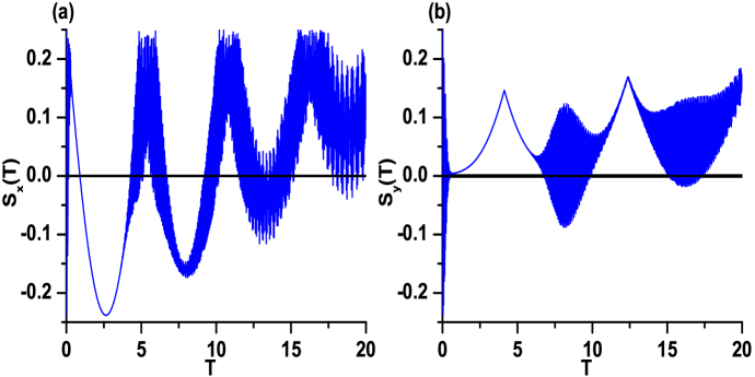
Figure 5: The variances squeezing as indicated against the scaled time $T$ for $(j,\theta)=(150,\pi/3)$ with $\bar{\Delta}=0$ (a) and $300$ (b). Figure (a) is given to the case $(x,z)$, while (b) for the case $(y,z)$. The straight line represents the squeezing bound.

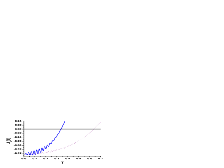
Figure 6: The variance squeezing $J_{x}$ of the angular momentum against the scaled time $T$ where $\left(j,\bar{\Delta},\theta\right)=\left(150,0,\pi/3\right)$ solid curve and $\left(j,\bar{\Delta},\theta\right)=\left(150,300,\pi/3\right)$ dashed curve. The straight line represents the squeezing bound.

Now we turn our attention to discuss the squeezing related to the $\widetilde{j}$ system. For the case $(x,y)$ we have $\hat{A}=\hat{J}_{x},\hat{B}=\hat{J}_{y}$ and $\hat{C}=\hat{J}_{z}$ and the information is shown in Fig. 6. Generally, we have found that squeezing occurs only in the $x$-component. Precisely, the CSS exhibits squeezing for certain values of $\theta$. This initial squeezing gradually decreases and vanishes as the interaction proceeds. Squeezing in the off-resonance case can survive for period of interaction time longer than that of the resonance one. This is obvious when we compare the solid curve to the dashed curve in Fig. 6. The occurrence of the nonclassical effects in the $\widetilde{j}$ system basically depends on the initial state of the $\widetilde{j}$ system physica1 ; physica2 ; physica3 ; physica4 ; physr4 .

V Entanglement

In this section, we investigate the entanglement in the system. Precisely, we demonstrate two type of entanglement; namely central-atom-surroundings entanglement and entanglement among the surrounded spins. Before going into the details there is an important remark we would like to address here. In somehow the interaction mechanism in the system (2) is quite similar to that of the JCM 1 . This is quite obvious if we interchange the bosonic operators by the angular momentum ones, i.e. $(\hat{J}_{-},\hat{J}_{+},\hat{J}_{z})\longrightarrow(\hat{a},\hat{a}^{\dagger},\hat{a}^{\dagger}\hat{a})$. We exploit this fact to use the linear entropy for quantifying the entanglement between the $\widetilde{s}$ and $\widetilde{j}$ systems c ; f . It is worth mentioning that such type of entanglement is completely different from that discussed in physica1 , where the authors have studied the entanglement between two central atoms after tracing over the variables of the surroundings. Now, we start the discussion with the $\widetilde{s}-\widetilde{j}$ entanglement. For this purpose we write down the definition of the linear entropy as c ; f :

$$\eta\left(T\right)=\frac{1}{2}\left[1-\xi^{2}\left(T\right)\right],$$ (39)

where $\xi\left(T\right)$ is the well known a Bloch sphere radius, which has the form:

$$\xi^{2}\left(T\right)=\langle\hat{S}_{x}\left(T\right)\rangle^{2}+\langle\hat{S}_{y}\left(T\right)\rangle^{2}+\langle\hat{S}_{z}(T)\rangle^{2}.$$ (40)

The Bloch sphere is a tool in quantum optics, where the simple qubit state is successfully represented, up to an overall phase, by a point on the sphere, whose coordinates are the expectation values of the atomic set operators of the system. This means that entanglement is strictly related to the behavior of observable of clear physical meaning. The function $\eta(T)$ ranges between $0$ for disentangled bipartite and $1/2$ for maximally entangled ones. In Figs. (7) we have plotted the function $\eta(T)$ against the scaled time $T$ for given values of the interaction parameters. From Fig. 7(a), i.e. $\theta=\pi/2$, as the interaction time increases the decoupled bipartite at $T=0$ becomes entangled. The entanglement gets stronger as the interaction proceeds. Also the function shows rapid fluctuations during the whole duration of the interaction. The bipartite is periodically disentangled with period $\tau\simeq 480$. This in a good agreement with the behavior of the atomic inversion, (see Fig. 1(a)). Now we extend our discussion to the case $\theta=\pi/3$ (see Figs. 7(b)-(c)). For the resonance case, the bipartite exhibits maximal entanglement after switching on the interaction. Afterward, the function $\eta\left(T\right)$ rebounds and decreases its value below $0.4$ around $T\simeq 2.5$ showing partial entanglement, see Fig. 7(b). As the interaction is going on the bipartite exhibits long-lived entanglement. In some sense the behavior of Fig. 7(b) is quite similar to that of the JCM f . Information about the off-resonance case is shown in Fig. 7(c). From this figure we can observe a considerable reduction in the entanglement compared to the previous case. Also this figure exhibits RCP as that of the corresponding atomic inversion. The comparison among Figs. 7(a)–(c) shows that the values of the parameters $\theta$ and $\bar{\Delta}$ play the significant role in the occurrence of the RCP.

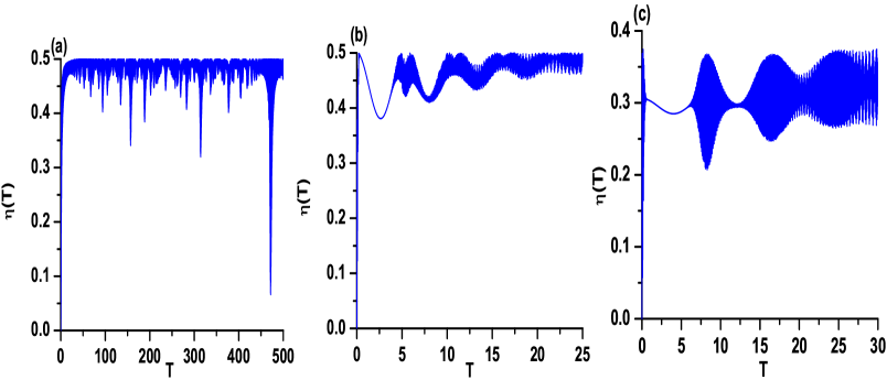
Figure 7: Linear entropy $\eta\left(T\right)$ against the scaled time $T$ for $(j,\bar{\Delta},\theta)=(150,0,\pi/2)$ (a), $(150,0,\pi/3)$ (b), and $(150,300,\pi/3)$ (c).

Now, we close this section by investigating the entanglement among the spins in the $\widetilde{j}$ system. The entanglement among atoms in the $N$-particle system can be amounted by spin squeezing concept as choi ; fs :

$$\bar{\zeta}(T)=\frac{N\langle\left(\Delta\hat{J}_{x}(T)\right)^{2}\rangle}{\langle\hat{J}_{y}(T)\rangle^{2}+\langle\hat{J}_{z}(T)\rangle^{2}},$$ (41)

where $N=2J$. The system shows disentanglement (maximal entanglement) when $\bar{\zeta}\left(T\right)=1\quad(0)$. For the sake of convenience we reformulate the above equation (41) as:

$$\zeta(T)=\langle\left(\Delta\hat{J}_{x}(T)\right)^{2}\rangle-\frac{1}{N}\left[\langle\hat{J}_{y}(T)\rangle^{2}+\langle\hat{J}_{z}(T)\rangle^{2}\right].$$ (42)

Figure 8: Entanglement parameter $\zeta\left(T\right)$ of the angular momentum system in the $x$-direction aganist the scaled time $T$  for $\left(j,\bar{\Delta},\theta\right)=\left(150,0,\pi/3\right)$ solid curve and $\left(150,300,\pi/3\right)$ dash curve.

In this case the limitations become $\zeta(T)=-1$ for maximal entanglement and $0$ for disentanglement. Now we use the formula (42) to examine the behavior of our system. The calculation of different quantities in (42) is already given in section 2. In Fig. 8 we plot $\zeta(T)$ for $(j,\bar{\Delta},\theta)=(150,0,\pi/3)$ (solid curve) and $(150,300,\pi/3)$ (dashed curve). From this figure we can observe that the entanglement instantaneously occurs among the spins only for a short duration of interaction time. The amounts of entanglement in the resonance case are stronger than those in the off-resonance one. Nevertheless, the increase in $\bar{\Delta}$ results in the increase in oscillation frequency of the $\zeta(T)$. This indicates a potential for the quantum control of entanglement properties of the system via externally adjustable parameters. The comparison between the Fig. 6 and the Fig. 8 confirms the fact that the observed squeezing is not always accompanied by an increase in the quantum entanglement among the spins choi . Precisely, quantum squeezing does not necessarily imply entanglement.

VI Conclusion

In this paper, we have studied the quantum properties of the $XX$ central spin model. We have mange to solve the Heisenberg equations of motion for the Pauli spin operators and the angular momentum ones. We have considered that the $\widetilde{s}$ and $\widetilde{j}$ systems are initially prepared in the excited state and the CSS, respectively. We have investigated the atomic inversion, the variance squeezing and the entanglement. The results can be summarized as follows. The atomic inversion can exhibit RCP for certain values of the interaction parameters. Precisely, the occurrence of the RCP is sensitive not only to the smoothness of the photon distribution but also to its location of the symmetrization center in the photon-number domain. Squeezing is available only in the $x$ and $y$ components of the Puali spin operators. Also controlling the value of $\bar{\Delta}$ can lead to the occurrence of the RCP in the atomic squeezing. Squeezing can occur in the $\widetilde{j}$ system only when CSS is initially squeezed. The entanglement between the bipartite $\widetilde{s}$ and $\widetilde{j}$ is sensitive to the value of $\theta$. For instance, when $\theta=\pi/2$ the bipartite becomes periodically disentangled. Increasing the value of $\bar{\Delta}$ leads to decreasing the entanglement in the bipartite. Entanglement among the spins of the $\widetilde{j}$ system occurs for short duration of the interaction time. Also quantum squeezing does not necessarily imply entanglement.

Acknowledgement:

One of us (M.S.A.) is grateful for the financial support from the project Math 2010/32 of the Research Centre, College of Science, King Saud University.

References

- (1) A. Bayat, S. Bose, Phys. Rev. A, 75 (2007) 022321; V. Kostak, G.M. Nikolopoulos, I. Jex, Phys. Rev. A, 75 (2007) 042319; M.B. Plenio, S. Virmani, Phys. Rev. Lett., 99 (2007) 120504.
- (2) E.H. Lieb, T.D. Schultz, D.C. Mattis, Ann. Phys. (N.Y.), 16 (1961) 407; L. Amico, A. Osterloh, F. Plastina, G. Palma, R. Fazio, Phys. Rev. A, 69 (2004) 022304; V. Subrahmayam, Phys. Rev. A, 69 (2004) 034304; L. C. Venuti, M. Roncaglia, Phys. Rev. A, 81 (2010) 060101(R).
- (3) B.-Q. Jin, V.E. Korepin, J. Stat. Phys., 116 (2004) 79; A.R. Its, B.-Q. Jin, V.E. Korepin, J. Phys. A: Math. Gen., 38 (2005) 2975; A. Sen, U. Sen, M. Lewenstein, Phys. Rev. A, 70 (2004) 060304; J. Fitzsimons, J. Twamley, Phys. Rev. A, 72 (2005) 050301(R).
- (4) G. De Chiara, S.Montangero, P. Calabrese, R. Fazio, J. Stat.Mech.:Theo. and Exper., (2005) P 03001.
- (5) J.S. Pratt, Phys. Rev. A, 69 (2004) 042312; G.L. Kamta, A. Starace, Phys. Rev. Lett., 88 (2002) 10; S. Hamieh, M.I. Katsnelson, Phys. Rev. A, 72 (2005) 032316; P. Karbach, J. Stolze, Phys. Rev. A, 72 (2005) 030301; D. Bruß, N. Datta, A. Ekert, L.C. Kwek, C. Machiavello, Phys. Rev. A, 72 (2005) 014301; A. Hutton, S. Bose, Phys. Rev. Lett., 93 (2004) 237205; X.-Z. Yuan, H.-S. Goan, K.-D. Zhu, Phys. Rev. B, 75 (2007) 045331; Y. Hamdouni, M. Fannes, F. Petruccione, Phys. Rev. B, 73 (2006) 245323.
- (6) F. Verstraete, M. Popp, J.I. Cirac, Phys. Rev. Lett., 92 (2004) 027901; M.C. Arnesen, S. Bose, V. Vedral, Phys. Rev. Lett., 87 (2001) 017901; J.S. Pratt, Phys. Rev. Lett., 93 (2004) 237205; E. Ferraro, A. Napoli, M.A. Jivulescu, A. Messina, Eur. Phys. J. Special Topics, 160 (2008) 157.
- (7) S. Bose, Phys. Rev. Lett., 91 (2003) 207901.
- (8) G. De. Chiara, R. Fazio, C. Macchiavello, S. Montangero, G. M. Palma, Phys. Rev. A, 72 (2005) 012328.
- (9) A. Imamoglu et al, Phys. Rev. Lett., 83 (1999) 4204.
- (10) V. Privman, I. D. Vagner, G. Kventsel, Phys. Lett. A, 239 (1998) 141.
- (11) A. Hutton, S. Bose, Phys. Rev. A, 69 (2004) 042312.
- (12) A. Sorensen, K. Molmer, Phys. Rev. Lett., 83 (1999) 2274.
- (13) M. Gaudin, Le journal de Physique, 10 (1976) 1087.
- (14) M. A. Jivulescu, E. Ferraro, A. Napoli, A. Messina, Phys. Scr., (2009) T135.
- (15) E. Ferraro, A. Napoli, M. Guccione, A. Messina, Phys. Scr., (2009) 014032.
- (16) E. Ferraro, H.-P. Breuer, A. Napoli, M. A. Jivulescu, A. Messina, Phys. Rev. B, 78 (2008) 064309.
- (17) M.A. Jivulescu, E. Ferraro, A. Napoli, A. Messina, Rep. on Math. Phys., 64 (2009) 315.
- (18) H.-P. Breuer, D. Burgarth, F. Petruccione, Phys. Rev. B, 70 (2004) 045323; Y. Hamdouni, M. Fannes, F. Petruccione, Phys. Rev. B, 73 (2006) 245323; Y. Hamdouni, F. Petruccione, Phys. Rev. B, 76 (2007) 174306.
- (19) F. T. Arrechi, E. Courtens, R. Gilmore, H. Thomas, Phys. Rev. A, 6 (1972) 2211; S. M. Barnett, P. M. Radmore, Methodes in Theoretical Quantum Optics(Oxford University Press, Oxford, 1997); R. N. Deb, M.S. Abdalla, S. S. Hassan, N. Nayak, Phys. Rev.A, 73 (2006) 053817.
- (20) S. Choi, N. P. Bigelow, Phys. Rev. A, 72 (2005) 033612.
- (21) E. T. Jayness, F.W. Cummings, Proc. IEEE, 51 (1963) 89.
- (22) J. H. Eberly, N. B. Narozhny, J. J. Sanchez-Mondragon, Phys. Rev. Lett., 44 (1980) 1323; N. B. Narozhny, J. J. Sanchez-Mondragon, J. H. Eberly, Phys. Rev. A, 23 ( 1981) 236; H. I. Yoo, J. J. Sanchez-Mondragon, J. H. Eberly, J. Phys. A: Math. Gen., 14 (1981) 1383 ; H. I. Yoo, J. H. Eberly, Phys. Rep., 118 (1981) 239.
- (23) M. Fleischhauer, W. P. Schleich, Phys. Rev. A, 47 (1993) 4258.
- (24) F. A. A. El-Orany, A.-S. Obada, J. Opt. B: Quantum Semiclass. Opt. 4 (2002) 121.
- (25) F. A. A. El-Orany, M. Sebawe Abdalla, J. Peřina, J. Opt. B: Quantum Semiclass. Opt., 6 (2004) 460; F. A. A. El-Orany, M. S. Abdalla , J. Peřina, Eur. Phys. J. D, 33 (2005) 453.
- (26) F. A. A. El-Orany, M. R. B. Wahiddin, A.-S. F. Obada, Opt. Commun., 281 (2008) 2854.
- (27) C.C.Gerry, P.L. Knight, Introductory Quantum Optics; Cambridge University Press: Cambridge, 2005; pp 108110; Appendix A.
- (28) F. A. A. El-Orany, J. Mod.Opt., 56 (2009) 117.
- (29) A. Sorensen, L.-M. Duan, J. I. Cirac, P. Zoller, Nature (London), 409 (2001) 63; A. Micheli, D. Jaksch, J. I. Cirac, P. Zoller, Phys. Rev. A, 67 (2003) 013607.