Four-nucleon scattering with a correlated Gaussian basis method

Abstract

Elastic-scattering phase shifts for four-nucleon systems are studied in an $ab$-$initio$ type cluster model in order to clarify the role of the tensor force and to investigate cluster distortions in low energy $d$+$d$ and $t$+$p$ scattering. In the present method, the description of the cluster wave function is extended from a simple (0$s$) harmonic-oscillator shell model to a few-body model with a realistic interaction, in which the wave function of the subsystems are determined with the Stochastic Variational Method. In order to calculate the matrix elements of the four-body system, we have developed a Triple Global Vector Representation method for the correlated Gaussian basis functions. To compare effects of the cluster distortion with realistic and effective interactions, we employ the AV8^′ potential as a realistic interaction and the Minnesota potential as an effective interaction. Especially for ${}^{1}S_{0}$, the calculated phase shifts show that the $t$+$p$ and $h$+$n$ channels are strongly coupled to the $d$+$d$ channel for the case of the realistic interaction. On the contrary, the coupling of these channels plays a relatively minor role for the case of the effective interaction. This difference between both potentials originates from the tensor term in the realistic interaction. Furthermore, the tensor interaction makes the energy splitting of the negative parity states of ⁴He consistent with experiments. No such splitting is however reproduced with the effective interaction.

1 Introduction

The microscopic cluster model is one of the successful models to study the structure and reactions of light nuclei [1]. In the conventional cluster model, one assumes that the nucleus is composed of several simple clusters with $A\leq 4$ which are described by (0$s$) harmonic-oscillator shell model functions, and use an effective $N$-$N$ interaction which is appropriate for such a model space. However, it is well known that the ground states of the typical clusters $d$, $t$, $h$ and ⁴He have non-negligible admixtures of $D$-wave component due to the tensor interaction. Since the conventional cluster model does not directly treat the $D$-wave component, the strong attraction of the nucleon-nucleon interaction due to the tensor term is assumed to be renormalized into the central term of the effective interaction.

Recently, $ab$-$initio$ structure calculations [2] have been successfully developed: Stochastic Variational Method (SVM) [3, 4, 5, 6], Global Vector Representation method (GVR) [7, 8], Green’s function Monte Carlo method [9], no core shell model [10], correlated hyperspherical harmonics method [11], unitary correlation operator method [12], and so on. Although the application of $ab$-$initio$ reaction calculations with a realistic interaction are restricted so much in comparison with structure calculations, it has been intensively applied to the four-nucleon systems $t$+$n$ and $h$+$p$ [13, 14, 15, 16, 17, 18, 19]. Especially $d$+$d$ scattering states, which couple to $t$+$p$ and $h$+$n$ channels, have attracted much attention, because the $d$+$d$ radiative capture is one of the mechanisms making ⁴He through electro-magnetic transitions [20, 21] and also have posed intriguing puzzles for analyzing powers [22, 23, 24, 25, 26], which are motivated by the famous $A_{y}$ problem in the three-nucleon system.

Furthermore, the $d$+$d$ elastic-scattering phase shifts are interesting because the astrophysical S-factor of the $d$($d$,$\gamma$)⁴He reaction is not explained by any calculation using an effective interaction that contains no tensor term, and is expected to be contributed by the $D$-wave components of the clusters through $E2$ transitions [27, 28].

Also, thanks to recent developments of the microscopic cluster model, the simple model using the (0$s$) harmonic-oscillator wave function with an effective interaction is not mandatory any more, at least, in light nuclei. We can use a kind of $ab$-$initio$ cluster model which employs more realistic cluster wave functions with realistic interactions. Therefore, it is interesting to see the difference between the $ab$-$initio$ reaction calculations with a tensor term and the conventional cluster model calculations without a tensor term in few-body systems.

The microscopic $R$-matrix method (MRM) with a cluster model (GCM or RGM) has been applied to studies of many nuclei [29, 30, 31, 32]. It is now used in $ab$ $initio$ descriptions of collisions [16]. We have also applied the MRM to the $h$+$p$ scattering problem with more realistic cluster wave functions by using a realistic interaction [13]. The Gaussian basis functions for the expansion of the cluster wave functions are chosen by a technique of the SVM [5]. In the MRM, as will be shown later, the relative wave function between clusters ($a$ and $b$) is connected to the boundary condition at a channel radius. The problem is how to calculate the matrix elements. In this paper, we develop a method called the Triple Global Vector Representation method (TGVR), by which we calculate the matrix elements in a unified way. Although we restricted ourselves to four nucleon systems in the present paper, the formulation of the TGVR itself can be applied to more than four-body systems as in the previous studies of the Global Vector Representation methods (GVR) [8]. Furthermore, for scattering problems, the TGVR can deal with more complicated systems than the double (or single) global vector which was given in the previous papers [7, 8], because we need three representative orbital angular momenta, the total internal orbital momenta of both clusters and the orbital momentum of their relative motion, in order to reasonably describe the scattering states. In other words, the first global vector represents the angular momentum of cluster $a$, the second global vector represents the angular momentum of cluster $b$, and the third global vector represents the relative angular momentum between the clusters.

In this paper, we will investigate the effect of the distortion of clusters on the $d$+$d$ elastic-scattering by comparing the phase shifts calculated with a realistic and an effective interaction. In section 2, we explain the MRM in brief. In section 3, the correlated Gaussian (CG) method with the TGVR, which has newly been developed for the present analysis, will be presented. In section 4, we will explain how to calculate the matrix elements with TGVR basis functions. The typical matrix elements are also given in the appendix. In section 5, we will present and discuss the calculated scattering phase shifts in detail. Finally, summary and conclusions are given in section 6.

2 Microscopic $R$-matrix method

In the present study we calculate $d$+$d$ and $t$+$p$ (and $h$+$n$) elastic scattering phase shifts with the microscopic $R$-matrix method. Though the method is well documented in e.g. Refs. [29, 30, 32], we briefly explain it below in order to present definitions and equations needed in the subsequent sections. Since our interest is on low-energy scattering, we consider only two-body channels. A channel $\alpha$ is specified by the two nuclei (clusters) $a,b$, their angular momenta, $I_{a},I_{b}$, the channel spin $I$ that is a resultant of the coupling of $I_{a}$ and $I_{b}$, and the orbital angular momentum $\ell$ for the relative motion of $a$ and $b$. The wave function of channel $\alpha$ with the total angular momentum $J$, its projection $M$, and the parity $\pi$ takes the form

$$\Psi^{JM\pi}_{\alpha}={\cal A}\left[\left[\Phi^{a}_{I_{a}}\Phi^{b}_{I_{b}}\right]_{I}\chi_{\alpha}(\mbox{\boldmath$\rho$}_{\alpha})\right]_{JM},$$ (1)

where $\Phi^{a}_{I_{a}}$ and $\Phi^{b}_{I_{b}}$ are respectively antisymmetrized intrinsic wave functions of $a$ and $b$, and ${\cal A}$ is an operator that antisymmetrizes between the clusters. The square bracket $[{I_{a}}\ {I_{b}}]_{I}$ denotes the angular momentum coupling. The coordinate ${\mbox{\boldmath$\rho$}}_{\alpha}$ in the relative motion function $\chi^{J}_{\alpha}$ is the relative distance vector of the clusters. The channel spin $I$ and the relative angular momentum $\ell$ in $\alpha$ are coupled to give the total angular momentum $J$. The relative-motion functions $\chi_{\alpha}$ also depend on $J$ and $\pi$. For simplicity, this dependence is not displayed explicitly in the notation for $\chi_{\alpha}$ as well as for some other quantities below.

The configuration space is divided into two regions, internal and external, by the channel radius $a$. In the internal region ($\rho_{\alpha}\leq a$), the total wave function may be expressed in terms of a combination of various $\Psi_{\alpha}^{JM\pi}$s

$$\Psi^{JM\pi}_{\rm int} = \sum_{\alpha}\Psi^{JM\pi}_{\alpha}$$ (2)

$$= \sum_{\alpha}\sum_{n}f_{\alpha n}{\cal A}u_{\alpha n}(\rho_{\alpha})\phi^{JM\pi}_{\alpha},$$

with

$$\phi^{JM\pi}_{\alpha}=\frac{1}{\sqrt{(1+\delta_{I_{a}I_{b}}\delta_{ab})(1+\delta_{ab})}}\left\{\left[\left[\Phi^{a}_{I_{a}}\Phi^{b}_{I_{b}}\right]_{I}Y_{\ell}(\widehat{\mbox{\boldmath$\rho$}}_{\alpha})\right]_{JM}\right.$$

$$\left.+(-1)^{A_{a}+I_{a}+I_{b}-I+\ell}\left[\left[\Phi^{b}_{I_{b}}\Phi^{a}_{I_{a}}\right]_{I}Y_{\ell}(\widehat{\mbox{\boldmath$\rho$}}_{\alpha})\right]_{JM}\delta_{ab}\right\},$$ (3)

where $A_{a}$ is the number of nucleons in cluster $a$, $\delta_{ab}$ is unity if $a$ and $b$ are identical clusters and zero otherwise, and $\delta_{I_{a}I_{b}}$ is unity if the clusters are in identical states and zero otherwise. In the second line of Eq. (2), the relative motion functions of Eq. (1) are expanded in terms of some basis functions as

$$\chi_{\alpha m}({\mbox{\boldmath$\rho$}}_{\alpha})=\sum_{n}f_{\alpha n}u_{\alpha n}(\rho_{\alpha})Y_{\ell m}(\widehat{\mbox{\boldmath$\rho$}}_{\alpha}).$$ (4)

In what follows we take

$$u_{\alpha n}(\rho_{\alpha})=\rho_{\alpha}^{\ell}\exp(-\frac{1}{2}\lambda_{n}\rho_{\alpha}^{2})$$ (5)

with a suitable set of $\lambda_{n}$s.

In the external region ($\rho_{\alpha}\geq a$), the total wave function takes the form

$$\Psi^{JM\pi}_{\rm ext}=\sum_{\alpha}g_{\alpha}(\rho_{\alpha})\phi^{JM\pi}_{\alpha}.$$ (6)

Note that the antisymmetrization between the clusters is dropped in the external region under the condition that the channel radius $a$ is large enough. The function $g_{\alpha}(\rho_{\alpha})$ of Eq. (6) is a solution of the equation

$$\left[-\frac{\hbar^{2}}{2\mu_{\alpha}}\left(\frac{d^{2}}{d\rho_{\alpha}^{2}}+\frac{2}{\rho_{\alpha}}\,\frac{d}{d\rho_{\alpha}}-\frac{\ell(\ell+1)}{\rho_{\alpha}^{2}}\right)+\frac{Z_{a}Z_{b}e^{2}}{\rho_{\alpha}}\right]g_{\alpha}(\rho_{\alpha})=E_{\alpha}g_{\alpha}(\rho_{\alpha}),$$ (7)

where $\mu_{\alpha}$ is the reduced mass for the relative motion in channel $\alpha$, $Z_{a}e$ and $Z_{b}e$ are the charges of $a$ and $b$, and $E_{\alpha}=E-E_{a}-E_{b}$ is the energy for the relative motion, where $E$ is the total energy, and $E_{a}$ and $E_{b}$ are the internal energies for the clusters $a$ and $b$, respectively. For the scattering initiated through the channel $\alpha_{0}$, the asymptotic form of $g_{\alpha}$ for the open channel $\alpha$ $(E_{\alpha}\geq 0)$ is

$$g_{\alpha}(\rho_{\alpha})=v_{\alpha}^{-1/2}\rho_{\alpha}^{-1}[I_{\alpha}(k_{\alpha}\rho_{\alpha})\delta_{\alpha\,\alpha_{0}}-S_{\alpha\,\alpha_{0}}^{J\pi}O_{\alpha}(k_{\alpha}\rho_{\alpha})],$$ (8)

where $k_{\alpha}=\sqrt{2\mu_{\alpha}|E_{\alpha}|}/\hbar$, $v_{\alpha}=\hbar k_{\alpha}/\mu_{\alpha}$ and $S_{\alpha\,\alpha_{0}}^{J\pi}$ is an element of the $S$-matrix (or collision matrix) to be determined. Here $I_{\alpha}(k_{\alpha}\rho_{\alpha})$ and $O_{\alpha}(k_{\alpha}\rho_{\alpha})$ are the incoming and outgoing waves defined by

$$I_{\alpha}(k_{\alpha}\rho_{\alpha})=O_{\alpha}(k_{\alpha}\rho_{\alpha})^{*}=G_{\ell}(\eta_{\alpha},k_{\alpha}\rho_{\alpha})-iF_{\ell}(\eta_{\alpha},k_{\alpha}\rho_{\alpha}),$$ (9)

with the regular and irregular Coulomb functions $F_{\ell}$ and $G_{\ell}$. The Sommerfeld parameter $\eta_{\alpha}$ is $\mu_{\alpha}Z_{a}Z_{b}e^{2}/\hbar^{2}k_{\alpha}$. For a closed channel $\alpha$ $(E_{\alpha}<0)$, the asymptotic form of $g_{\alpha}$ is given by the Whittaker function

$$g_{\alpha}(\rho_{\alpha})\propto\rho_{\alpha}^{-1}W_{-\eta_{\alpha},\ell+1/2}(2k_{\alpha}\rho_{\alpha}).$$ (10)

The matrix elements $S_{\alpha\alpha_{0}}^{J\pi}$ are determined by solving a Schrödinger equation with a microscopic Hamiltonian $H$ involving the $A_{a}+A_{b}$ nucleons,

$$(H+{\cal L}-E)\Psi_{\rm int}^{JM\pi}={\cal L}\Psi_{\rm ext}^{JM\pi},$$ (11)

with the Bloch operator ${\cal L}$

$${\cal L}=\sum_{\alpha}\frac{\hbar^{2}}{2\mu_{\alpha}a}|\phi_{\alpha}^{JM\pi}\rangle\delta(\rho_{\alpha}-a)\left(\frac{\partial}{\partial\rho_{\alpha}}-\frac{b_{\alpha}}{\rho_{\alpha}}\right)\rho_{\alpha}\langle\phi_{\alpha}^{JM\pi}|,$$ (12)

where the channel radius $a$ is chosen to be the same for all channels, and the $b_{\alpha}$ are arbitrary constants. Here, we choose $b_{\alpha}=0$ for the open channels and $b_{\alpha}=2k_{\alpha}aW^{\prime}_{-\eta_{\alpha},\ell+1/2}(2k_{\alpha}a)/W_{-\eta_{\alpha},\ell+1/2}(2k_{\alpha}a)$ for the closed channels. The results do not depend on the choices for $b_{\alpha}$ but these values simplify the calculations. Notice that the projector on $|\phi_{\alpha}^{JM\pi}\rangle$ in Eq. (12) is not essential in a microscopic calculation and can be dropped since the various channels are orthogonal at the channel radius.

The Bloch operator ensures that the logarithmic derivative of the wave function is continuous at the channel radius. In addition, $\Psi_{\rm int}^{JM\pi}$ must be equal to $\Psi_{\rm ext}^{JM\pi}$ at $\rho_{\alpha}=a$. Projecting the Schrödinger equation on a basis state, one obtains

$$\sum_{\alpha n}C_{\alpha^{\prime}n^{\prime},\alpha n}\,f_{\alpha n}=\langle\Phi_{\alpha^{\prime}n^{\prime}}^{JM\pi}|{\cal L}|\Psi_{\rm ext}^{JM\pi}\rangle$$ (13)

with

$$C_{\alpha^{\prime}n^{\prime},\alpha n}=\langle\Phi_{\alpha^{\prime}n^{\prime}}^{JM\pi}|H+{\cal L}-E|{\cal A}\Phi_{\alpha n}^{JM\pi}\rangle_{\rm int},$$ (14)

and

$$\Phi_{\alpha n}^{JM\pi}=u_{\alpha n}(\rho_{\alpha})\phi_{\alpha}^{JM\pi}.$$ (15)

Here $\langle|{\cal O}|\rangle_{\rm int}$ indicates that the integration with respect to $\rho_{\alpha}$ is to be carried out in the internal region. Actually $\langle|{\cal O}|\rangle_{\rm int}$ is obtained by calculating the matrix element $\langle|{\cal O}|\rangle$ in the entire space and subtracting the corresponding external matrix element $\langle|{\cal O}|\rangle_{\rm ext}$ that is easily obtained because no intercluster antisymmetrization is needed. The $R$-matrix and $Z$-matrix are defined by

$${\cal R}_{\alpha^{\prime}\alpha}\equiv\frac{\hbar^{2}a}{2}\left(\frac{k_{\alpha^{\prime}}}{\mu_{\alpha^{\prime}}\mu_{\alpha}k_{\alpha}}\right)^{\frac{1}{2}}\sum_{n^{\prime}n}u_{\alpha^{\prime}n^{\prime}}(a)(C^{-1})_{\alpha^{\prime}n^{\prime},\alpha n}u_{\alpha n}(a),$$ (16)

$${\cal Z}_{\alpha^{\prime}\alpha}\equiv I_{\alpha}(k_{\alpha}a)\delta_{\alpha^{\prime}\alpha}-{\cal R}_{\alpha^{\prime}\alpha}k_{\alpha}aI^{\prime}_{\alpha}(k_{\alpha}a).$$ (17)

The $S$-matrix is finally obtained as

$$S^{J\pi}=({\cal Z}^{*})^{-1}{\cal Z}.$$ (18)

In this paper we focus on the elastic phase shifts $\delta_{\alpha}^{J\pi}$ that are defined by the diagonal elements of the $S$-matrix,

$$S_{\alpha\alpha}^{J\pi}=\eta_{\alpha}^{J\pi}e^{2i\delta_{\alpha}^{J\pi}}.$$ (19)

We study four-nucleon scattering involving the $d$+$d$, $t$+$p$ and $h$+$n$ channels in the energy region around and below the $d$+$d$ threshold. In Table 1 we list all possible labels ${}^{2I+1}\ell_{J}$ of physical channels for $J^{\pi}=0^{\pm}$, $1^{\pm}$, and $2^{\pm}$, assuming $\ell\leq 2$. Here “physical” means that the channels involve the cluster bound states that appear in the external region as well. Non-physical channels involving excited pseudo states will also be included in most calculations. Note that the $d$+$d$ channel must satisfy the condition of $I+\ell$ even (see Eq. (3)). The channel spin $I=0$ or 2 can couple with only even $\ell$, but $I=1$ with only odd $\ell$. It is noted that the relative motion for the $d$+$d$ scattering can have $\ell=0$ only when $J^{\pi}$ is equal to $0^{+}$ and $2^{+}$.

Table 1: Channel spins (${}^{2I+1}\ell_{J}$) of physical $d$+$d$, $t$+$p$, and $h$+$n$ channels for $J\leq 2$ and $\ell\leq 2$.

	0+	1+	2+	0-	1-	2-
$d(1^{+})$+$d(1^{+})$	${}^{1}S_{0}$	${}^{5}D_{1}$	${}^{5}S_{2}$	${}^{3}P_{0}$	${}^{3}P_{1}$	${}^{3}P_{2}$
	${}^{5}D_{0}$		${}^{1}D_{2}$
			${}^{5}D_{2}$
$t(\frac{1}{2}^{+})$+$p(\frac{1}{2}^{+}),\;h(\frac{1}{2}^{+})$+$n(\frac{1}{2}^{+})$	${}^{1}S_{0}$	${}^{3}S_{1}$	${}^{1}D_{2}$	${}^{3}P_{0}$	${}^{1}P_{1}$	${}^{3}P_{2}$
		${}^{3}D_{1}$	${}^{3}D_{2}$		${}^{3}P_{1}$

Because one of our purposes in this investigation is to understand the role of the tensor force played in the four-nucleon dynamics, we want to compare the phase shifts obtained with two Hamiltonians that differ in the type of $NN$ interactions. One is a realistic interaction called the AV8^′ potential [33] that includes central, tensor and spin-orbit components. We also add an effective three-nucleon force (TNF) in order to reproduce reasonably the binding energies of $t$, $h$ and ⁴He [34], which makes reasonable thresholds. In the present calculation, the TNF is included in all calculations for AV8^′. Another is an effective central interaction called the Minnesota (MN) potential [35], which reproduce reasonably the binding energies of $t$, $h$ and ⁴He, though it has central terms alone (with an exchange parameter $u=1$). The Coulomb potential is included for both potentials.

The intrinsic wave function $\Phi^{k}_{I_{k}}$ of cluster $k$ $(k=a,\ b)$ is described with a combination of $N_{k}$ basis functions with different $L_{k}$ and $S_{k}$ values

$$\Phi_{I_{k}M_{I_{k}}}^{k}=\sum^{N_{k}}{\cal A}\left[\psi_{L_{k}}^{(\rm{space})}\psi_{S_{k}}^{(\rm{spin})}\right]_{I_{k}M_{I_{k}}}\psi^{(\rm{isospin})}_{T_{k}M_{T_{k}}},$$ (20)

where $\psi_{L_{k}}^{(\rm{space})}$, $\psi_{S_{k}}^{(\rm{spin})}$ and $\psi_{T_{k}M_{T_{k}}}^{(\rm{isospin})}$ denote the space, spin and isospin parts of the cluster wave function. In the case of the AV8^′ potential, the $t$ (or $h$) wave function is approximated with thirty Gaussian basis functions that include $L_{k}\leq 2$, and $S_{k}=\frac{1}{2}$ and $\frac{3}{2}$. The deuteron wave function is also approximated with Gaussian basis functions, four terms both in the $S$- and $D$-waves, respectively. The falloff parameters of the Gaussian functions are selected using the SVM [5] and the expansion coefficients are determined by diagonalizing the intrinsic cluster Hamiltonian. A similar procedure is applied to the case of the MN potential.

The calculated energies $E$, root-mean-square (rms) radii $R^{\rm rms}$ and $D$ state probabilities $P_{D}$ are given in the fourth to sixth columns in Table 2. We use the truncated basis in order to obtain the phase shifts in reasonable computer times, they slightly deviate from more elaborate calculations, which are given in the last three columns. Fortunately, except for the small shift of the threshold energy, the phase shifts are not very sensitive to the details of the cluster wave functions because they are determined by the change of the relative motion function of the clusters. The $N_{k}$ values in parenthesis for ⁴He are the number of $J^{\pi}=0^{+}$ basis functions in the major multi-channel calculation. The energy of ⁴He calculated in Table 2 with the multi-channel calculation is thus not optimized but found to be very close to that of the more extensive calculation. It is noted that the calculated $R^{\rm rms}$ value for the deuteron is smaller than in other calculations. This is due to the restricted choice of the length parameters of the basis functions, which permits us to use a relatively small channel radius of $a\sim 15$ fm. We have checked that the phase shifts for a $d+d$ single channel calculation do not change even when more extended deuteron wave functions are employed.

Table 2: Energies $E$, rms radii $R^{\rm rms}$ and $D$-state probabilities $P_{D}$ of the clusters that appear in four-nucleon scattering and ⁴He with the AV8^′ (with TNF) and MN potentials. $N_{k}$ is the number of basis functions used to approximate the wave function of cluster $k$. The values in the last three columns for three- and four-body systems are taken from Ref. [34] for AV8^′ and Ref. [7] for MN.

potential	cluster	present				literature
		$N_{k}$	$E$	$R^{\rm rms}$	$P_{D}$	$E$	$R^{\rm rms}$	$P_{D}$
			(MeV)	(fm)	($\%$)	(MeV)	(fm)	($\%$)
	$d(1^{+})$	8	$-$2.18	1.79	5.9	$-$2.24	1.96	5.8
AV8′	$t(\frac{1}{2}^{+})$	30	$-$8.22	1.69	8.4	$-$8.41	-	-
(with TNF)	$h(\frac{1}{2}^{+})$	30	$-$7.55	1.71	8.3	$-$7.74	-	-
	4He$(0^{+})$	(2370)	$-$27.99	1.46	13.8	$-$28.44	-	14.1
	$d(1^{+})$	4	$-$2.10	1.63	0	$-$2.20	1.95	0
MN	$t(\frac{1}{2}^{+})$	15	$-$8.38	1.70	0	$-$8.38	1.71	0
	$h(\frac{1}{2}^{+})$	15	$-$7.70	1.72	0	$-$7.71	1.74	0
	4He$(0^{+})$	(1140)	$-$29.94	1.41	0	$-$29.94	1.41	0

3 Correlated Gaussian function with triple global vectors

As explained in the previous section, the calculation of the $S$-matrix reduces to that of the Hamiltonian and overlap matrix elements with the functions defined by (1) and (20), and it is conveniently performed by transforming that wave function into an $LS$-coupled form,

$${\cal A}\left[\left[\left[\psi^{(\rm space)}_{L_{a}}\psi^{(\rm space)}_{L_{b}}\right]_{L_{ab}}\chi_{\alpha}({\mbox{\boldmath$\rho$}}_{\alpha})\right]_{L}\left[\psi^{(\rm spin)}_{S_{a}}\psi^{(\rm spin)}_{S_{b}}\right]_{S}\right]_{JM}.$$ (21)

The transformation can be done as

$${}{\cal A}\left[\left[[\psi_{L_{a}}^{(\rm{space})}\psi_{S_{a}}^{(\rm{spin})}]_{I_{a}}[\psi_{L_{b}}^{(\rm{space})}\psi_{S_{b}}^{(\rm{spin})}]_{I_{b}}\right]_{I}\chi_{\alpha}({\mbox{\boldmath$\rho$}}_{\alpha})\right]_{JM}\psi^{(\rm{isospin})}_{T_{a}M_{T_{a}}}\psi^{(\rm{isospin})}_{T_{b}M_{T_{b}}}$$ (26)

$$= \sum_{L_{ab}LS}\left[\begin{array}[]{ccc}L_{a}&S_{a}&I_{a}\\ L_{b}&S_{b}&I_{b}\\ L_{ab}&S&I\\ \end{array}\right](-1)^{L_{ab}+J-I-L}U(SL_{ab}J\ell;IL)$$

$$\times{\cal A}\left[\psi_{L_{a}L_{b}(L_{ab})\ell L}^{(\rm space)}\left[\psi^{(\rm spin)}_{S_{a}}\psi^{(\rm spin)}_{S_{b}}\right]_{S}\right]_{JM}\psi^{(\rm{isospin})}_{T_{a}M_{T_{a}}}\psi^{(\rm{isospin})}_{T_{b}M_{T_{b}}}$$

with

$$\psi_{L_{a}L_{b}(L_{ab})\ell L}^{(\rm space)}=\left[\left[\psi^{(\rm space)}_{L_{a}}\psi^{(\rm space)}_{L_{b}}\right]_{L_{ab}}\chi_{\alpha}({\mbox{\boldmath$\rho$}}_{\alpha})\right]_{L},$$ (27)

where $U$ and $[\ \ ]$ are Racah and 9$j$ coefficients in unitary form [5].

The evaluation of the matrix element can be done in the spatial, spin, and isospin parts separately. The spin and isospin parts are obtained straightforwardly. In the following we concentrate on the spatial matrix element. The spatial part (27) of the total wave function is given as a product of the cluster intrinsic parts and their relative motion part. The coordinates used to describe the $2N$+$2N$ channel are depicted in Fig. 1(a) with ${\mbox{\boldmath$\rho$}}_{\alpha}={\mbox{\boldmath$x$}}_{3}$, whereas the coordinates suitable for the $t$+$p$ and $h$+$n$ channels are shown in Fig. 1(b) with ${\mbox{\boldmath$\rho$}}_{\alpha}={\mbox{\boldmath$x$}}_{3}^{\prime}$. These coordinate sets are often called H-type and K-type. Therefore the calculation of the spatial matrix element requires a coordinate transformation involving the angular momenta $L_{a},L_{b},\ell$ and $L_{ab}$. Moreover the permutation operator in ${\cal A}$ causes a complicated coordinate transformation. All these complexities are treated elegantly by introducing a correlated Gaussian [36, 6, 5], provided each part of $\psi_{L_{a}L_{b}(L_{ab})\ell L}^{(\rm space)}$ is given in terms of (a combination of) Gaussian functions as in the present case. In what follows we will demonstrate how it is performed. Because the formulation with the correlated Gaussian is not restricted to four nucleons but can be applied to a system including more particles, the number of nucleons is assumed to be $N$ in this and next sections as well as in Appendices B and C unless otherwise mentioned.

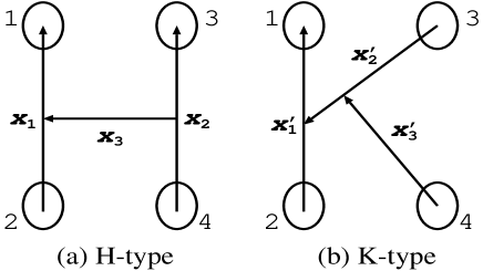
Figure 1: Relative coordinates for the four-body system

The relative and center of mass coordinates of the $N$ nucleons, ${\mbox{\boldmath$x$}}_{i}\,(i=1,\ldots,N)$, and the single-particle coordinates, ${\mbox{\boldmath$r$}}_{i}\,(i=1,\ldots,N)$, are mutually related by a linear transformation matrix $U$ and its inverse $U^{-1}$ as follows:

$${\mbox{\boldmath$x$}}_{i}=\sum_{j=1}^{N}U_{ij}{\mbox{\boldmath$r$}}_{j},\ \ \ \ \ {\mbox{\boldmath$r$}}_{i}=\sum_{j=1}^{N}(U^{-1})_{ij}{\mbox{\boldmath$x$}}_{j}.$$ (28)

We use a matrix notation as much as possible in order to simplify formulas and expressions. Let $x$ denote an $(N\!-\!1)$-dimensional column vector comprising all ${\mbox{\boldmath$x$}}_{i}$ but the center of mass coordinate ${\mbox{\boldmath$x$}}_{N}$. Its transpose is a row vector and it is expressed as

$$\widetilde{{\mbox{\boldmath$x$}}}=({\mbox{\boldmath$x$}}_{1},{\mbox{\boldmath$x$}}_{2},...,{\mbox{\boldmath$x$}}_{N-1}).$$ (29)

The choice for $x$ is not unique but a set of Jacobi coordinates is conveniently employed. For the four-body system, the Jacobi set is identical to the K-type coordinate, and the corresponding matrix $U$ is given by

$$U_{K}=\left(\begin{array}[]{rrrr}1&-1&0&0\\ \frac{1}{2}&\frac{1}{2}&-1&0\\ \frac{1}{3}&\frac{1}{3}&\frac{1}{3}&-1\\ \frac{1}{4}&\frac{1}{4}&\frac{1}{4}&\frac{1}{4}\\ \end{array}\right).$$ (34)

The transformation matrix for the H-type coordinate reads

$$U_{H}=\left(\begin{array}[]{rrrr}1&-1&0&0\\ 0&0&1&-1\\ \frac{1}{2}&\frac{1}{2}&-\frac{1}{2}&-\frac{1}{2}\\ \frac{1}{4}&\frac{1}{4}&\frac{1}{4}&\frac{1}{4}\\ \end{array}\right).$$ (39)

The K-type coordinate is obtained directly from the H-type coordinate by a transformation matrix $U_{K}U_{H}^{-1}$

$$U_{K}U_{H}^{-1}=\left(\begin{array}[]{rrrr}1&0&0&0\\ 0&-\frac{1}{2}&1&0\\ 0&\frac{2}{3}&\frac{2}{3}&0\\ 0&0&0&1\\ \end{array}\right)=\left(\begin{array}[]{cc}U_{KH}&0\\ 0&1\\ \end{array}\right),$$ (40)

where $U_{KH}$ is a 3$\times$3 sub-matrix of $U_{K}U_{H}^{-1}$.

Each coordinate set emphasizes particular correlations among the nucleons. As mentioned above, the H-coordinate is natural to describe the $d$+$d$ channel, whereas the K-coordinate is suited for a description of the 3$N$+$N$ partition. It is of crucial importance to include both types of motion in order to fully describe the four-nucleon dynamics [2]. In order to develop a unified method that can incorporate both types of coordinates on an equal footing, we extend the explicitly correlated Gaussian function [37, 7] to include triple global vectors

$$F_{L_{1}L_{2}(L_{12})L_{3}LM}(u_{1},u_{2},u_{3},A,{\mbox{\boldmath$x$}})$$

$$\quad={\rm exp}\left(-{\frac{1}{2}}{\widetilde{{\mbox{\boldmath$x$}}}}A{\mbox{\boldmath$x$}}\right)\left[[{\cal Y}_{L_{1}}(\widetilde{u_{1}}{\mbox{\boldmath$x$}}){\cal Y}_{L_{2}}(\widetilde{u_{2}}{\mbox{\boldmath$x$}})]_{L_{12}}{\cal Y}_{L_{3}}(\widetilde{u_{3}}{\mbox{\boldmath$x$}})\right]_{LM},$$ (41)

where

$${\cal Y}_{L_{i}M_{i}}(\widetilde{u_{i}}{\mbox{\boldmath$x$}})=|\widetilde{u_{i}}{\mbox{\boldmath$x$}}|^{L_{i}}Y_{L_{i}M_{i}}(\widehat{\widetilde{u_{i}}{\mbox{\boldmath$x$}}})$$ (42)

is a solid spherical harmonics and its argument, $\widetilde{u_{i}}{\mbox{\boldmath$x$}}$, what we call a global vector, is a vector defined through an $(N-1)$-dimensional column vector $u_{i}$ and $x$ as

$$\widetilde{u_{i}}{\mbox{\boldmath$x$}}=\sum_{j=1}^{N-1}(u_{i})_{j}{\mbox{\boldmath$x$}}_{j},$$ (43)

where $(u_{i})_{j}$ is the $j$th element of $u_{i}$. In Eq. (41) $A$ is an $(N-1)\times(N-1)$ real and symmetric matrix, and it must be positive-definite for the function $F$ to have a finite norm, but otherwise may be arbitrary. Non-diagonal elements of $A$ can be nonzero.

The matrix $A$ and the vectors $u_{1},u_{2},u_{3}$ are parameters to characterize the “shape” of the correlated Gaussian function. The Gaussian function including $A$ describes a spherical motion of the system, while the global vectors are responsible for a rotational motion. The spatial function (27) is found to reduce to the general form (41). Suppose that $x$ stands for the H-type coordinate. Then a choice of $\widetilde{u_{1}}$=(1,0,0), $\widetilde{u_{2}}$=(0,1,0) and $\widetilde{u_{3}}$=(0,0,1) together with a diagonal matrix $A$ provides us with the basis function (27) employed to represent the configurations of the $2N$+$2N$ channel. On the other hand, the K-type basis function looks like

$${\rm exp}\left(-{\frac{1}{2}}{\widetilde{{\mbox{\boldmath$x$}}^{\prime}}}A_{K}{\mbox{\boldmath$x$}}^{\prime}\right)\left[[{\cal Y}_{L_{1}}({\mbox{\boldmath$x$}}^{\prime}_{1}){\cal Y}_{L_{2}}({\mbox{\boldmath$x$}}^{\prime}_{2})]_{L_{12}}{\cal Y}_{L_{3}}({\mbox{\boldmath$x$}}^{\prime}_{3})\right]_{LM},$$ (44)

where $\widetilde{{\mbox{\boldmath$x$}}^{\prime}}=({\mbox{\boldmath$x$}}^{\prime}_{1},{\mbox{\boldmath$x$}}^{\prime}_{2},{\mbox{\boldmath$x$}}^{\prime}_{3})$ is the K-coordinate set (see Fig. 1(b)) and $A_{K}$ is a 3$\times$3 diagonal matrix. Noting that ${\mbox{\boldmath$x$}}^{\prime}$ is equal to ${\mbox{\boldmath$x$}}^{\prime}=U_{KH}{\mbox{\boldmath$x$}}$, we observe that the basis function (44) is obtained from Eq. (41) by a particular choice of parameters, that is, $\widetilde{u_{1}}$=(1,0,0), $\widetilde{u_{2}}$=(0,$-\frac{1}{2}$,$1$) and $\widetilde{u_{3}}$=(0,$\frac{2}{3}$,$\frac{2}{3}$), and the matrix $A$ is related to $A_{K}$ by

$$A=(u_{1}u_{2}u_{3})A_{K}\left(\begin{array}[]{c}\widetilde{u_{1}}\\ \widetilde{u_{2}}\\ \widetilde{u_{3}}\\ \end{array}\right)=\widetilde{U_{KH}}A_{K}U_{KH}.$$ (48)

Thus the form of the $F$-function remains unchanged under the transformation of relative coordinates.

Note that $A$ is no longer diagonal. The choice of a different set of coordinates ends up only choosing appropriate parameters for $A$, $u_{1}$, $u_{2}$, and $u_{3}$.

It is also noted that the triple global vectors in Eq. (41) are a minimum number of vectors to provide all possible spatial functions with arbitrary $L$ and parity $\pi$. A natural parity state with $\pi=(-1)^{L}$ can be described by only one global vector, that is, using e.g., $L_{1}=L$, $L_{2}=0$, $L_{12}=L$, $L_{3}=0$ [6, 38, 8]. To describe an unnatural parity state with $\pi=(-1)^{L+1}$ except for $0^{-}$ case, we need at least two global vectors, say, $L_{1}=L$, $L_{2}=1$, $L_{12}=L$, $L_{3}=0$ [37, 7]. The simplest choice for the $0^{-}$ state is to use three global vectors with $L_{1}=L_{2}=L_{12}=L_{3}=1$ [37]. In this way, the basis function (41) can be versatile enough to describe bound states of not only four- but also more-particle systems with arbitrary $L$ and $\pi$.

To assure the permutation symmetry of the wave function, we have to operate a permutation $P$ on $F$. Since $P$ induces a linear transformation of the coordinate set, a new set of the permuted coordinates, ${\mbox{\boldmath$x$}}_{P}$, is related to the original coordinate set $x$ as ${\mbox{\boldmath$x$}}_{P}\!=\!{\cal P}{\mbox{\boldmath$x$}}$ with an $(N-1)\times(N-1)$ matrix ${\cal P}$. As before, this permutation does not change the form of the $F$-function:

$$PF_{L_{1}L_{2}(L_{12})L_{3}LM}(u_{1},u_{2},u_{3},A,{\mbox{\boldmath$x$}})$$

$$\quad=F_{L_{1}L_{2}(L_{12})L_{3}LM}(u_{1},u_{2},u_{3},A,{\mbox{\boldmath$x$}}_{P})$$

$$\quad=F_{L_{1}L_{2}(L_{12})L_{3}LM}(\widetilde{\cal P}u_{1},\widetilde{\cal P}u_{2},\widetilde{\cal P}u_{3},\widetilde{\cal P}A{\cal P},{\mbox{\boldmath$x$}}).$$ (49)

The fact that the functional form of $F$ remains unchanged under the permutation as well as the transformation of coordinates enables one to unify the method of calculating the matrix elements. This unique property is one of the most notable points in the present method.

4 Calculation of matrix elements

Calculations of matrix elements with the correlated Gaussian $F$ are greatly facilitated with the aid of the generating function $g$ [6, 5]

$$g({\mbox{\boldmath$s$}};A,{\mbox{\boldmath$x$}})=\exp\Big{(}-{\frac{1}{2}}{\widetilde{\mbox{\boldmath$x$}}}A{\mbox{\boldmath$x$}}+\widetilde{\mbox{\boldmath$s$}}{\mbox{\boldmath$x$}}\Big{)},$$ (50)

with $\widetilde{\mbox{\boldmath$s$}}=({\mbox{\boldmath$s$}}_{1},{\mbox{\boldmath$s$}}_{2},\ldots,{\mbox{\boldmath$s$}}_{N-1})$, where ${\mbox{\boldmath$s$}}_{i}=\sum_{j=1}^{3}\lambda_{j}(u_{j})_{i}{\mbox{\boldmath$e$}}_{j}$, ${\mbox{\boldmath$e$}}_{j}$ is a 3-dimensional unit vector (${\mbox{\boldmath$e$}}_{j}\cdot{\mbox{\boldmath$e$}}_{j}=1$), and $\lambda_{j}$ is a scalar parameter. More explicitly

$$\widetilde{\mbox{\boldmath$s$}}{\mbox{\boldmath$x$}}=\sum_{i=1}^{N-1}{\mbox{\boldmath$s$}}_{i}\cdot{\mbox{\boldmath$x$}}_{i}=\sum_{i=1}^{N-1}\sum_{j=1}^{3}\lambda_{j}(u_{j})_{i}{\mbox{\boldmath$e$}}_{j}\cdot{\mbox{\boldmath$x$}}_{i}=\sum_{j=1}^{3}\lambda_{j}{\mbox{\boldmath$e$}}_{j}\cdot(\widetilde{u_{j}}{\mbox{\boldmath$x$}}).$$ (51)

The correlated Gaussian $F$ is generated as follows:

$$F_{L_{1}L_{2}(L_{12})L_{3}LM}(u_{1},u_{2},u_{3},A,{\mbox{\boldmath$x$}})$$

$$\quad=\left(\prod_{i=1}^{3}\frac{B_{L_{i}}}{L_{i}!}\int d{\mbox{\boldmath$e$}}_{i}\right)\left[\left[Y_{L_{1}}({\mbox{\boldmath$e$}}_{1})Y_{L_{2}}({\mbox{\boldmath$e$}}_{2})\right]_{L_{12}}Y_{L_{3}}({\mbox{\boldmath$e$}}_{3})\right]_{LM}$$

$$\quad\times\left(\frac{\partial^{L_{1}+L_{2}+L_{3}}}{\partial\lambda_{1}^{L_{1}}\partial\lambda_{2}^{L_{2}}\partial\lambda_{3}^{L_{3}}}\,g({\mbox{\boldmath$s$}};A,{\mbox{\boldmath$x$}})\right)\Bigg{|}_{\lambda_{1}=\lambda_{2}=\lambda_{3}=0},$$ (52)

where

$$B_{L} = \frac{(2L+1)!!}{4\pi}.$$ (53)

When $g({\mbox{\boldmath$s$}};A,{\mbox{\boldmath$x$}})$ is expanded in powers of $\lambda_{1}$, only the term of degree $\lambda_{1}^{L_{1}}$ contributes in Eq. (52), and this term contains the $L_{1}$th degree ${\mbox{\boldmath$e$}}_{1}$ because $\lambda_{1}$ and ${\mbox{\boldmath$e$}}_{1}$ always appear simultaneously. In order for the term to contribute to the integration over ${\mbox{\boldmath$e$}}_{1}$, these $L_{1}$ vectors ${\mbox{\boldmath$e$}}_{1}$ must couple to the angular momentum $L_{1}$ because of the orthonormality of the spherical harmonics $Y_{L_{1}M_{1}}({\mbox{\boldmath$e$}}_{1})$, that is, they are uniquely coupled to the maximum possible angular momentum. The same rule applies to $\lambda_{2}$, ${\mbox{\boldmath$e$}}_{2}$ and $\lambda_{3}$, ${\mbox{\boldmath$e$}}_{3}$ as well.

We outline a method of calculating the matrix element for an operator ${\cal O}$

$$\langle F_{L_{4}L_{5}(L_{45})L_{6}L^{\prime}M^{\prime}}(u_{4},u_{5},u_{6},A^{\prime},{\mbox{\boldmath$x$}})|{\cal O}|F_{L_{1}L_{2}(L_{12})L_{3}LM}(u_{1},u_{2},u_{3},A,{\mbox{\boldmath$x$}})\rangle.$$ (54)

In what follows this matrix element is abbreviated as $\langle F^{\prime}|{\cal O}|F\rangle$. Using Eq. (52) in Eq. (54) enables one to relate the matrix element to that between the generating functions:

$$\left<F^{\prime}|{\cal O}|F\right> \!=\! \left(\prod_{i=1}^{6}\frac{B_{L_{i}}}{L_{i}!}\int d{\mbox{\boldmath$e$}}_{i}\right)\left[\left[Y_{L_{4}}({\mbox{\boldmath$e$}}_{4})Y_{L_{5}}({\mbox{\boldmath$e$}}_{5})\right]_{L_{45}}Y_{L_{6}}({\mbox{\boldmath$e$}}_{6})\right]_{L^{\prime}M^{\prime}}^{*}$$ (55)

$$\!\times\! \left[\left[Y_{L_{1}}({\mbox{\boldmath$e$}}_{1})Y_{L_{2}}({\mbox{\boldmath$e$}}_{2})\right]_{L_{12}}Y_{L_{3}}({\mbox{\boldmath$e$}}_{3})\right]_{LM}$$

$$\!\times\! \left(\prod_{i=1}^{6}\frac{\partial^{L_{i}}}{\partial\lambda_{i}^{L_{i}}}\right)\left<g({\mbox{\boldmath$s$}}^{\prime},A^{\prime},{\mbox{\boldmath$x$}}^{\prime})|{\cal O}|g({\mbox{\boldmath$s$}},A,{\mbox{\boldmath$x$}})\right>\Big{|}_{\lambda_{i}=0},$$

with

$${\mbox{\boldmath$s$}}={\lambda}_{1}u_{1}{\mbox{\boldmath$e$}}_{1}\!+\!{\lambda}_{2}u_{2}{\mbox{\boldmath$e$}}_{2}\!+\!{\lambda}_{3}u_{3}{\mbox{\boldmath$e$}}_{3},\hskip 28.45274pt{\mbox{\boldmath$s$}}^{\prime}={\lambda}_{4}u_{4}{\mbox{\boldmath$e$}}_{4}\!+\!{\lambda}_{5}u_{5}{\mbox{\boldmath$e$}}_{5}\!+\!{\lambda}_{6}u_{6}{\mbox{\boldmath$e$}}_{6}.$$ (56)

The calculation of the matrix element consists of three stages: (1) Evaluate the matrix element between the generating functions, $\left<g({\mbox{\boldmath$s$}}^{\prime},A^{\prime},{\mbox{\boldmath$x$}}^{\prime})|{\cal O}|g({\mbox{\boldmath$s$}},A,{\mbox{\boldmath$x$}})\right>$. (2) Expand that matrix element in powers of $\lambda_{i}$ and keep only those terms of degree $L_{i}$ for each $i$. (3) Recouple the vectors ${\mbox{\boldmath$e$}}_{i}$ and integrate over the angle coordinates. In the second stage the remaining terms should contain ${\mbox{\boldmath$e$}}_{i}$s of degree $L_{i}$ as well. Hence any term with $\lambda_{i}^{2}{\mbox{\boldmath$e$}}_{i}\!\cdot\!{\mbox{\boldmath$e$}}_{i}\!=\!\lambda_{i}^{2}$ etc. can be omitted because the degree of ${\mbox{\boldmath$e$}}_{i}$ becomes smaller than that of $\lambda_{i}$.

We will explain the above procedures for the case of an overlap matrix element. The matrix element between the generating functions is

$$\left<g({\mbox{\boldmath$s$}}^{\prime},A^{\prime},{\mbox{\boldmath$x$}}^{\prime})|g({\mbox{\boldmath$s$}},A,{\mbox{\boldmath$x$}})\right>=\left(\frac{(2\pi)^{N-1}}{\mbox{det}B}\right)^{3/2}\exp\left(\frac{1}{2}\widetilde{{\mbox{\boldmath$z$}}}B^{-1}{\mbox{\boldmath$z$}}\right)$$ (57)

with

$$B=A^{\prime}+A,\qquad{\mbox{\boldmath$z$}}={\mbox{\boldmath$s$}}+{\mbox{\boldmath$s$}}^{\prime}=\sum_{i=1}^{6}\lambda_{i}{\mbox{\boldmath$e$}}_{i}u_{i}.$$ (58)

To perform the operation in the second stage we note that

$$\frac{1}{2}\widetilde{{\mbox{\boldmath$z$}}}B^{-1}{\mbox{\boldmath$z$}}=\frac{1}{2}\sum_{i,j=1}^{6}\rho_{ij}\lambda_{i}\lambda_{j}{\mbox{\boldmath$e$}}_{i}\cdot{\mbox{\boldmath$e$}}_{j}$$ (59)

with

$$\rho_{ij}=\widetilde{u_{i}}B^{-1}u_{j}.$$ (60)

As mentioned above, here we can drop the diagonal terms, $\lambda_{i}^{2}{\mbox{\boldmath$e$}}_{i}\cdot{\mbox{\boldmath$e$}}_{i}$, and we get

$$\left(\prod_{i=1}^{6}\frac{\partial^{L_{i}}}{\partial\lambda_{i}^{L_{i}}}\right)\left<g({\mbox{\boldmath$s$}}^{\prime},A^{\prime},{\mbox{\boldmath$x$}}^{\prime})|g({\mbox{\boldmath$s$}},A,{\mbox{\boldmath$x$}})\right>\Big{|}_{\lambda_{i}=0}$$

$$\quad=\left(\frac{(2\pi)^{N-1}}{\mbox{det}B}\right)^{3/2}\prod_{i=1}^{6}L_{i}!\prod_{i<j}^{6}\frac{\left(\rho_{ij}{\mbox{\boldmath$e$}}_{i}\cdot{\mbox{\boldmath$e$}}_{j}\right)^{n_{ij}}}{n_{ij}!}.$$ (61)

Here the non-negative integers $n_{ij}$ must satisfy the following equations in order to assure the degree $L_{i}$ for ${\mbox{\boldmath$e$}}_{i}$ in the different terms,

$$n_{12}+n_{13}+n_{14}+n_{15}+n_{16}=L_{1},$$

$$n_{12}+n_{23}+n_{24}+n_{25}+n_{26}=L_{2},$$

$$n_{13}+n_{23}+n_{34}+n_{35}+n_{36}=L_{3},$$

$$n_{14}+n_{24}+n_{34}+n_{45}+n_{46}=L_{4},$$

$$n_{15}+n_{25}+n_{35}+n_{45}+n_{56}=L_{5},$$

$$n_{16}+n_{26}+n_{36}+n_{46}+n_{56}=L_{6}.$$ (62)

The last step is to recouple the angular momenta arising from the various terms. Since we have to couple ${\mbox{\boldmath$e$}}_{i}$s to the angular momentum $L_{i}$ from the terms of degree $L_{i}$, we may replace the term $\left(\rho_{ij}{\mbox{\boldmath$e$}}_{i}\cdot{\mbox{\boldmath$e$}}_{j}\right)^{n_{ij}}$ with just one piece

$$\frac{(-\rho_{ij})^{n_{ij}}n_{ij}!\sqrt{2n_{ij}+1}}{B_{n_{ij}}}\left[Y_{n_{ij}}({\mbox{\boldmath$e$}}_{i})Y_{n_{ij}}({\mbox{\boldmath$e$}}_{j})\right]_{00}.$$ (63)

Other pieces like $\left[Y_{\kappa}({\mbox{\boldmath$e$}}_{i})Y_{\kappa}({\mbox{\boldmath$e$}}_{j})\right]_{00}$ with $\kappa<n_{ij}$ do not contribute to the matrix element. We thus have a product of 15 terms of $\left[Y_{n_{ij}}({\mbox{\boldmath$e$}}_{i})Y_{n_{ij}}({\mbox{\boldmath$e$}}_{j})\right]_{00}$. The coupling of these terms is done by defining various coefficients that are all expressed in terms of Clebsch-Gordan, Racah, and 9$j$ coefficients. For example, we make use of the formulas

$${}[Y_{a}({\mbox{\boldmath$e$}}_{1})Y_{a}({\mbox{\boldmath$e$}}_{2})]_{00}\ [Y_{b}({\mbox{\boldmath$e$}}_{1})Y_{b}({\mbox{\boldmath$e$}}_{3})]_{00}\ [Y_{c}({\mbox{\boldmath$e$}}_{2})Y_{c}({\mbox{\boldmath$e$}}_{3})]_{00}$$

$$\to X(abc)\ [[Y_{a+b}({\mbox{\boldmath$e$}}_{1})Y_{a+c}({\mbox{\boldmath$e$}}_{2})]_{b+c}Y_{b+c}({\mbox{\boldmath$e$}}_{3})]_{00},$$

$${}[Y_{a}({\mbox{\boldmath$e$}}_{1})Y_{a}({\mbox{\boldmath$e$}}_{4})]_{00}\ [Y_{b}({\mbox{\boldmath$e$}}_{1})Y_{b}({\mbox{\boldmath$e$}}_{5})]_{00}\ [Y_{c}({\mbox{\boldmath$e$}}_{1})Y_{c}({\mbox{\boldmath$e$}}_{6})]_{00}$$

$$\to R_{3}(abc)\ [Y_{a+b+c}({\mbox{\boldmath$e$}}_{1})\ [[Y_{a}({\mbox{\boldmath$e$}}_{4})Y_{b}({\mbox{\boldmath$e$}}_{5})]_{a+b}Y_{c}({\mbox{\boldmath$e$}}_{6})]_{a+b+c}]_{00}.$$ (65)

Here the symbol $\to$ indicates that no other terms arising from the left hand side of the equation contribute to the integration over the angles ${\mbox{\boldmath$e$}}_{i}$s, so that only the term on the right hand side has to be retained. Another coefficient is

$${}[[[Y_{a}({\mbox{\boldmath$e$}}_{4})Y_{b}({\mbox{\boldmath$e$}}_{5})]_{q}Y_{c}({\mbox{\boldmath$e$}}_{6})]_{Q}\ [[Y_{a^{\prime}}({\mbox{\boldmath$e$}}_{4})Y_{b^{\prime}}({\mbox{\boldmath$e$}}_{5})]_{q^{\prime}}Y_{c^{\prime}}({\mbox{\boldmath$e$}}_{6})]_{Q^{\prime}}]_{\ell}$$ (66)

$$\to \sum_{\ell^{\prime}}W(abcqQ,a^{\prime}b^{\prime}c^{\prime}q^{\prime}Q^{\prime},\ell\ell^{\prime})[[Y_{a+a^{\prime}}({\mbox{\boldmath$e$}}_{4})Y_{b+b^{\prime}}({\mbox{\boldmath$e$}}_{5})]_{\ell^{\prime}}Y_{c+c^{\prime}}({\mbox{\boldmath$e$}}_{6})]_{\ell}.$$

Expressions for the coefficients, $X,R_{3},W$, are given in Appendix A. Performing the integration of the six unit vectors, ${\mbox{\boldmath$e$}}_{i}$s, as prescribed in Eq. (55) leads to the overlap matrix element

$${}\left<F^{\prime}|F\right>$$ (67)

$$= \left(\frac{(2\pi)^{N-1}}{\mbox{det}B}\right)^{3/2}\left(\prod_{i=1}^{6}B_{L_{i}}\right)\frac{(-1)^{L_{1}+L_{2}+L_{3}}}{\sqrt{2L+1}}\delta_{LL^{\prime}}\delta_{MM^{\prime}}$$

$$\times \sum_{n_{ij}}\left(\prod_{i<j}^{6}(-\rho_{ij})^{n_{ij}}\frac{\sqrt{2n_{ij}+1}}{B_{n_{ij}}}\right)O(n_{ij};L_{1}L_{2}L_{3}L_{4}L_{5}L_{6},L_{12}L_{45}L),$$

with

$${}O(n_{ij};L_{1}L_{2}L_{3}L_{4}L_{5}L_{6},L_{12}L_{45}L)$$

$${}=X(n_{12}n_{13}n_{23})R_{3}(n_{14}n_{15}n_{16})R_{3}(n_{24}n_{25}n_{26})R_{3}(n_{34}n_{35}n_{36})X(n_{45}n_{46}n_{56})$$

$${}\times Z(n_{12}\!+\!n_{13}\ L_{1}\!-\!n_{12}\!-\!n_{13})Z(n_{12}\!+\!n_{23}\ L_{2}\!-\!n_{12}\!-\!n_{23})Z(n_{13}\!+\!n_{23}\ L_{3}\!-\!n_{13}\!-\!n_{23})$$

$${}\times\sum_{\ell_{1}\ell_{2}\ell_{3}}\left[\begin{array}[]{ccc}L_{1}&L_{1}\!-\!n_{12}\!-\!n_{13}&n_{12}\!+\!n_{13}\\ L_{2}&L_{2}\!-\!n_{12}\!-\!n_{23}&n_{12}\!+\!n_{23}\\ L_{12}&\ell_{1}&n_{13}\!+\!n_{23}\\ \end{array}\right]\left[\begin{array}[]{ccc}L_{12}&\ell_{1}&n_{13}\!+\!n_{23}\\ L_{3}&L_{3}\!-\!n_{13}\!-\!n_{23}&n_{13}\!+\!n_{23}\\ L&L&0\\ \end{array}\right]$$ (74)

$${}\times W(n_{14}n_{15}n_{16}\ n_{14}\!+\!n_{15}\ L_{1}\!-\!n_{12}\!-\!n_{13},n_{24}n_{25}n_{26}\ n_{24}\!+\!n_{25}\ L_{2}\!-\!n_{12}\!-\!n_{23},\ell_{1}\ell_{2})$$

$${}\times W(n_{14}\!+\!n_{24}\ n_{15}\!+\!n_{25}\ n_{16}\!+\!n_{26}\ \ell_{2}\ \ell_{1},n_{34}n_{35}n_{36}\ n_{34}\!+\!n_{35}\ L_{3}\!-\!n_{13}\!-\!n_{23},L\ell_{3})$$

$${}\times W(L_{4}\!-\!n_{45}\!-\!n_{46}\ L_{5}\!-\!n_{45}\!-\!n_{56}\ L_{6}\!-\!n_{46}\!-\!n_{56}\ \ell_{3}\ L,$$

$$\hskip 85.35826ptn_{45}\!+\!n_{46}\ n_{45}\!+\!n_{56}\ n_{46}\!+\!n_{56}\ n_{46}\!+\!n_{56}\ 0,LL_{45}),$$ (75)

where $Z$ is the coefficient given in Eq. (78). The summation in Eq. (67) extends over all possible sets of $n_{ij}$ that satisfy Eq. (62). In most cases the values of $L_{i}$ are limited up to 2, so that the number of terms to be evaluated is not so large and the calculation of the matrix element is fast.

Expressions for the Hamiltonian matrix elements are collected in Appendix B. One advantage of our method is that the calculation of matrix elements can be done analytically. In addition we do not need to do angular momentum and parity projections because the correlated Gaussian function (41) already preserves those quantum numbers.

The Fourier transform of the correlated Gaussian function $F$ is a momentum space function and it becomes a useful tool to calculate various matrix elements that depend on the momentum operators [7]. For example, the distribution of the relative momentum is obtained by the expectation value of $\delta({\mbox{\boldmath$p$}}_{i}-{\mbox{\boldmath$p$}}_{j}-{\mbox{\boldmath$p$}})$, where ${\mbox{\boldmath$p$}}_{j}$ is the momentum of the $j$th particle. It is obviously much easier to calculate the distribution using the momentum space function rather than the coordinate space function. We show in Appendix C that the Fourier transform of $F$ reduces to a linear combination of $F$s in the momentum space.

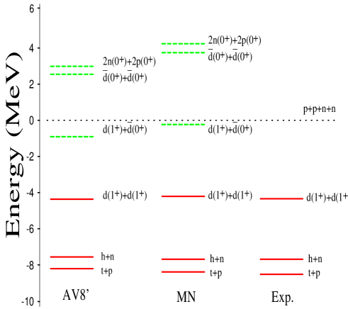
Figure 2: Two-body thresholds calculated with the AV8^′ (left) and MN (middle) potentials. The solid lines are physical channels and the dashed lines are pseudo channels. We also plot experimental two-body thresholds for physical channels (right). The dotted line is the $p$+$p$+$n$+$n$ threshold.

5 Results

5.1 $2N$+$2N$ and $3N$+$N$ channels

In Table 1, we gave the physical channels, $d$+$d$, $t$+$p$, and $h$+$n$. Fig. 2 displays two-body decay thresholds in the $d$+$d$ threshold energy region. The three physical channels are the main channels that describe the scattering around the three lowest thresholds ($d$+$d$, $t$+$p$, $h$+$n$). However, the scattering wave function $\Psi^{JM\pi}_{\rm int}$ in the internal region should contain all effects that may occur when all the nucleons come close to each other. It is thus reasonable that $\Psi^{JM\pi}_{\rm int}$ may not be well described in terms of the physical channels alone. Particularly the deuteron can be easily distorted when we use realistic potentials.

We will show that some pseudo $2N$+$2N$ channels are indeed needed to simulate the distortion of the deuteron. These pseudo channels, when they are included in the phase-shift calculation, are expected to take account of the distortion of the clusters of the entrance channel [30]. Here “pseudo” means that the clusters in the pseudo channels are not physically observable but may play a significant role in the internal region. The wave functions of these $2N$ pseudo clusters are obtained by diagonalizing the intrinsic cluster Hamiltonian similarly to the case of the physical clusters. We take into account the following pseudo clusters: $d^{*}(1^{+},T=0),\ d^{*}(0^{+},T=1),\ d^{*}(2^{+},T=0),\ d^{*}(3^{+},T=0)$, $2n^{*}(0^{+},T=1)$, and $2p^{*}(0^{+},T=1)$, where the upper suffix * indicates all the excited state but the ground state of $d$. Among the pseudo clusters, the lowest energy states with 0⁺ that are related to virtual states would be most important. We especially write them as $\bar{d}(0^{+})$, 2$n(0^{+})$ (di-neutron) and 2$p(0^{+})$ (di-proton). Although they are not bound, they are observed as resonances or quasi-bound states with negative scattering lengths. In fact the scattering lengths are $a_{s}(nn)=-$16.5 fm and $a_{s}(pp)=-$17.9 fm, which are comparable to $a_{s}(np,T=1)=-$23.7 fm. The calculated thresholds of these pseudo channels are also drawn in Fig. 2.

Table 3: $2N$+$2N$ and $3N$+$N$ channels. The Roman and Arabic numerals correspond to sets of channels included in the calculations.

model			channel
	$2N$+$2N$	I	$d(1^{+})$+$d(1^{+})$
			$d(1^{+})$+$d^{*}(1^{+})$
			$d^{*}(1^{+})$+$d^{*}(1^{+})$
		II	$\bar{d}(0^{+})$+$\bar{d}(0^{+})$
			$\bar{d}(0^{+})$+$d^{*}(0^{+})$
			$d^{*}(0^{+})$+$d^{*}(0^{+})$
		III	$d^{*}(2^{+})$+$d^{*}(1^{+})$
			$d^{*}(2^{+})$+$d^{*}(2^{+})$
		IV	$d^{*}(3^{+})$+$d^{*}(1^{+})$
FULL			$d^{*}(3^{+})$+$d^{*}(2^{+})$
			$d^{*}(3^{+})$+$d^{*}(3^{+})$
		V	$2n(0^{+})$+$2p(0^{+})$
			$2n(0^{+})$+$2p^{*}(0^{+})$
			$2n^{*}(0^{+})$+$2p(0^{+})$
			$2n^{*}(0^{+})$+$2p^{*}(0^{+})$
	$3N$+$N$	1	$t(\frac{1}{2}^{+})$+$p(\frac{1}{2}^{+})$
			$t^{*}(\frac{1}{2}^{+})$+$p(\frac{1}{2}^{+})$
		2	$h(\frac{1}{2}^{+})$+$n(\frac{1}{2}^{+})$
			$h^{*}(\frac{1}{2}^{+})$+$n(\frac{1}{2}^{+})$

Though it is expected that the pseudo channels with low threshold energies contribute more strongly to the scattering phase shift, we take into account all of these $2N$+$2N$ channels that include a vanishing total isospin as given in Fig. 2. The total isospin of the $3N$+$N$ channel is mixed in the present calculation. Because the $T$=1 component of the scattering wave function only weakly couples to the $d(1^{+},T=0)$+$d(1^{+},T=0)$ elastic-channel, the channel $d(1^{+},T=0)$+$\bar{d}(0^{+},T=1)$ is not employed in the calculation.

We also include the excited deuteron channels that comprise the $d^{*}(2^{+},T=0)$ and $d^{*}(3^{+},T=0)$ clusters. The energies of these lowest thresholds are above 10 MeV. These channels are therefore expected not to be very important, but that is not always the case as will be discussed in the case of the ¹S₀ $d$+$d$ phase shift.

Table 3 summarizes all the channels that are used in our calculation. The 2$N$+2$N$ channels are distinguished by Roman numerals, while the 3$N$+$N$ channels are labeled by Arabic numerals. In the following, we use an abbreviation “2$N$+2$N$” or “3$N$+$N$” to indicate calculations including all 2$N$+2$N$ channels I-V or all 3$N$+$N$ channels (1-2 in Table 3), respectively. Here $t^{*}(\frac{1}{2}^{+})$ and $h^{*}(\frac{1}{2}^{+})$ are excited 3$N$ continuum states. A “FULL” calculation indicates that all the channels in the table are included to set up the $S$-matrix. In the case of the MN potential channels III and IV are not included because this potential contains no tensor force.

The relative wave functions $\chi_{\alpha m}$ are expanded with 15 basis functions. We checked the stability of the $S$-matrix against the choice of the channel radius. The channel radius employed in this calculation is about 15 fm.

5.2 Positive parity phase shifts

Fig. 3 displays the ${}^{1}S_{0}$ $d$+$d$ elastic-scattering phase shift obtained with the AV8^′ potential. The dash-dotted line is the phase shift calculated with channel I ($I_{d}=1^{+}$), and the dash-dot-dotted line is the phase shift with channels I and II ($I_{d}=1^{+},0^{+}$). The phase shifts calculated by including further excited deuterons are also plotted by the dashed and dotted lines that correspond to the channels I-III ($I_{d}\leq 2^{+}$) and I-IV ($I_{d}\leq 3^{+}$), respectively. A naive expectation that the ${}^{1}S_{0}$ $d$+$d$ elastic-scattering phase shift might be well described in channel I ($d(1^{+})+d(1^{+})$, $d(1^{+})+d^{*}(1^{+})$ and $d^{*}(1^{+})+d^{*}(1^{+})$) alone completely breaks down in the case of the AV8^′ potential.

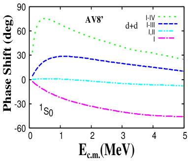
Figure 3: ${}^{1}S_{0}$ $d$+$d$ elastic-scattering phase shift calculated with the AV8^′ potential. The phase shifts are all obtained within the $d$+$d$ channels. The set of included channels is successively increased from I to IV. See Table 3 for the deuteron states included in each channel.

Because the deuteron has a virtual state $\bar{d}$ with $0^{+}$ at low excitation energy, it is reasonable that the inclusion of channel II gives rise to a considerable attractive effect of several tens of degrees on the phase shift, as shown by the dash-dot-dotted line of Fig. 3. However, the phase shift exhibits no converging behavior even when the higher spin states such as $d^{*}$(2⁺) and $d^{*}$(3⁺) are taken into account in the calculation. The additional attractions by these channels are of the same order as that of channel II. One may conclude that the deuteron is strongly distorted even in the low energy ${}^{1}S_{0}$ $d$+$d$ elastic scattering but more physically we have to realize that there exist two observed $0^{+}$ states below the $d$+$d$ threshold. Obviously the $d$+$d$ scattering wave function is subject to the structure of those states in the internal region.

The second 0⁺ state of ⁴He lying about 4 MeV below the $d$+$d$ threshold is known to have a $3N$+$N$ cluster structure [39, 34]. Thus this state together with the ground state of ⁴He cannot be described well in the $2N$+$2N$ model space alone. As seen in Table 1, the $3N$+$N$ channel contains a ${}^{1}S_{0}$ component, which is the dominant component of the $0^{+}_{2}$ state. Since the realistic force strongly couples the $2N$+$2N$ channel to the $3N$+$N$ channel and the $d$+$d$ scattering wave function has to be orthogonal to the main component of the underlying $0^{+}$ states, we expect that the deuteron in the incoming $d$+$d$ channel never remains in its ground state but has to be distorted largely due to the $3N$+$N$ channel. The phase shift for the channel I-IV (dotted line) shows a resonant pattern. This resonant state is expected to be the second 0⁺ state because of the restricted model space within the $d$+$d$ channel.

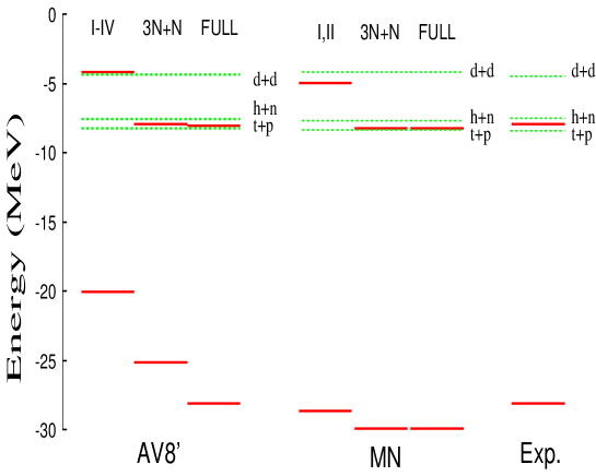
Figure 4: Comparison of the ground and second 0⁺ state energies between calculations with the AV8^′ (left) and MN (middle) potentials and experiment (right). The model space for AV8^′ is I-IV, $3N$+$N$ and FULL and the model space for MN is I-II, $3N$+$N$ and FULL.

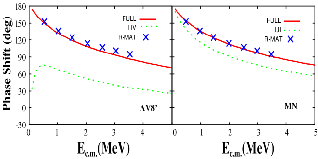
Figure 5: ${}^{1}S_{0}$ $d$+$d$ elastic-scattering phase shift calculated with the AV8^′ (left) and MN (right) potentials. The solid line is a FULL calculation, while the dotted line is a $d$+$d$ channel calculation. Crosses correspond to the $R$-matrix analysis of Ref. [22].

Fig. 4 displays the calculated ground state energy and the second 0⁺ energy for the AV8^′ (left) and MN (middle) potentials. The model spaces of the calculations are I-IV, $3N$+$N$ and FULL for AV8^′ and I-II, $3N$+$N$ and FULL for MN. We also plot experimental energies (right) [40]. For the AV8^′ potential, the energies of the two lowest $0^{+}$ states do not change very much between the FULL and $3N$+$N$ models. But the second 0⁺ state with the $d$+$d$ model (channels I-IV) is not bound with respect to the $d$+$d$ threshold as expected before. On the contrary, for the MN potential, the second 0⁺ state with the $d$+$d$ model (channels I-II) is bound with respect to the $d$+$d$ threshold. We consider that this difference makes the drastic change of the $d$+$d$ phase shifts, between the AV8^′ and MN potentials. It is also interesting to see that the energies of the two lowest $0^{+}$ states for the MN potential are almost the same between the FULL and $3N$+$N$ models.

Plotted in Fig. 5 are the ${}^{1}S_{0}$ $d$+$d$ elastic-scattering phase shifts obtained with the AV8^′ potential (left) and the MN potential (right). The FULL calculation (solid line) couples all 2$N$+2$N$ and 3$N$+$N$ channels that are listed in Table 3. The $R$-matrix analysis (crosses) [22] is reproduced well by both the AV8^′ and MN potential with the FULL calculation. Compared to the uncoupled phase shift (dotted line), one clearly sees that the 3$N$+$N$ channel produces a very large effect on the $d$+$d$ elastic phase shift, especially in the case of the AV8^′ potential. We also verified that a calculation excluding the channels III, IV or V from the FULL channel calculation gives only negligible change in the phase shift. The slow convergence seen in Fig. 3 is thus attributed to the neglect of the $3N$+$N$ channel, indicating that a proper account of the ${}^{1}S_{0}$ $d$+$d$ elastic phase shift at low energy can be possible only when the coupled channels {$d$(1⁺)+$d$(1⁺)} +{$d$(0⁺)+$d$(0⁺)}+ {$t$(1/2⁺)+$p(1/2^{+})$} +{$h$(1/2⁺)+$n(1/2^{+})$} are considered.

Thus, the slow convergence in Fig. 3 suggests that the $2N$+$2N$ partition is not an economical way to include the effects of the $3N$+$N$ channel. In the case of the MN potential (right panel in Fig. 5), the situation is very different from the AV8^′ case. The channel coupling effect is rather modest, and the size of the ${}^{1}S_{0}$ $d$+$d$ elastic phase shift is already accounted for mostly in the $d$+$d$ channel calculation. All these results are very consistent with the $0^{+}$ spectrum in Fig. 4.

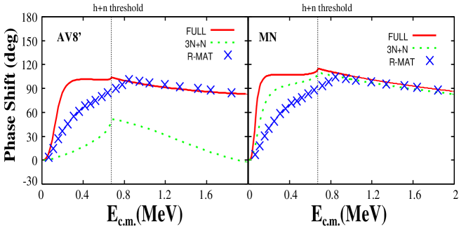
Figure 6: ${}^{1}S_{0}$ $t$+$p$ elastic-scattering phase shift at energies below the $d$+$d$ threshold. The solid line is a FULL calculation, while the dashed line is a $3N$+$N$ channel calculation. Crosses correspond to the $R$-matrix analysis of Ref. [22].

The large distortion effect of the deuteron clusters on the ${}^{1}S_{0}$ $d$+$d$ scattering phase shift is expected to appear in the 3$N$+$N$ phase shift as well because of the coupling between the 3$N$+$N$ and 2$N$+2$N$ channels. We display in Fig. 6 the ${}^{1}S_{0}$ $t$+$p$ elastic-scattering phase shift at energies below the $d$+$d$ threshold. The 0${}^{+}_{2}$ state of ⁴He is observed as a sharp resonance with a proton decay width of 0.5 MeV at about 0.4 MeV above the $t$+$p$ threshold. The present energies ($E_{r}=0.15$ MeV for AV8^′, $E_{r}=0.12$ MeV for MN) calculated with a bound state approximation are slightly smaller than the experimental value, but they are consistent with a calculation ($E_{r}=0.105$ MeV and $\Gamma/2=0.129$ MeV for AV18+UIX, $E_{r}=0.091$ MeV and $\Gamma/2=0.077$ MeV for AV18+UIX+V${}^{*}_{3}$) with another realistic interaction (AV18) with three nucleon forces by Hofmann and Hale [22]. The calculated phase shifts appear slightly larger than that in the $R$-matrix analysis (crosses in Fig. 6) [22]. It is noted that the phase shift changes so much even for a small change of the 0${}^{+}_{2}$ resonant pole position ($\sim$0.1 MeV) because it is very near to the threshold. The phase shifts in the FULL calculation, for both AV8^′ and MN cases, show a resonance pattern in a small energy interval and the overall energy dependencies of the phase shifts are similar to each other. However, the phase shifts obtained only in the $3N$+$N$ channel are quite different as indicated by the dotted lines in Fig. 6. In the case of the MN potential (right) the phase shift is already close to the FULL phase shift, while in the case of the AV8^′ potential (left) the phase shift is much smaller (by almost 90 degrees) and moreover shows no resonance pattern.

By looking into the wave functions in more detail, we argue that the large distortion effect in the ${}^{1}S_{0}$ $d$+$d$ and $3N$+$N$ coupled channels is really brought about by the tensor force. As shown in Table  2, the AV8^′ potential with TNF gives 5.8% and 8.4% (8.3%) $D$-state probability for $d$ and $t$ $(h)$, respectively. Thus the $d$+$d$ state in the ${}^{1}S_{0}$ state contains $L=S=0$ components (89%) as well as $L=S=2$ components (11%), where $L$ and $S$ are the total orbital and spin angular momenta of the four-nucleon system. Similarly the $3N$+$N$ state in the ${}^{1}S_{0}$ state contains an $L=S=0$ component (92%) and an $L=S=2$ component (8%). Thus the tensor force couples both states with $\Delta L=2$ and $\Delta S=2$ couplings, which are in fact very large compared to the central matrix element ($\Delta L=0$, $\Delta S=0$). An analysis of this type was performed for some levels of ⁴He in Refs. [7, 39]. The MN potential contains no tensor force, so that the $d$+$d$ and $3N$+$N$ channel coupling is modest.

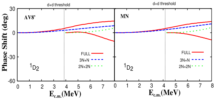
Figure 7: ${}^{1}D_{2}$ elastic-scattering phase shifts with the AV8^′ (left) and MN (right) potentials. The model space for the solid line is FULL. The $t$+$p$ phase shift starts from the $t$+$p$ zero energy and the $d$+$d$ phase shift starts from the $d$+$d$ threshold. The dashed line is the $t$+$p$ phase shift with only the 3$N$+$N$ channel and the dotted line is the $d$+$d$ phase shift with only the 2$N$+2$N$ channel.

As listed in Table 1, there are four channels, ${}^{5}S_{2}$, ${}^{1}D_{2}$, ${}^{3}D_{2}$ and ${}^{5}D_{2}$, for $J^{\pi}=2^{+}$ at energies around the $d$+$d$ threshold. Among these states, we expect that the effect of the coupling between the 3$N$+$N$ and 2$N$+2$N$ channels occurs most strongly in ${}^{1}D_{2}$ as it appears in all physical channels. However, no sharp resonance is observed in ⁴He up to 28 MeV of excitation energy, so that the coupling effect, if any, might be weaker than that observed in the ${}^{1}S_{0}$ case.

Fig. 7 displays the ${}^{1}D_{2}$ elastic-scattering phase shifts obtained in three types of calculations, $3N$+$N$ (dashed line), $2N$+$2N$ (dotted line), and FULL (solid line). The $t$+$p$ and $d$+$d$ phase shifts start from the $t$+$p$ ($E_{\rm c.m.}=0$) and $d$+$d$ thresholds, respectively. The phase shifts of the $3N$+$N$ and $2N$+$2N$ calculations are both slightly positive, indicating a weak attraction in the $t$+$p$ and $d$+$d$ interactions. In the FULL calculation, the $t$+$p$ phase shift becomes more attractive and the $d$+$d$ phase shift turns to be negative (repulsive). The present FULL calculation reproduces the calculation of Ref. [22] as expected. Though the effect of the coupling is slightly larger in the AV8^′ potential than in the MN potential, it is much less compared to the case of the ${}^{1}S_{0}$ phase shift. This is understood as follows. In the ${}^{1}D_{2}$ state, the main component of the wave function is given by the $L=2$, $S=0$ state: Its probability is the same as that of ${}^{1}S_{0}$, that is, 92% in $t$+$p$ and 89% in $d$+$d$. However, the probability of finding the state with $L=0$, $S=2$, which causes a strong tensor coupling, is more than one order of magnitude smaller than in the case of ${}^{1}S_{0}$, namely 0.23% in $t$+$p$ and 0.44% in $d$+$d$, respectively. The reason for this small percentage is that, to obtain $L=0$, the incoming $D$-wave in the ${}^{1}D_{2}$ channel must couple with the $D$-components in the clusters, but this coupling leads to several fragmented components with different $L$ values. This relatively weaker coupling of the tensor force explains the phase shift behavior in Fig. 7.

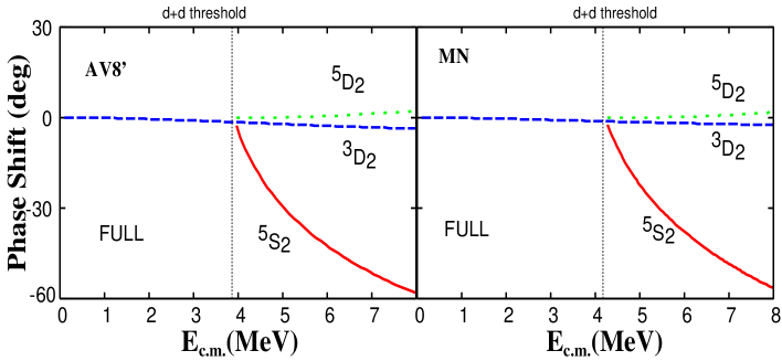
Figure 8: Elastic scattering phase shifts of the 2⁺ state obtained in a FULL calculation with the AV8^′ (left) and MN (right) potentials. Solid line: ${}^{5}S_{2}$ $d$+$d$ phase shift, dotted line: ${}^{5}D_{2}$ $d$+$d$ phase shift, dashed line: ${}^{3}D_{2}$ $t$+$p$ phase shift.

In Fig. 8 we plot the $t$+$p$ and $d$+$d$ elastic-scattering phase shifts for other channels, ${}^{5}S_{2}$ (solid line), ${}^{3}D_{2}$ (dashed line), and ${}^{5}D_{2}$ (dotted line). We show only the FULL result, because the phase shifts with the truncated basis do not change visibly at the scale of the figure. The obtained phase shifts are not that different between the AV8^′ and MN potentials, and also consistent with the previous calculation [22]. Thus, the effect of the distortion of the clusters is very small for 2⁺ except for ${}^{1}D_{2}$.

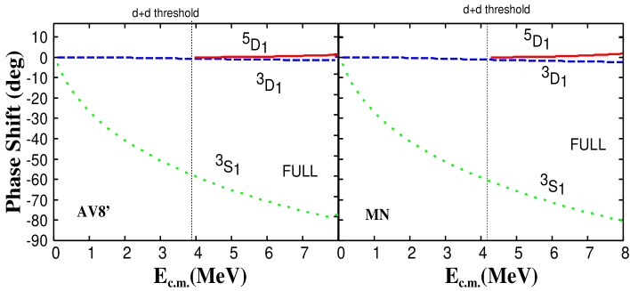
Figure 9: Elastic scattering phase shifts of the 1⁺ state in a FULL calculation with the AV8^′ (left) and MN (right) potentials. Solid line: ${}^{5}D_{1}$ $d$+$d$ phase shift, dotted line: ${}^{3}S_{1}$ $t$+$p$ phase shift, dashed line: ${}^{3}D_{1}$ $t$+$p$ phase shift.

We have three channels for $J^{\pi}=1^{+}$, ${}^{5}D_{1}$, ${}^{3}D_{1}$ and ${}^{3}S_{1}$. No sharp $1^{+}$ resonance of ⁴He is observed experimentally up to 28  MeV of excitation energy. Another theoretical calculation neither predicts it [39], so that the coupling between the 2$N$+2$N$ and 3$N$+$N$ channels is expected to be weak. Fig. 9 exhibits the $t$+$p$ and $d$+$d$ elastic-scattering phase shifts in the FULL calculation: ${}^{5}D_{1}$ $d$+$d$ (solid line), ${}^{3}D_{1}$ $t$+$p$ (dashed line), and ${}^{3}S_{1}$ $t$+$p$ (dotted line). Only the FULL result is displayed because the phase shift change in other calculations is small. Both AV8^′ and MN potentials produce phase shifts quite similar to each other.

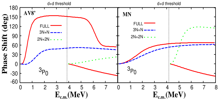
Figure 10: ${}^{3}P_{0}$ elastic-scattering phase shifts calculated with the AV8^′ (left) and MN (right) potentials. See the caption of Fig. 7.

5.3 Negative parity phase shifts

As seen from Table 1, the main components of these negative parity states are considered to be ${}^{3}P_{J}$.

We compare in Fig. 10 the ${}^{3}P_{0}$ elastic-scattering phase shifts calculated with the AV8^′ (left) and MN (right) potentials. The truncated $3N$+$N$ (dashed line) and $2N$+$2N$ (dotted line) calculations are shown together with the FULL result (solid line). The $t$+$p$ phase shift of the $3N$+$N$ calculation is similar with both AV8^′ and MN potentials, while the $d$+$d$ phase shift of the $2N$+$2N$ calculation behaves quite differently between the two potentials: the $d$+$d$ phase shift is weakly attractive with AV8^′ but is very strongly attractive with MN. No typical resonance behavior shows up below the $d$+$d$ threshold, which is in contradiction to experiment. In the FULL model that combines both 3$N$+$N$ and 2$N$+2$N$ configurations, however, the two potentials predict quite different phase shifts especially in the $t$+$p$ channel. The $t$+$p$ phase shift with AV8^′ becomes so attractive that it crosses $\pi/2$, indicating a resonance at about 1 MeV above the $t$+$p$ threshold. The $d$+$d$ phase shift changes sign from attractive to repulsive. The result based on the AV8^′ potential is thus consistent with experiment. Furthermore, we reproduce the flat structure of the ${}^{3}P_{0}$ phase shift around several MeV above the $t$+$p$ threshold which was discussed as the coupling to the $h$+$n$ channel [22]. On the other hand, the MN potential changes the $t$+$p$ phase shift only mildly and produces no sharp resonance behavior. The $d$+$d$ phase shift changes drastically to the repulsive side.

As seen in the above figure, the sharp 0^- state appears provided a full model space with a realistic potential is employed. The mechanism to produce this resonance is unambiguously attributed to the tensor force as discussed in Ref. [7] for the realistic interaction G3RS [41]. According to it, the $0^{-}$ state consists of only two components, $L=S=1$ (95.5%) and $L=S=2$ (4.5%), ignoring a tiny component with $L=S=0$. The $L=S=2$ component arises from the coupling of the incoming $P$-wave with the $D$-states contained in the $3N$ and $d$ clusters. All the pieces of the Hamiltonian but the tensor force have no coupling matrix element between the two components. The uncoupled Hamiltonian thus gives a too high energy to accommodate a resonance. The tensor force, however, couples the two components very strongly, bringing down its energy to a right position.

The second lowest negative parity state has spin-parity 2^-. The physical channel for this state is only ${}^{3}P_{2}$ as seen in Table 1. Fig. 11 compares the ${}^{3}P_{2}$ elastic-scattering phase shifts in a manner similar to Fig. 10. The phase shift obtained with the MN potential is almost the same as the ${}^{3}P_{0}$ phase shift, which is consistent with the previous result [39] that the energies of the negative parity states calculated with the MN potential are found to be degenerate. In the case of the AV8^′ potential, the ${}^{3}P_{2}$ phase shifts grows significantly in the FULL calculation, indicating a resonant behavior. The coupling effect between the $3N$+$N$ and $2N$+$2N$ channels is however much less compared to the $0^{-}$ state. This is because the incoming $P$-wave coupled to the $D$-states in the clusters gives rise to several $L$ values to produce the $2^{-}$ state and therefore the tensor coupling does not concentrate sufficiently to produce a sharp resonance.

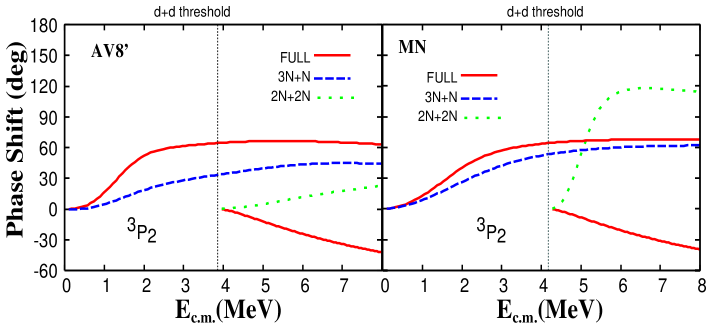
Figure 11: ${}^{3}P_{2}$ elastic-scattering phase shifts calculated with the AV8^′ (left) and MN (right) potentials. See the caption of Fig. 7.

Fig. 12 displays the ${}^{3}P_{1}$ and ${}^{1}P_{1}$ elastic-scattering phase shifts calculated with the AV8^′ (left) and MN (right) potentials. Note that no physical $d$+$d$ channel exists in the case of the ${}^{1}P_{1}$ state. Because both FULL and $3N$+$N$ calculations give almost the same phase shifts, only the FULL result is shown in the figure. The ${}^{3}P_{1}$ phase shift calculated with the MN potential is again almost the same as those of the ${}^{3}P_{0}$ and ${}^{3}P_{2}$ cases, supporting that the three negative parity states become almost degenerate. The ${}^{3}P_{1}$ elastic-scattering phase shift calculated with the AV8^′ potential is qualitatively similar to that of ${}^{3}P_{2}$. The attractive nature of the $t$+$p$ phase shift becomes further weaker, and to identify a resonance appears to be very hard. Even though it is possible in some way, its width would be a few MeV, which is not in contradiction to experiment. The ${}^{1}P_{1}$ phase shifts are very small in both AV8^′ and MN cases.

For the negative parity states, the FULL model with the AV8^′ potential gives results that are consistent with both experiment and the theoretical calculation of Ref. [39]. We have pointed out that the phase shift behavior reveals the importance of the tensor force particularly in the case of $0^{-}$. Its effect is often masked however by the coupling between the $D$ states in the clusters and the incoming partial wave.

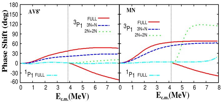
Figure 12: ${}^{3}P_{1}$ and ${}^{1}P_{1}$ elastic-scattering phase shifts calculated with the AV8^′ (left) and MN (right) potentials. See the caption of Fig. 7.

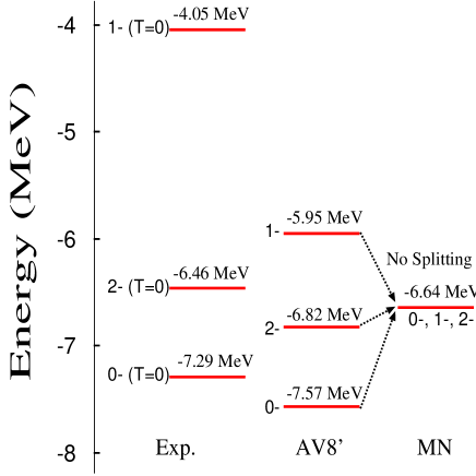
Figure 13: Comparison of energies with respect to the four-nucleon threshold for negative parity states (0^-, 1^-, 2^-) between the experiment (left), AV8^′ (middle) and MN (right).

In this subsection, we investigate the phase shifts of the negative parity states which have dominant $T=0$ components. In Fig. 13, we represent three experimental negative parity $T=0$ energies (left). The states are observed at $-7.29$ ($0^{-}$), $-6.46$ ($2^{-}$) and $-4.05$ ($1^{-}$) MeV below the four-nucleon threshold [40]. The former two are located below the $d$+$d$ threshold and their widths are 0.84 and 2.01 MeV, respectively, whereas the last one is above the $d$+$d$ threshold and its width is fairly broad (6.1 MeV). Here, we calculate these energies as $-7.57$ ($0^{-}$), $-6.82$ ($2^{-}$) and $-5.95$ ($1^{-}$) MeV, which are approximated by the half-value position from the maximum phase shifts. The present calculation is not projected out to $T=0$, but the dominant configurations of $t$+$p$, $h$+$n$ and $d$+$d$ elastic scattering are $T=0$. Our calculated energies with AV8^′ reproduce the ordering of $0^{-}$, $2^{-}$ and $1^{-}$ (middle in Fig. 13). The splitting between the two lower states $0^{-}$ and $2-$ is reproduced, but the experimental $1^{-}$ energy is higher than the calculation. However, the determination of the energy for such a high energy state with large decay width (6.1 MeV) is very difficult from both experimental and theoretical side, and it usually has a large ambiguity.

This type of analysis was done by Horiuchi and Suzuki, who applied the correlated Gaussian basis with two global vectors to study the energy spectrum of ⁴He [39]. Because the results of Ref. [39] are based on approximate solutions that impose no proper resonance boundary condition, it is interesting to see how the tensor force changes the phase shifts in the negative parity states as shown in this subsection. These authors also found that the negative parity states with $T=0$ turn out to be almost degenerate when the MN potential that contains no tensor force is employed. In the present calculation, three states ($0^{-}$, $1^{-}$, $2^{-}$) completely degenerate at the same energy, $E=-6.64$ MeV (right), and the same phase shift pattern (solid lines in Figs. 10, 11, 12). Thus we can expect to see a clear evidence for the tensor force in the scattering involving the negative parity states.

6 Summary and conclusion

We have investigated the distortion of clusters appearing in the low-energy $d$+$d$ and $t$+$p$ elastic scattering using a microscopic cluster model with the triple global vector method. We showed that the tensor interaction changes the phase shifts very much by comparing a realistic interaction and an effective interaction. In the present $ab$-$initio$ type cluster model, the description of the cluster wave functions is extended from a simple (0$s$) harmonic-oscillator shell model to a few-body model. To compare distortion effects of the clusters with realistic and effective interactions, we employed the AV8^′ potential as a realistic interaction and the MN potential as an effective interaction.

For the realistic interaction, the calculated ${}^{1}S_{0}$ phase shift shows that the $t$+$p$ and $h$+$n$ channels strongly couple with the $d$+$d$ channel. These channels are coupled because of the tensor interaction. On the contrary, the coupling of these $3N$+$N$ channels plays a relatively minor role for the case of the effective interaction because of the absence of tensor term. In other words, the $3N$+$N$ channels strongly affect the $d$+$d$ elastic phase shift with the realistic interaction, but not with the effective interaction.

For the 2⁺ phase shifts, there is a ${}^{1}D_{2}$ component in all physical channels ($d$+$d$, $t$+$p$ and $h$+$n$). The coupling of the $2N$+$2N$ and $3N$+$N$ channels in ${}^{5}D_{2}$ is weaker than in ${}^{1}S_{2}$ because of a weaker tensor coupling as discussed in section 5, and the calculated phase shifts are very similar for the realistic and effective potentials. For other positive parity cases, the phase shift behavior of the realistic and effective potentials are very similar, and the coupling between the $2N$+$2N$ and $3N$+$N$ channels can be neglected or is very small. Furthermore, the tensor interaction makes the energy splitting of the $0^{-}$, $2^{-}$ and $1^{-}$ negative parity states of ⁴He consistent with experiment. No such splitting is however reproduced with the effective interaction.

We believe that the physical picture obtained in the large model space with the realistic interaction should be close to the real physical situation. It is needless to say that $ab$-$initio$ reaction calculations are very important to understand the underlying reaction dynamics involving continuum states. Simpler calculations using effective interactions in the same framework, as carried out in the present paper, are also meaningful because we can understand more clearly the effect of the tensor force by comparing both calculations. The reaction calculations with the microscopic cluster model, whose model space and interactions are restricted, have been successfully applied to many heavier nuclei. Therefore, it is instructive to see the difference from the realistic interaction by employing a simple conventional effective interaction as MN in the few-nucleon systems.

It will be quite interesting to see the importance of the tensor force in reaction observables of four nucleons. As a direct application of the present study the radiative capture reaction $d(d,\gamma)^{4}$He at energies of astrophysical interest is of prime importance. It is expected to take place predominantly via $E2$ transitions [42, 27, 43, 20, 9]. As is seen from Table 1, the two deuterons can approach each other in the $S$-wave only when $J^{\pi}$ is either 0⁺ (${}^{1}S_{0}$) or 2⁺ (${}^{5}S_{2}$). The former case is excluded because a radiative capture reaction of $0^{+}\to 0^{+}$ is forbidden in the lowest-order electromagnetic interaction, and hence the $E2$ transition should be predominant. If there were no tensor force present, the radiative capture would be suppressed near $E=0$ because neither $d$ nor ⁴He would have a $D$-wave component in contradiction with the flat behavior of the astrophysical $S$-factor [44]. The tensor force strongly changes this story because it can couple $S$- and $D$-waves, bringing a significant amount of $D$-state probability in both ⁴He and $d$. Details of this analysis will be reported elsewhere.

Acknowledgment
We thank Dr. R. Kamouni for helpful discussions based on his PhD thesis (in French). This work presents research results of Bilateral Joint Research Projects of the JSPS (Japan) and the FNRS (Belgium). Y. S. is supported by a Grant-in-Aid for Scientific Research (No. 21540261). This text presents research results of the Belgian program P6/23 on interuniversity attraction poles initiated by the Belgian-state Federal Services for Scientific, Technical and Cultural Affairs (FSTC). D. B. and P. D. also acknowledge travel support of the Fonds de la Recherche Scientifique Collective (FRSC). The part of computational calculations were carried out in T2K-Tsukuba.

Appendix A Definitions of recoupling coefficients

We define an auxiliary coefficient $Z$ that appears in the coupling

$$[[Y_{a}({\mbox{\boldmath$e$}}_{1})[Y_{b}({\mbox{\boldmath$e$}}_{1})Y_{b}({\mbox{\boldmath$e$}}_{2})]_{0}]_{a}\to Z(ab)[Y_{a+b}({\mbox{\boldmath$e$}}_{1})Y_{b}({\mbox{\boldmath$e$}}_{2})]_{a}.$$ (76)

By introducing a coefficient

$$C(ab,c)=\sqrt{\frac{(2a+1)(2b+1)}{4\pi(2c+1)}}\langle a\ 0\ b\ 0|c\ 0\rangle\\$$ (77)

for the coupling $[Y_{a}({\mbox{\boldmath$e$}}_{1})Y_{b}({\mbox{\boldmath$e$}}_{1})]_{c}=C(ab,c)Y_{c}({\mbox{\boldmath$e$}}_{1})$, we can express $Z$ as

$$Z(ab)=\sqrt{\frac{2(a+b)+1}{(2a+1)(2b+1)}}C(ab,a+b)=\frac{1}{\sqrt{4\pi}}\langle a\ 0\ b\ 0|a+b\ 0\rangle.$$ (78)

Note that $C(ab,c)$ vanishes unless $a+b+c$ is even.

The coefficients that appear in Sect. 4 are given as follows:

$${}X(a\ b\ c)=Z(ab)Z(ac)C(bc,b+c)U(a\!+\!c\ c\ a\!+\!b\ b;\ a\ b\!+\!c),$$ (79)

$${}R_{3}(a\ b\ c)=Z(ab)Z(a\!+\!b\ c),$$ (80)

$${}W(a\ b\ c\ q\ Q,\ a^{\prime}\ b^{\prime}\ c^{\prime}\ q^{\prime}\ Q^{\prime},\ \ell\ \ell^{\prime})$$

$${}=\left[\begin{array}[]{ccc}q&c&Q\\ q^{\prime}&c^{\prime}&Q^{\prime}\\ \ell^{\prime}&c\!+\!c^{\prime}&\ell\\ \end{array}\right]\left[\begin{array}[]{ccc}a&b&q\\ a^{\prime}&b^{\prime}&q^{\prime}\\ a\!+\!a^{\prime}&b\!+\!b^{\prime}&\ell^{\prime}\\ \end{array}\right]C(aa^{\prime},a\!+\!a^{\prime})C(bb^{\prime},b\!+\!b^{\prime})C(cc^{\prime},c\!+\!c^{\prime}).$$ (87)

Appendix B Matrix elements for various operators

The purpose of this appendix is to collect formulas for various matrix elements. The main procedure to derive the formulas is sketched in Sect. 4. More details for the case of two global vectors are given in Ref. [7].

B.1 Kinetic energy

Let ${\mbox{\boldmath$\pi$}}_{j}$ denote the momentum operator conjugate to ${\mbox{\boldmath$x$}}_{j}$, ${\mbox{\boldmath$\pi$}}_{j}=-i\hbar\frac{\partial}{\partial{\mbox{\boldmath$x$}}_{j}}$. The total kinetic energy operator for the $N$-nucleon system with its center of mass kinetic energy being subtracted takes the form

$$\sum_{i=1}^{N}\frac{{\mbox{\boldmath$p$}}_{i}^{2}}{2m}-\frac{{\mbox{\boldmath$\pi$}}_{N}^{2}}{2Nm}=\frac{1}{2}\widetilde{\mbox{\boldmath$\pi$}}\Lambda{\mbox{\boldmath$\pi$}},$$ (88)

where ${\mbox{\boldmath$\pi$}}_{N}=\sum_{i=1}^{N}{\mbox{\boldmath$p$}}_{i}$ is the total momentum, $\widetilde{\mbox{\boldmath$\pi$}}=({\mbox{\boldmath$\pi$}}_{1},{\mbox{\boldmath$\pi$}}_{2},\ldots,{\mbox{\boldmath$\pi$}}_{N-1})$, and $\Lambda$ is an $(N-1)\times(N-1)$ symmetric mass matrix. Defining $N-1$-dimensional column vectors $\Gamma_{i}$ as

$$\Gamma_{i}=A^{\prime}B^{-1}u_{i}\ \ \ \ \ \ (i=1,2,3),$$

$$\Gamma_{i}=-AB^{-1}u_{i}\ \ \ \ \ (i=4,5,6)$$ (89)

and an $(N-1)\times(N-1)$ matrix $Q$

$$Q_{ij}=2\widetilde{\Gamma_{i}}\Lambda\Gamma_{j},$$ (90)

we can calculate the matrix element for the kinetic energy through the overlap matrix element

$$\langle F^{\prime}|\frac{1}{2}\widetilde{\mbox{\boldmath$\pi$}}\Lambda{\mbox{\boldmath$\pi$}}|F\rangle=\frac{\hbar^{2}}{2}\left(R-\sum_{i<j}Q_{ij}\frac{\partial}{\partial\rho_{ij}}\right)\left<F^{\prime}|F\right>,$$ (91)

where

$$R=3{\rm Tr}(B^{-1}A^{\prime}\Lambda A).$$ (92)

The $\rho_{ij}$ values are defined in Eq. (60).

B.2 $\delta$-function

A two-body interaction $V({\mbox{\boldmath$r$}}_{i}-{\mbox{\boldmath$r$}}_{j})$ can be expressed as

$$V({\mbox{\boldmath$r$}}_{i}-{\mbox{\boldmath$r$}}_{j})=\int d{\mbox{\boldmath$r$}}V({\mbox{\boldmath$r$}})\ \delta({\mbox{\boldmath$r$}}_{i}-{\mbox{\boldmath$r$}}_{j}-{\mbox{\boldmath$r$}}).$$ (93)

Once the matrix element of $\delta({\mbox{\boldmath$r$}}_{i}-{\mbox{\boldmath$r$}}_{j}-{\mbox{\boldmath$r$}})$ is obtained, the matrix element of the interaction is calculated by integrating over $r$ the $\delta$-function matrix element weighted with the form factor $V({\mbox{\boldmath$r$}})$. Similarly, for a one-body operator

$$D({\mbox{\boldmath$r$}}_{i}-{\mbox{\boldmath$x$}}_{N})=\int d{\mbox{\boldmath$r$}}D({\mbox{\boldmath$r$}})\ \delta({\mbox{\boldmath$r$}}_{i}-{\mbox{\boldmath$x$}}_{N}-{\mbox{\boldmath$r$}}),$$ (94)

its matrix element can be obtained from that of the $\delta$-function. Because both ${\mbox{\boldmath$r$}}_{i}-{\mbox{\boldmath$r$}}_{j}$ and ${\mbox{\boldmath$r$}}_{i}-{\mbox{\boldmath$x$}}_{N}$ can be expressed in terms of a linear combination of the relative coordinate ${\mbox{\boldmath$x$}}_{i}$, it is enough to calculate the matrix element of $\delta(\widetilde{w}{\mbox{\boldmath$x$}}-{\mbox{\boldmath$r$}})$, where $\widetilde{w}=(w_{1},w_{2},\ldots,w_{N-1})$ is a combination constant to express ${\mbox{\boldmath$r$}}_{i}-{\mbox{\boldmath$r$}}_{j}$ or ${\mbox{\boldmath$r$}}_{i}-{\mbox{\boldmath$x$}}_{N}$.

The matrix element of the $\delta$-function is given by

$${}\left<F^{\prime}|\delta(\widetilde{w}{\mbox{\boldmath$x$}}-{\mbox{\boldmath$r$}})|F\right>$$ (95)

$$= \left(\frac{(2\pi)^{N-1}}{\mbox{det}B}\right)^{3/2}\left(\prod_{i=1}^{6}B_{L_{i}}\right)\frac{(-1)^{L_{1}+L_{2}+L_{3}}\sqrt{2L+1}}{\sqrt{2L^{\prime}+1}}\ \left(\frac{c}{2\pi}\right)^{3/2}{\rm e}^{-\frac{1}{2}cr^{2}}$$

$$\times \sum_{\kappa\mu}\langle LM\kappa\mu|L^{\prime}M^{\prime}\rangle Y_{\kappa\mu}^{*}(\widehat{\mbox{\boldmath$r$}})\sum_{p_{i}}\left(\prod_{i=1}^{6}(-c\gamma_{i}r)^{p_{i}}\frac{\sqrt{2p_{i}+1}}{B_{p_{i}}}\right)$$

$$\times \sum_{\ell_{12}\ell_{45}\ell\ell^{\prime}\overline{L}_{12}\overline{L}_{45}\overline{L}}\frac{(-1)^{\ell+\ell^{\prime}}}{\sqrt{(2\ell+1)(2\overline{L}+1)}}U(L\overline{L}\kappa\ell^{\prime};\ell L^{\prime})\ \overline{O}(p_{i};\ell_{12}\ell_{45}\ell\ell^{\prime}\kappa)$$

$$\times W(p_{1}p_{2}p_{3}\ell_{12}\ell,L_{1}\!-\!p_{1}\ L_{2}\!-\!p_{2}\ L_{3}\!-\!p_{3}\ \overline{L}_{12}\overline{L},LL_{12})$$

$$\times W(p_{4}p_{5}p_{6}\ell_{45}\ell^{\prime},L_{4}\!-\!p_{4}\ L_{5}\!-\!p_{5}\ L_{6}\!-\!p_{6}\ \overline{L}_{45}\overline{L},L^{\prime}L_{45})$$

$$\times \sum_{n_{ij}}\left(\prod_{i<j}^{6}(-\overline{\rho}_{ij})^{n_{ij}}\frac{\sqrt{2n_{ij}+1}}{B_{n_{ij}}}\right)$$

$$\times O(n_{ij};L_{1}\!-\!p_{1}\ L_{2}\!-\!p_{2}\ L_{3}\!-\!p_{3}\ L_{4}\!-\!p_{4},L_{5}\!-\!p_{5}\ L_{6}\!-\!p_{6},\overline{L}_{12}\overline{L}_{45}\overline{L}),$$

with

$$c=(\widetilde{w}B^{-1}w)^{-1},\ \ \ \ \ \gamma_{i}=\widetilde{w}B^{-1}u_{i},\ \ \ \ \ \overline{\rho}_{ij}=\rho_{ij}-c\gamma_{i}\gamma_{j}.$$ (96)

The summation over non-negative integers $n_{ij}$ and $p_{i}$ is restricted by the following equations

$$n_{12}+n_{13}+n_{14}+n_{15}+n_{16}+p_{1}=L_{1},$$

$$n_{12}+n_{23}+n_{24}+n_{25}+n_{26}+p_{2}=L_{2},$$

$$n_{13}+n_{23}+n_{34}+n_{35}+n_{36}+p_{3}=L_{3},$$

$$n_{14}+n_{24}+n_{34}+n_{45}+n_{46}+p_{4}=L_{4},$$

$$n_{15}+n_{25}+n_{35}+n_{45}+n_{56}+p_{5}=L_{5},$$

$$n_{16}+n_{26}+n_{36}+n_{46}+n_{56}+p_{6}=L_{6}.$$ (97)

Here $\overline{O}(p_{i};\ell_{12}\ell_{45}\ell\ell^{\prime}\kappa)$ is defined as a coefficient that appears in the coupling of a product of six terms

$${}\prod_{i=1}^{6}[Y_{p_{i}}({\mbox{\boldmath$e$}}_{i})Y_{p_{i}}(\widehat{\mbox{\boldmath$r$}})]_{00}=\sum_{\ell_{12}\ell_{45}\ell\ell^{\prime}\kappa}\overline{O}(p_{i};\ell_{12}\ell_{45}\ell\ell^{\prime}\kappa)$$ (98)

$$\times [[[[Y_{p_{1}}({\mbox{\boldmath$e$}}_{1})Y_{p_{2}}({\mbox{\boldmath$e$}}_{2})]_{\ell_{12}}Y_{p_{3}}({\mbox{\boldmath$e$}}_{3})]_{\ell}\ [[Y_{p_{4}}({\mbox{\boldmath$e$}}_{4})Y_{p_{5}}({\mbox{\boldmath$e$}}_{5})]_{\ell_{45}}Y_{p_{6}}({\mbox{\boldmath$e$}}_{6})]_{\ell^{\prime}}]_{\kappa}\ Y_{\kappa}(\widehat{\mbox{\boldmath$r$}})]_{00},$$

and it is given by

$$\overline{O}(p_{i};\ell_{12}\ell_{45}\ell\ell^{\prime}\kappa)$$

$$\quad=\sqrt{\frac{2\kappa+1}{\prod_{i=1}^{6}(2p_{i}+1)}}C(p_{1}p_{2},\ell_{12})C(\ell_{12}p_{3},\ell)C(p_{4}p_{5},\ell_{45})C(\ell_{45}p_{6},\ell^{\prime})C(\ell\ell^{\prime},\kappa).$$ (99)

The $r$-dependence of the matrix element (95) is

$${\rm e}^{-\frac{1}{2}cr^{2}}r^{p_{1}+p_{2}+p_{3}+p_{4}+p_{5}+p_{6}}Y_{\kappa\mu}^{*}(\widehat{\mbox{\boldmath$r$}}).$$ (100)

For a central interaction, $V({\mbox{\boldmath$r$}})$ is a scalar function, and the sum over $\kappa$ in Eq. (95) is limited to 0. For a tensor interaction, the angular dependence of $V({\mbox{\boldmath$r$}})$ is proportional to $Y_{2}(\hat{\mbox{\boldmath$r$}})$, and $\kappa$ is limited to 2. The electric multipole operator is a special case of one-body operator, so that one can make use of the formula (95) to calculate its matrix element. More explicitly, we give the matrix element of $V(|\widetilde{w}{\mbox{\boldmath$x$}}|)Y_{\kappa\mu}(\widehat{\widetilde{w}{\mbox{\boldmath$x$}}})$ that includes all the cases mentioned above:

$${}\left<F^{\prime}|V(|\widetilde{w}{\mbox{\boldmath$x$}}|)Y_{\kappa\mu}(\widehat{\widetilde{w}{\mbox{\boldmath$x$}}})|F\right>$$ (101)

$$= \left(\frac{(2\pi)^{N-1}}{\mbox{det}B}\right)^{3/2}\left(\prod_{i=1}^{6}B_{L_{i}}\right)\frac{(-1)^{L_{1}+L_{2}+L_{3}}\sqrt{2L+1}}{\sqrt{2L^{\prime}+1}}$$

$$\times \langle LM\kappa\mu|L^{\prime}M^{\prime}\rangle\sum_{p_{i}}\left(\prod_{i=1}^{6}(-\gamma_{i})^{p_{i}}\frac{\sqrt{2p_{i}+1}}{B_{p_{i}}}\right){\cal I}^{(2)}_{p_{1}+p_{2}+p_{3}+p_{4}+p_{5}+p_{6}}(c)$$

$$\times \sum_{\ell_{12}\ell_{45}\ell\ell^{\prime}\overline{L}_{12}\overline{L}_{45}\overline{L}}\frac{(-1)^{\ell+\ell^{\prime}}}{\sqrt{(2\ell+1)(2\overline{L}+1)}}U(L\overline{L}\kappa\ell^{\prime};\ell L^{\prime})\ \overline{O}(p_{i};\ell_{12}\ell_{45}\ell\ell^{\prime}\kappa)$$

$$\times W(p_{1}p_{2}p_{3}\ell_{12}\ell,L_{1}\!-\!p_{1}\ L_{2}\!-\!p_{2}\ L_{3}\!-\!p_{3}\ \overline{L}_{12}\overline{L},LL_{12})$$

$$\times W(p_{4}p_{5}p_{6}\ell_{45}\ell^{\prime},L_{4}\!-\!p_{4}\ L_{5}\!-\!p_{5}\ L_{6}\!-\!p_{6}\ \overline{L}_{45}\overline{L},L^{\prime}L_{45})$$

$$\times \sum_{n_{ij}}\left(\prod_{i<j}^{6}(-\overline{\rho}_{ij})^{n_{ij}}\frac{\sqrt{2n_{ij}+1}}{B_{n_{ij}}}\right)$$

$$\times O(n_{ij};L_{1}\!-\!p_{1}\ L_{2}\!-\!p_{2}\ L_{3}\!-\!p_{3}\ L_{4}\!-\!p_{4},L_{5}\!-\!p_{5}\ L_{6}\!-\!p_{6},\overline{L}_{12}\overline{L}_{45}\overline{L}),$$

with the integral of the potential form factor

$${\cal I}^{(m)}_{n}(c)=\left(\frac{c}{2\pi}\right)^{3/2}c^{n}\int_{0}^{\infty}dr\,r^{n+m}V(r){\rm e}^{-\frac{1}{2}cr^{2}}.$$ (102)

In case $V(r)$ takes the form of $r^{q}{\rm e}^{-\rho r^{2}-\rho^{\prime}r}$ $(q\geq-m)$, the integral ${\cal I}^{(m)}_{n}(c)$ can be obtained analytically, giving a closed form for the matrix element.

It should be noted that the matrix element for a special class of a three-body force can be evaluated with ease. For example, if the radial part of the three-body force has a form

$$V_{TNF}=\exp(-\rho_{1}({\mbox{\boldmath$r$}}_{i}-{\mbox{\boldmath$r$}}_{j})^{2}-\rho_{2}({\mbox{\boldmath$r$}}_{j}-{\mbox{\boldmath$r$}}_{k})^{2}-\rho_{3}({\mbox{\boldmath$r$}}_{k}-{\mbox{\boldmath$r$}}_{i})^{2}),$$ (103)

the exponent can be rewritten as $-\widetilde{\mbox{\boldmath$x$}}\Omega{\mbox{\boldmath$x$}}$ with an $(N-1)\times(N-1)$ symmetric matrix $\Omega=\rho_{1}w_{ij}\widetilde{w_{ij}}+\rho_{2}w_{jk}\widetilde{w_{jk}}+\rho_{3}w_{ki}\widetilde{w_{ki}}$, where $w_{ij}$, $w_{jk}$ and $w_{ki}$ are defined by ${\mbox{\boldmath$r$}}_{i}-{\mbox{\boldmath$r$}}_{j}=\widetilde{w_{ij}}{\mbox{\boldmath$x$}}$, ${\mbox{\boldmath$r$}}_{j}-{\mbox{\boldmath$r$}}_{k}=\widetilde{w_{jk}}{\mbox{\boldmath$x$}}$ and ${\mbox{\boldmath$r$}}_{k}-{\mbox{\boldmath$r$}}_{i}=\widetilde{w_{ki}}{\mbox{\boldmath$x$}}$. Thus the matrix element reduces to that of the overlap with $A$ being replaced with $A+2\Omega$

$$\langle F^{\prime}|V_{TNF}|F\rangle=\langle F^{\prime}|F_{L_{1}L_{2}(L_{12})L_{3}LM}(u_{1},u_{2},u_{3},A+2\Omega,{\mbox{\boldmath$x$}})\rangle.$$ (104)

B.3 Spin-orbit potential

The spatial form of a spin-orbit interaction reads

$$V(|{\mbox{\boldmath$r$}}_{i}-{\mbox{\boldmath$r$}}_{j}|)(({\mbox{\boldmath$r$}}_{i}-{\mbox{\boldmath$r$}}_{j})\times\frac{1}{2}({\mbox{\boldmath$p$}}_{i}-{\mbox{\boldmath$p$}}_{j}))_{\mu},$$ (105)

where $({\mbox{\boldmath$a$}}\times{\mbox{\boldmath$b$}})_{\mu}$ $(\mu=0,\pm 1)$ stands for the $\mu$th component of a vector product of $a$ and $b$. As in the $\delta$-function matrix element, the spin-orbit potential is written as

$$V(|\widetilde{w}{\mbox{\boldmath$x$}}|)(\widetilde{w}{\mbox{\boldmath$x$}}\times\widetilde{\zeta}{\mbox{\boldmath$\pi$}})_{\mu},$$ (106)

where $\frac{1}{2}({\mbox{\boldmath$p$}}_{i}-{\mbox{\boldmath$p$}}_{j})$ is expressed in terms of the momentum operators $\pi$, $\widetilde{\zeta}{\mbox{\boldmath$\pi$}}=\sum_{i=1}^{N-1}\zeta_{i}{\mbox{\boldmath$\pi$}}_{i}$.

The matrix element of the spin-orbit potential is given by

$${}\left<F^{\prime}|V(|\widetilde{w}{\mbox{\boldmath$x$}}|)(\widetilde{w}{\mbox{\boldmath$x$}}\times\widetilde{\zeta}{\mbox{\boldmath$\pi$}})_{\mu}|F\right>$$ (107)

$$= \frac{4\pi\sqrt{2}\hbar}{3}\left(\frac{(2\pi)^{N-1}}{\mbox{det}B}\right)^{3/2}\left(\prod_{i=1}^{6}B_{L_{i}}\right)\frac{(-1)^{L_{1}+L_{2}+L_{3}}\sqrt{2L+1}}{\sqrt{2L^{\prime}+1}}$$

$$\times \langle LM1\mu|L^{\prime}M^{\prime}\rangle\sum_{p_{i}}\left(\prod_{i=1}^{6}(-\gamma_{i})^{p_{i}}\frac{\sqrt{2p_{i}+1}}{B_{p_{i}}}\right){\cal I}^{(3)}_{p_{1}+p_{2}+p_{3}+p_{4}+p_{5}+p_{6}}(c)$$

$$\times \sum_{\ell_{12}\ell_{45}\ell\ell^{\prime}\overline{\ell}_{12}\overline{\ell}_{45}\overline{\ell}\ \overline{\ell}^{\prime}\overline{L}_{12}\overline{L}_{45}\overline{L}}\frac{(-1)^{\overline{\ell}+\overline{\ell}^{\prime}}}{\sqrt{(2\overline{\ell}+1)(2\overline{L}+1)}}U(L\overline{L}1\overline{\ell}^{\prime};\overline{\ell}L^{\prime})\ \overline{O}(p_{i};\ell_{12}\ell_{45}\ell\ell^{\prime}1)$$

$$\times \sum_{k=1}^{6}(\widetilde{\zeta}\Gamma)_{k}\ T_{k}(p_{i},\ell_{12}\ell_{45}\ell\ell^{\prime},\overline{\ell}_{12}\overline{\ell}_{45}\overline{\ell}\ \overline{\ell}^{\prime})\sum_{n_{ij}}\left(\prod_{i<j}^{6}(-\overline{\rho}_{ij})^{n_{ij}}\frac{\sqrt{2n_{ij}+1}}{B_{n_{ij}}}\right)$$

$$\times O(n_{ij};L_{1}\!-\!p_{1}^{k}\ L_{2}\!-\!p_{2}^{k}\ L_{3}\!-\!p_{3}^{k}\ L_{4}\!-\!p_{4}^{k}\ L_{5}\!-\!p_{5}^{k}\ L_{6}\!-\!p_{6}^{k},\overline{L}_{12}\overline{L}_{45}\overline{L}),$$

where ${p}_{i}^{k}$ $(k=1,2,\ldots,6)$ is

$${p}_{i}^{k}=p_{i}+\delta_{ik},$$ (108)

and where the non-negative integers $n_{ij}$ and $p_{i}$ are constrained to satisfy the equations

$$n_{12}+n_{13}+n_{14}+n_{15}+n_{16}+p_{1}^{k}=L_{1},$$

$$n_{12}+n_{23}+n_{24}+n_{25}+n_{26}+p_{2}^{k}=L_{2},$$

$$n_{13}+n_{23}+n_{34}+n_{35}+n_{36}+p_{3}^{k}=L_{3},$$

$$n_{14}+n_{24}+n_{34}+n_{45}+n_{46}+p_{4}^{k}=L_{4},$$

$$n_{15}+n_{25}+n_{35}+n_{45}+n_{56}+p_{5}^{k}=L_{5},$$

$$n_{16}+n_{26}+n_{36}+n_{46}+n_{56}+p_{6}^{k}=L_{6}.$$ (109)

The symbol $(\widetilde{\zeta}\Gamma)_{k}$ stands for the factor

$$(\widetilde{\zeta}\Gamma)_{k}=\sum_{i=1}^{6}\zeta_{i}(\Gamma_{k})_{i},$$ (110)

where $(\Gamma_{k})_{i}$ is the $i$th element of the column vector $\Gamma_{k}$ defined in Eq. (89). The coefficient $T_{k}$ appears in the coupling

$$[Y_{1}({\mbox{\boldmath$e$}}_{k})\ [[[Y_{p_{1}}({\mbox{\boldmath$e$}}_{1})Y_{p_{2}}({\mbox{\boldmath$e$}}_{2})]_{\ell_{12}}Y_{p_{3}}({\mbox{\boldmath$e$}}_{3})]_{\ell}\ [[Y_{p_{4}}({\mbox{\boldmath$e$}}_{4})Y_{p_{5}}({\mbox{\boldmath$e$}}_{5})]_{\ell_{45}}Y_{p_{6}}({\mbox{\boldmath$e$}}_{6})]_{\ell^{\prime}}]_{1}]_{1\mu}$$

$$\to\sum_{\overline{\ell}_{12}\overline{\ell}_{45}\overline{\ell}\ \overline{\ell}^{\prime}}T_{k}(p_{i},\ell_{12}\ell_{45}\ell\ell^{\prime},\overline{\ell}_{12}\overline{\ell}_{45}\overline{\ell}\ \overline{\ell}^{\prime})$$

$$\qquad\times[[[Y_{{p}_{1}^{k}}({\mbox{\boldmath$e$}}_{1})Y_{{p}_{2}^{k}}({\mbox{\boldmath$e$}}_{2})]_{\overline{\ell}_{12}}Y_{{p}_{3}^{k}}({\mbox{\boldmath$e$}}_{3})]_{\overline{\ell}}\ [[Y_{{p}_{4}^{k}}({\mbox{\boldmath$e$}}_{4})Y_{{p}_{5}^{k}}({\mbox{\boldmath$e$}}_{5})]_{\overline{\ell}_{45}}Y_{{p}_{6}^{k}}({\mbox{\boldmath$e$}}_{6})]_{\overline{\ell}^{\prime}}]_{1\mu}.$$ (111)

The coefficients $T_{k}(p_{i},\ell_{12}\ell_{45}\ell\ell^{\prime},\overline{\ell}_{12}\overline{\ell}_{45}\overline{\ell}\ \overline{\ell}^{\prime})$ are given below:

$$T_{1}=U(1\ell 1\ell^{\prime};\overline{\ell}1)U(1\ell_{12}\overline{\ell}p_{3};\overline{\ell}_{12}\ell)U(1p_{1}\overline{\ell}_{12}p_{2};p_{1}\!+\!1\ \ell_{12})C(1p_{1};p_{1}\!+\!1)$$

$$T_{2}=-(-1)^{\ell_{12}+\overline{\ell}_{12}}U(1\ell 1\ell^{\prime};\overline{\ell}1)U(1\ell_{12}\overline{\ell}p_{3};\overline{\ell}_{12}\ell)U(1p_{2}\overline{\ell}_{12}p_{1};p_{2}\!+\!1\ \ell_{12})C(1p_{2};p_{2}\!+\!1)$$

$$T_{3}=-(-1)^{\ell+\overline{\ell}}U(1\ell 1\ell^{\prime};\overline{\ell}1)U(1p_{3}\overline{\ell}\ell_{12};p_{3}\!+\!1\ell)C(1p_{3};p_{3}\!+\!1)$$

$$T_{4}=(-1)^{\ell^{\prime}+\overline{\ell}^{\prime}}U(1\ell^{\prime}1\ell;\overline{\ell}^{\prime}1)U(1\ell_{45}\overline{\ell}^{\prime}p_{4};\overline{\ell}_{45}\ell^{\prime})U(1p_{4}\overline{\ell}_{45}p_{5};p_{4}\!+\!1\ \ell_{45})C(1p_{4};p_{4}\!+\!1)$$

$$T_{5}=-(-1)^{\ell^{\prime}+\overline{\ell}^{\prime}+\ell_{45}+\overline{\ell}_{45}}U(1\ell^{\prime}1\ell;\overline{\ell}^{\prime}1)U(1\ell_{45}\overline{\ell}^{\prime}p_{6};\overline{\ell}_{45}\ell^{\prime})U(1p_{5}\overline{\ell}_{45}p_{4};p_{5}\!+\!1\ \ell_{45})C(1p_{5};p_{5}\!+\!1)$$

$$T_{6}=-U(1\ell^{\prime}1\ell;\overline{\ell}^{\prime}1)U(1p_{6}\overline{\ell}^{\prime}\ell_{45};p_{6}\!+\!1\ \ell^{\prime})C(1p_{6};p_{6}\!+\!1).$$ (112)

Appendix C Momentum representation of correlated Gaussian basis

The Fourier transform of the correlated Gaussian function (41) defines the corresponding basis function in momentum space. The momentum space function is useful to evaluate those matrix elements which depend on the momentum operator [7]. Suppose that we want to evaluate the matrix element of a two-body operator $V({\mbox{\boldmath$p$}}_{i}-{\mbox{\boldmath$p$}}_{j})$ or a one-body operator $D({\mbox{\boldmath$p$}}_{i}-\frac{1}{N}{\mbox{\boldmath$\pi$}}_{N})$. Obviously evaluating the matrix element can be done more easily in momentum space. For this purpose we need to obtain the Fourier transform of the coordinate space function. A great advantage in the correlated Gaussian function $F$ is that its Fourier transform is a linear combination of the correlated Gaussian functions in the momentum space. Thus by expressing ${\mbox{\boldmath$p$}}_{i}-{\mbox{\boldmath$p$}}_{j}$ or ${\mbox{\boldmath$p$}}_{i}-\frac{1}{N}{\mbox{\boldmath$\pi$}}_{N}$ as $\widetilde{\zeta}{\mbox{\boldmath$\pi$}}$, we can calculate the matrix element of the momentum-dependent operators in exactly the same way as in the coordinate space.

As in the case with two global vectors [7], the transformation from the coordinate to momentum space is achieved by a function

$$\Phi({\mbox{\boldmath$k$}},{\mbox{\boldmath$x$}})=\frac{1}{(2\pi)^{\frac{3}{2}(N-1)}}\,\exp\,(i\tilde{\mbox{\boldmath$k$}}{\mbox{\boldmath$x$}}),$$ (113)

where $k$ is an $(N\!-\!1)$-dimensional column vector whose $i$th element is ${\mbox{\boldmath$k$}}_{i}$. With a straightforward integration together with the recoupling of angular momenta, we can show that

$$\langle\Phi({\mbox{\boldmath$k$}},{\mbox{\boldmath$x$}})|F_{L_{1}L_{2}(L_{12})L_{3}LM}(u_{1},u_{2},u_{3},A,{\mbox{\boldmath$x$}})\rangle$$

$$\quad=\frac{(-i)^{L_{1}+L_{2}+L_{3}}}{({\rm det}A)^{3/2}}\sum_{\ell_{1}\ell_{2}\ell_{3}\ell_{12}}{\cal K}(L_{1}L_{2}(L_{12})L_{3}L;\ell_{1}\ell_{2}\ell_{3}\ell_{12})$$

$$\quad\times F_{L_{1}\!-\!\ell_{1}\!-\!\ell_{2}\ L_{2}\!-\!\ell_{1}\!-\!\ell_{3}\ (\ell_{12})\ L_{3}\!-\!\ell_{2}\!-\!\ell_{3}\ LM}(A^{-1}u_{1},A^{-1}u_{2},A^{-1}u_{3},A^{-1},{\mbox{\boldmath$k$}}),$$ (114)

where the coefficient ${\cal K}$ is given by

$${\cal K}(L_{1}L_{2}(L_{12})L_{3}L;\ell_{1}\ell_{2}\ell_{3}\ell_{12})$$

$$\ =\frac{(-1)^{L-L_{3}+\ell_{2}+\ell_{3}-\ell_{12}}}{\sqrt{2L\!+\!1}}\frac{B_{L_{1}}B_{L_{2}}B_{L_{3}}}{B_{\ell_{1}}B_{\ell_{2}}B_{\ell_{3}}B_{L_{1}\!-\!\ell_{1}\!-\!\ell_{2}}B_{L_{2}\!-\!\ell_{1}\!-\!\ell_{3}}B_{L_{3}\!-\!\ell_{2}\!-\!\ell_{3}}}$$

$$\quad\times\sqrt{(2\ell_{1}\!+\!1)(2\ell_{2}\!+\!1)(2\ell_{3}\!+\!1)(2(L_{1}\!-\!\ell_{1}\!-\!\ell_{2})+1)(2(L_{2}\!-\!\ell_{1}\!-\!\ell_{3})+1)(2(L_{3}\!-\!\ell_{2}\!-\!\ell_{3})+1)}$$

$$\quad\times X(\ell_{1}\ell_{2}\ell_{3})Z(L_{1}\!-\!\ell_{1}\!-\!\ell_{2}\ \ell_{1}\!+\!\ell_{2})Z(L_{2}\!-\!\ell_{1}\!-\!\ell_{3}\ \ell_{1}\!+\!\ell_{3})Z(L_{3}\!-\!\ell_{2}\!-\!\ell_{3}\ \ell_{2}\!+\!\ell_{3})$$

$$\quad\times U(\ell_{12}\ L_{3}\!-\!\ell_{2}\!-\!\ell_{3}\ L_{12}\ L_{3};L\ \ell_{2}\!+\!\ell_{3})\left[\begin{array}[]{ccc}L_{1}\!-\!\ell_{1}\!-\!\ell_{2}&L_{1}&\ell_{1}\!+\!\ell_{2}\\ L_{2}\!-\!\ell_{1}\!-\!\ell_{3}&L_{2}&\ell_{1}\!+\!\ell_{3}\\ \ell_{12}&L_{12}&\ell_{2}\!+\!\ell_{3}\\ \end{array}\right]$$ (118)

$$\quad\times(\widetilde{u_{1}}A^{-1}u_{2})^{\ell_{1}}\ (\widetilde{u_{1}}A^{-1}u_{3})^{\ell_{2}}\ (\widetilde{u_{2}}A^{-1}u_{3})^{\ell_{3}},$$ (119)

where $Z$ and $X$ are defined in Appendix A. Non-negative integers $\ell_{i}$ run over all possible values that satisfy $\ell_{1}\!+\!\ell_{2}\leq L_{1},\ \ell_{1}\!+\!\ell_{3}\leq L_{2},\ \ell_{2}\!+\!\ell_{3}\leq L_{3}$. The value of ${\ell}_{12}$ is restricted by the triangular relations among ($\ell_{12},L_{1}\!-\!\ell_{1}\!-\!\ell_{2},L_{2}\!-\!\ell_{1}\!-\!\ell_{3}$) and ($\ell_{12},L_{12},\ell_{2}\!+\!\ell_{3}$).

References

- [1] Wildermuth K, Tang Y C (1977) A Unified Theory of the Nucleus (Vieweg, Braunschweig).
- [2] Kamada H, Nogga A, Glöckle W, Hiyama E, Kamimura M et al. (2001) Phys Rev 64:044001
- [3] Varga K, Suzuki Y, R. G. Lovas (1994) Nucl Phys A 571:447
- [4] Varga K, Ohbayasi K, Suzuki Y (1997) Phys Lett B 396:1; Varga K, Usukura J, Suzuki Y (1998) Phys Rev Lett 80:1876; Usukura J, Varga K, Suzuki Y (1998) Phys Rev A58:1918
- [5] Suzuki Y, Varga K (1998) Stochastic variational approach to quantum-mechanical few-body problems (Lecture notes in physics, Vol. 54). Springer, Berlin Heidelberg New York
- [6] Varga K, Suzuki Y (1995) Phys Rev C 52:2885
- [7] Suzuki Y, Horiuchi W, Orabi M, Arai K (2008) Few-Body Syst 42:33
- [8] Varga K, Suzuki Y, Usukura J (1998) Few-Body Syst 24:81
- [9] Carlson J, Schiavilla R (2008) Rev Mod Phys 70:743; Pudliner B.S, Pandharipande V.R, Carlson J, Pieper S.C, Wiringa R.B (1997) Phys Rev C 56:1720
- [10] Navratil P, Kamuntavicius G.P, Barrett B.R (2000) Phys Rev C 61:044001
- [11] Viviani M (1998) Few-Body Syst 25:197
- [12] Feldmeier H, Neff T, Roth R, Schnack J (1998) Nucl Phys A632:61; Neff T, Feldmeier H (2003) Nucl Phys A 713:311
- [13] Arai K, Aoyama S, Suzuki Y (2010) Phys Rev C 81:037301
- [14] Phitzinger B, Hofmann M, Hale G.M (2001) Phys Rev C 64:044003
- [15] Deltuva A, Fonseca A.C (2007) Phys Rev C 75:014005; Deltuva A, Fonseca A.C (2007) Phys Rev Lett 98:162502
- [16] Quaglioni S, Navratil P (2009) Phys Rev C 79:044606; Quaglioni S, Navratil P (2008) Phys Rev Lett 08:092501
- [17] Viviani M, Rosati S, Kievsky A (1998) Phys Rev Lett 81:1580; Viviani M, Kievsky A, Rosati S, George E.A, Knulson L.D (2001) Phys Rev Lett 86:3739;Viviani M, Kievsky A,Girlanda L, Marcucci L.E, Rosati S (2009) Few-Body Syst 45:119
- [18] Lazauskas R, Carbonell J, Fonseca A.C, Viviani M, Kievsky A, Rosati S (2005) Phys Rev C 71:034004
- [19] Fisher B.M (2006) Phys Rev C 74:034001
- [20] Arriaga A, Pandharipande V.R, Schiavilla (1991) Phys Rev C 43:983
- [21] Sabourov K (2004) Phys Rev C 70:064601
- [22] Hofmann H.M, Hale G.M (2008) Phys Rev C 77:044002
- [23] Hofmann H.M, Hale G.M (1997) Nucl Phys A 613:69; Hofmann H.M, Hale G.M (2003) Phys Rev C 68:021002
- [24] Deltuva A, Fonseca A.C (2007) Phys Rev C 76:021001; Deltuva A, Fonseca A.C, Sauer P.U (2008) Phys Lett B 660:471
- [25] Lazauskas R, Carbonell J (2004) Few-Body Syst 34:105
- [26] Ciesielski F, Carbonell J, Gignoux C (1999) Phys Lett B 447:199
- [27] Assenbaum H.J, Langanke K (1987) Phys Rev C 36:17
- [28] Fowler W.A, Caughlan, Zimmenrman (1967) Annu Rev Astron Astrophys 5:525
- [29] Baye D, Heenen P H, Libert-Heinemann M (1977) Nucl Phys A 291:230
- [30] Kanada H, Kaneko T, Saito S, Tang Y C (1985) Nucl Phys A 444:209
- [31] Arai K, Descouvemont P , Baye D, (2001) Phys Rev C 63:044611
- [32] Descouvemont P, Baye D (2010) Rep Prog Phys 73:036301
- [33] Pudliner B S, Pandharipande V R, Carlson J, Pieper S C, Wiringa R B (1997): Phys Rev C 56, 1720
- [34] Hiyama E, Gibson B F, Kamimura M (2003) Phys Rev C 70:031001
- [35] Thompson D R, LeMere M, Tang Y C (1977) Nucl Phys A 286:53
- [36] Boys S F (1960) Proc R Soc London Ser A 258:402 ; Singer K (1960) ibid. 258:412
- [37] Suzuki Y, Usukura J (2000) Nucl Inst Method B 171:67
- [38] Suzuki Y, Usukura J, Varga K (1998) J Phys B 31:31
- [39] Horiuchi W, Suzuki Y (2008) Phys Rev C 78:034305
- [40] Tilley D R, Weller H R, Hale G M (1992), Nucl Phys A 541:1
- [41] Tamagaki R (1968) Prog Theor Phys 39:91
- [42] Santos F D, Arriaga A, Eiró A M, Tostevin J A (1985) Phys Rev C 31:707
- [43] Wachter B, Mertelmeier T, Hofmann H M (1988) Phys Lett B 200:246
- [44] Angulo C, Arnould M, Rayet M, Descouvemont P, Baye D et al. (1999) Nucl Phys A 656:3