Scaling properties of induced density of chiral and non-chiral Dirac fermions in magnetic fields

Abstract

We find that a repulsive potential of graphene in the presence of a magnetic field has bound states that are peaked inside the barrier with tails extending over $\ell(N+1)$, where $\ell$ and $N$ are the magnetic length and Landau level(LL) index. We have investigated how these bound states affect scaling properties of the induced density of filled Landau levels of massless Dirac fermions. For chiral fermions we find, in strong coupling regime, that the density inside the repulsive potential can be greater than the value in the absence of the potential while in the weak coupling regime we find negative induced density. Similar results hold also for non-chiral fermions. As one moves from weak to strong coupling regimes the effective coupling constant between the potential and electrons becomes more repulsive, and then it changes sign and becomes attractive. Different power-laws of induced density are found for chiral and non-chiral fermions.

I introduction

Non-relativistic massless Dirac electrons exist in two-dimensional graphene layers near K and K^′ Brillouin pointsNovo ; Geim ; Ando ; Castro . Energy dispersions form Dirac cones with conduction and valence bands meeting at the Dirac point. The wavefunction has two components: the first component gives the probability amplitude of finding the electron on A carbon atoms while the second component gives the amplitude of finding it on B carbon atoms. In the presence of a magnetic field the Dirac cones split into Landau levels with some unique featuresGus ; Zhang ; Miller ; Bol . A Landau level with zero energy that is independent of magnetic field develops with chiral wavefunctions. Other non-chiral Landau levels of conduction and valence bands have opposite energies but their wavefunctions are identical except for phase factorsToke ; Zheng . The energies of these Landau levels depend non-linearly on magnetic field

$$E_{N}=\textrm{sgn}(N)E_{m}\sqrt{2|N|},$$ (1)

where the energy separation between these LLs is set by $E_{m}=\frac{\hbar v_{F}}{\ell}$Sad ; Dea . Valence band LLs are labeled $N=-1,-2,-3,...$ with decreasing energy, while conduction band LLs are labeled $N=1,2,3,...$ with increasing energy. The zero energy LL has $N=0$.

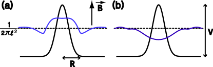
Figure 1: We have plotted schematically electron density for a filled Landau level. The electron density in the absence of the potential is $\frac{1}{2\pi\ell^{2}}$, represented by the dashed horizontal line. In graphene LLs, under certain conditions, induced density can be positive (a), in contrast to the usual case where it is negative (b).

These unusual graphene LLs respond rather differently to presence of potentialsChen ; Sch ; Rec ; Park in comparison with LLs of ordinary semiconductors : Confinement and deconfinement transitions Chen and bound states forming inside an antidot Park through complete Klein tunneling are predicted. Here we consider the electron density in the presence of a rotationally invariant and repulsive potential $V(r)$ with strength $V$ and range $R$. The electron density of the $N$th filled LL is given by

$$n_{N}(r)=\sum_{J\in\textrm{filled Landau level}}|\Psi_{N}^{J}(r)|^{2},$$ (2)

where eigenstates $\Psi_{N}^{J}(r)$ and eigenvalues $E_{N}(J)$ are labeled by LL index $N$ and half-integer angular momentum quantum number $J$. In the absence of a localized potential the dimensionless density takes the value $\ell^{2}n_{N}(r)=\frac{1}{2\pi}$. We define the induced density as the difference between densities with and without the potential

$$\ell^{2}\Delta n_{N}(r)=\ell^{2}n_{N}(r)-\frac{1}{2\pi}.$$ (3)

Graphene barrier has a natural energy scale, $E_{c}=\frac{\hbar v_{F}}{R}$. It is interesting to note that the ratio between this energy scale and the energy scale of LLs is given by the ratio between two length scales of the problem:

$$\frac{E_{m}}{E_{c}}=\frac{R}{\ell}.$$ (4)

We find that the correct scaling function of the induced density has the form

$$\ell^{2}\Delta n_{N}(r)=s_{N}(\frac{r}{R},\frac{V}{E_{c}},\frac{R}{\ell}).$$ (5)

It is different from the scaling function of ordinary LLs where one would expect that $\frac{V}{E_{m}}$ appears instead of $\frac{V}{E_{c}}$. In graphene $\frac{V}{E_{m}}$ does not contain non-perturbative effect of the formation of bound states in the barrier, and it cannot be used instead of $\frac{V}{E_{c}}$. Moreover, the variable $\frac{V}{E_{m}}$ is inappropriate since it becomes infinitely large at zero magnetic field (note $E_{m}=0$ at $B=0$), which leads to the unphysical result that the scaling function is independent of $V$.

The value of the dimensionless electron density at the center of the potential ($r=0$) gives a good indication of how strong the effective coupling constant between the repulsive potential and electrons is. We will thus call this dimensionless induced density at $r=0$, with sign change, as the effective coupling constant

$$\alpha_{N}(\frac{V}{E_{c}},\frac{R}{\ell})=-\ell^{2}\Delta n_{N}(0)=-s_{N}(0,\frac{V}{E_{c}},\frac{R}{\ell}).$$ (6)

As one moves from weak to strong coupling regimes the effective coupling constant becomes increasingly more repulsive, and then starts to decrease, passing through zero, and becomes attractive, see Figs.1 and 2. The strong, intermediate, and weak coupling regimes correspond to $\frac{R}{\ell}\ll 1$, $\frac{R}{\ell}\sim 1$, and $\frac{R}{\ell}\gg 1$, respectively. In the strong coupling regime a repulsive potential can effectively attract electrons, making the induced density positive. The physical origin of this effect is the formation of bound states that are peaked inside the barrier with tails extending over $\ell(N+1)$. We stress that these states are not resonant states of the repulsive potential in graphene at B=0Dong ; Sil ; Matu since the extent of the wavefunctions is finite and their energies form discrete spectra, unlike resonant states.

Figure 2: Y-axis represents values of $g_{0}(R/\ell)$ obtained by data collapse for N=0 and $\frac{V}{E_{c}}<0.7$. Note that this quantity is proportional to $-\alpha_{N}(\frac{V}{E_{c}},\frac{R}{\ell})$. Values $(R/\ell,V/E_{c})$ used in the data collapse are shown in the inset. Note that the induced density changes sign near $R/\ell=1$. Crosses represent the results obtained by treating $V(r)$ in the 2nd order perturbation theory. These results demonstrate that perturbative methods cannot be applied in the intermediate and strong coupling regimes.

In the limit $V/E_{c}\ll 1$ we find the following power laws:

$$\ell^{2}\Delta n_{N}(0)\approx(\frac{V}{E_{c}})^{\delta_{N}}g_{N}(R/\ell)$$ (7)

with $\delta_{N}=2$ for the chiralcom1 $N=0$ LL, but with $\delta_{N}=1$ for non-chiral $N=1$ LL. We find that $g_{0}(R/\ell)$ changes sign near 1. A plot of $g_{0}(R/\ell)$ is shown in Fig.2.

This paper is organized as follows. In Sec.II we present probability wavefunctions of boundstates in weak, intermediate, and strong coupling regimes. Using these probability wavefunctions we investigate scaling properties of induced densities for chiral and non-chiral fermions in Sec.III. We also compute the boundary between positive and negative values of induced densities in the parameter space. Summary and discussions are given in Sec.IV.

II Model calculations of exact wavefunctions

The electron density of a filled LL is computed from single electron wave functions, see Eq.(2). These wave functions are chosen to be eigenstates of the following model potential

$$V(r)=\left\{\begin{array}[]{c}V\ \ \ \ r<R\\ 0\ \ \ \ r>R\end{array}\right..$$ (10)

In the strong coupling regime states with small values of $|J|$ are peaked near $r=0$ and are particularly relevant for the density inside of the potential.

II.1 Energy spectrum

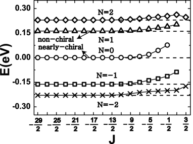
Figure 3: Single particle energy spectrum of massless Dirac fermions in the presence of repulsive potential and magnetic field. Energies of five Landau levels are shown for $N=-2,-1,0,1,2$. Dashed lines represent unperturbed energies, and those that deviate from these are energies of boundstates. (At $B=20$T, $R=10$nm, $R/{\ell}=1.74$, $V=0.1$eV).

Table 1: Eigenstates are labeled by two quantum numbers: LL index $N$ and angular momentum quantum number $J$. Possible values of $N$ and $J$ are listed.

N	J
⋮	⋮
2	$\frac{3}{2}$, $\frac{1}{2}$,$-\frac{1}{2}$,$-\frac{3}{2}$, $-\frac{5}{2}$, $\cdots$
1	$\frac{1}{2}$,$-\frac{1}{2}$,$-\frac{3}{2}$, $-\frac{5}{2}$, $\cdots$
0	$-\frac{1}{2}$,$-\frac{3}{2}$,$-\frac{5}{2}$, $\cdots$
-1	$\frac{1}{2}$,$-\frac{1}{2}$,$-\frac{3}{2}$, $-\frac{5}{2}$, $\cdots$
-2	$\frac{3}{2}$, $\frac{1}{2}$,$-\frac{1}{2}$,$-\frac{3}{2}$, $-\frac{5}{2}$, $\cdots$
⋮	⋮

We compute eigenenergies $E_{N}(J)$ as a function of $J$ by solving Dirac equations. We choose the magnetic vector potential as $\vec{A}=\frac{B}{2}(-y,x,0)$. The two-component wavefunctions of massless Dirac electrons obey the following Hamiltonian

$$H=v_{F}\vec{\sigma}\cdot(\vec{p}+\frac{e}{c}\vec{A})+V(\vec{r})$$ (11)

where the Fermi velocity is $v_{F}$, the Pauli spin matrices are $\vec{\sigma}=(\sigma_{x},\sigma_{y})$. Eigenstates $\Psi_{N}^{J}(\vec{r})$ are also eigenstates of angular momentum operator

$$J_{z}=-i\partial_{\theta}+\frac{\sigma_{z}}{2},$$ (12)

where $\sigma_{z}$ is a Pauli spin matrix and $\theta$ is the polar angle. Since $J_{z}$ commutes with Dirac Hamiltonian of $N$th filled LL eigenstates must have the following form

$$\Psi^{J}_{N}(r,\theta)=e^{i(J-1/2)\theta}\left(\begin{array}[]{c}\chi_{A}(r)\\ \chi_{B}(r)e^{i\theta}\end{array}\right)$$ (15)

with half-integer values of angular quantum number $J$. For each $N$ allowed values of $J$ are displayed in TABLE I. Some eigenenergies are shown in Fig.3. Although this spectrum resembles the spectrum of ordinary LLsYang1 the wavefunctions of the eigenstates are rather different.

II.2 Solutions in strong coupling regime

Table 2: How $\psi_{i}^{J}$ and $\psi_{n,m}$ are related to each other. For a given $J$ some possible values of $(n,m)$ are listed. Empty boxes indicate that $(n,m)$ do not exist.

	$(n_{-3},m_{-3})$	$(n_{-2},m_{-2})$	$(n_{-1},m_{-1})$	$(n_{0},m_{0})$	$(n_{1},m_{1})$	$(n_{2},m_{2})$	$(n_{3},m_{3})$
$\frac{3}{2}$	(-3,1)	(-2,0)				(2,0)	(3,1)
$\frac{1}{2}$	(-3,2)	(-2,1)	(-1,0)		(1,0)	(2,1)	(3,2)
$-\frac{1}{2}$	(-3,3)	(-2,2)	(-1,1)	(0,0)	(1,1)	(2,2)	(3,3)
$-\frac{3}{2}$	(-3,4)	(-2,3)	(-1,2)	(0,1)	(1,2)	(2,3)	(3,4)

It is instructive to study properties of probability wavefunctions in the strong coupling limit, where $R/\ell\rightarrow 0$. Eigenstates $(\chi_{A},\chi_{B})$ are determined by the pair of coupled first order differential equations

$$\left\{\begin{array}[]{c}-i\partial_{x}\chi_{A}+i\Big{[}\frac{1}{x}(J-\frac{1}{2})+\frac{1}{2}x\Big{]}\chi_{A}=\epsilon(x)\chi_{B}\\ -i\partial_{x}\chi_{B}-i\Big{[}\frac{1}{x}(J+\frac{1}{2})+\frac{1}{2}x\Big{]}\chi_{B}=\epsilon(x)\chi_{A}\end{array}\right.,$$ (18)

where $x=r/\ell$ is the dimensionless coordinate and $\epsilon(x)=(E-V(x))/E_{m}$.

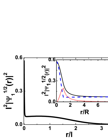
Figure 4: Boundstates of strong coupling limit: $|\Psi_{1}^{1/2}(r)|^{2}$ for $V/E_{c}=1.82$, $R/\ell=0.01$, $R=1$nm, $V=1.2$eV, and $E=0.009$eV. Inset: A (B) component is dashed (dotted) line.

For $r\gg R$ the effect of the potential is negligible, and solutionsToke are

$$\psi_{i}^{J}(\vec{r})=\psi_{n,m}(\vec{r})=C_{n}\left(\begin{array}[]{c}-\textrm{sgn(n)}i\phi_{|n|-1,m}(\vec{r})\\ \phi_{|n|,m}(\vec{r})\end{array}\right).$$ (21)

Here $n$ and $m$ are integers with $m\geq 0$. We define $\textrm{sgn}(n)=-1,0,1$ for $n<0$, $n=0$ and $n>0$. The normalization constant $C_{n}=1$ for $n=0$ and $C_{n}=1/\sqrt{2}$ for $n\neq 0$. Applying angular momentum operator to Eq.(21) and comparing with Eq.(15) we find that the quantum numbers $J$ and $(n,m)$ are related to each other through

$$J=|n|-m-1/2.$$ (22)

For a given value of $J$ there are infinitely many possible values of $(n,m)$, and we will order them with an index $i$. How $(J,i)$ are related to $(n,m)$ is given in Table II. In Eq.(21) the wavefunctions $\phi_{n,m}(\vec{r})$ are the Landau level wavefunctions of ordinary two-dimensional systemsYoshi

$$\phi_{n,m}(\vec{r}) = A_{n,m}\exp\left(i(n-m)\theta-\frac{r^{2}}{4\ell^{2}}\right)\left(\frac{r}{\ell}\right)^{|m-n|}$$ (23)

$$\times L_{(n+m-|m-n|)/2}^{|m-n|}\left(\frac{r^{2}}{2\ell^{2}}\right),$$

where $A_{n,m}$ are normalization constants.

To find solutions that are valid for all $r$, we solve the Dirac equations numerically using confluent hypergeometric functionsRec . The obtained numerical results are shown of Fig.4. Near $x\geq R/\ell$ the value of the eigenfunction $\psi_{N}^{J}(r)$ is approximately equal to $\psi_{i}^{J}(R)$, given by Eq.(21). Both A- and B-components of the eigenfunction vary rapidly for $r\leq R$. For $J=1/2$ the A-component of the wavefunction $\chi_{A}(x)$ is peaked at $x=0$ while B-component is peaked at $x=R/\ell$. These peak values of both $\chi_{A}$ and $\chi_{B}$ approach finite values in the limit $R/\ell\rightarrow 0$. However, as $V/E_{c}$ increases they also increase. The amount of jump between $0$ and $R$ is, consistent with Eq.(18),

$$-i\Delta\chi_{A}=-i(\chi_{A}(R)-\chi_{A}(0))\approx\epsilon(0)\int_{0}^{R/\ell}dx\chi_{B}$$ (24)

with $\chi_{B}(0)=0$ and $\epsilon(0)=(E-V)/E_{m}$. For $J=-1/2$ the properties are the opposite to those of $J=1/2$: the B-component of the wavefunction $\chi_{B}(x)$ peaked at $x=0$ while A-component is peaked at $x=R/\ell$. The amount of jump between $0$ and $R$ is

$$-i\Delta\chi_{B}\approx\epsilon(0)\int_{0}^{R/\ell}dx\chi_{A}.$$ (25)

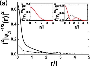
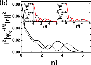
Figure 5: Strong coupling regime: the parameters are $E_{c}=0.1316$ eV, $E_{m}=0.0395$ eV, $V=0.26$eV, $V/E_{c}=1.98$ and $R/\ell=0.3$. (a) Solid line is for $N=0$ and $E=0.017$ eV. Dashed line is for $N=1$ and $E=0.061$ eV. Inset: B-component of $|\Psi_{0}^{-1/2}(r)|^{2}$ and A- (dashed) and B- (solid) components of $|\Psi_{1}^{-1/2}(r)|^{2}$ in the absence of potential. (b) Solid line is for $N$=2 and $E=0.083$ eV. Dashed line is for $N=3$ and $E=0.101$ eV. Inset: A- and B-components of $|\Psi_{2}^{-1/2}(r)|^{2}$ and $|\Psi_{3}^{-1/2}(r)|^{2}$ in the absence of potential.

In the strong coupling regime $R/\ell<1$ probability wavefunctions can be significant inside the potential, see Fig.5. These states are peaked inside the potential range $R$ and have tails extending over the length of order $\ell(N+1)$. Examples of such states with $N=0,1,2,$ and $3$ are displayed in Fig.5. As $N$ increases the extend of $|\Psi_{N}^{-1/2}(r)|^{2}$ outside the potential increases approximately as $\ell(N+1)$. However, the strength of peak within the range $R$ decreases with increasing $N$. We stress that these states are not resonant states of the repulsive potential since the extend of the wavefunctions is finite and their energies form discrete spectra, unlike resonant states. States shown in Fig.5 contribute to a positive induced charge since the probability of finding an electron inside the potential has increased compared to the probability in the absence of the potential. This is a non-trivial effect of the interplay between effects of quantization of LL and Klein tunnelingKat ; Sta .

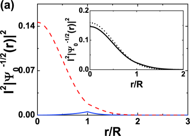
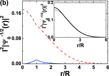
Figure 6: (a) Weak coupling regime: $|\Psi_{0}^{-1/2}(r)|^{2}$ for $R/\ell=2.0$, $V/E_{c}=2.172$, $R=11$nm, $V=0.13$eV, and $E=0.110$eV. A (B) component is solid (dashed) line. Inset: dashed line is without potential and solid is with potential. (b) Intermediate coupling regime: $|\Psi_{0}^{-1/2}(r)|^{2}$ for $R/\ell=0.6$, $V/E_{c}=0.607$, $R=5$nm, $V=0.08$eV, and $E=0.013$eV.

II.3 Solutions in intermediate and weak coupling regimes

We show how probability wavefunctions change as $R/\ell$ changes from weak to intermediate coupling regimes. In the perturbative regime $R/\ell\gg 1$ the exact probability wavefunction at $r=0$ is smaller than that of the unperturbed probability wavefunction, as shown in Fig.6(a). Note that cusps in the wavefunctions are negligible. Fig.6(b) displays the exact probability wavefunctions $|\Psi_{0}^{-1/2}(r)|^{2}$ in the intermediate regime of $R/\ell\sim 1$. Both A and B components of it have cusps at $r=R$. Note that at $r=0$ the exact probability wavefunction is larger than that of the unperturbed probability wavefunction.

III scaling function of electron density

Figure 7: (a) $\ell^{2}n(r)$ for $N=0$ and $R/\ell\leq 1$. $(\frac{R}{\ell},\frac{V}{E_{c}})=(1,1.215)$ (solid), $(\frac{R}{\ell},\frac{V}{E_{c}})=(0.60,0.607)$ (dashed), $(\frac{R}{\ell},\frac{V}{E_{c}})=(0.30,0.334)$ (dot). Dashed-dot line is $\ell^{2}n(r)$ in the absence of the potential. (b) For $N=0$ and $R/\ell>1$. $(\frac{R}{\ell},\frac{V}{E_{c}})=(1.74,2.582)$ (solid), $(\frac{R}{\ell},\frac{V}{E_{c}})=(1.50,1.823)$ (dashed), $(\frac{R}{\ell},\frac{V}{E_{c}})=(1.22,1.063)$ (dot).

Figure 8: Approximate data collapse of $g_{0}(R/\ell)$ is obtained for a larger range of $\frac{V}{E_{c}}$ than the one used in Fig.2 . Values of $(\frac{V}{E_{c}},R/\ell)$ used are shown in inset.

We have performed an extensive numerical evaluation of the electron density. The dimensionless induced density for $N=0$ filled LL, $\ell^{2}\Delta n_{0}(r/R)$, is plotted in Fig.7 for various values of $(R/\ell,\frac{V}{E_{c}})$. For $R/\ell<1$ the induced density inside the barrier is positive, which is in sharp contrast to what usually happens in a barrier. The formation of bound states inside the barrier, as discussed in Sec. II B, is responsible for this effect. Note the induced density oscillates as a function of $r/R$. We have tested that the total integrated density is equal to the total number of electrons in the LL. The induced density satisfies the following two-parameter scaling function

$$\ell^{2}\Delta n_{0}(r/R)=s_{0}(r/R,\frac{V}{E_{c}},R/\ell).$$ (26)

As $R/\ell$ increases the sign of $\Delta n_{0}(0)$ changes sign from plus to minus, which is shown in Fig.7. Physically this means positive induced density changes to negative induced density. For $\frac{V}{E_{c}}<0.7$ our numerical results display data collapse, and is consistent with the following power law

$$\ell^{2}\Delta n_{0}(0)\approx(\frac{V}{E_{c}})^{2}g_{0}(R/\ell),$$ (27)

see Fig.2. For a larger range of $\frac{V}{E_{c}}<2.5$ an approximate data collapse can be obtained, see Fig.8.

The second order perturbative calculation in $V(r)$ agrees with scaling result when $R/\ell>2.5$, but disagrees when $R/\ell<2$, as shown in Fig.2. It is noteworthy that $g_{0}(R/\ell)$ takes the minimum value near $R/\ell\approx 1.5$. This implies that the electron density is depleted most strongly for $R/\ell\approx 1.5$. However, further decrease in $R/\ell$ has the opposite effect of increasing more penetration of electrons into the barrier. Near $R/\ell=1$ the scaling function $g_{0}(R/\ell)$ changes sign. For $R/\ell<1$ electrons accumulate in the barrier and the density becomes greater than the density of the unperturbed LL. This dependence on $R/\ell$ is thus strongly non-linear. For larger values of $V/E_{c}$ the boundary between positive and negative induced densities is displayed in Fig.9.

Figure 9: $N=0$ LL states must not overlap with $N=\pm$ 1 LLs. Induced density at $r=0$ is positive for $R/\ell<1$.

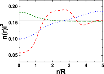
Figure 10: $\ell^{2}n(r)$ for $N=1$. $(\frac{R}{\ell},\frac{V}{E_{c}})=(1.5,3.038)$ (dashed), $(\frac{R}{\ell},\frac{V}{E_{c}})=(0.6,0.607)$ (dot), $(\frac{R}{\ell},\frac{V}{E_{c}})=(0.01,0.607)$ (dashed dot). Solid line is $\ell^{2}n(r)$ in the absence of the potential.

Figure 11: $g_{1}(R/\ell)$ is obtained by data collapse for $N=1$ and $\frac{V}{E_{c}}\ll 1$ . Values of $(\frac{V}{E_{c}},R/\ell)$ used are shown in inset.

The induced density for $N=1$ filled LL shown in Fig.10 satisfies a similar scaling relation as that of $N=0$ LL

$$\ell^{2}\Delta n_{1}(r/R)=s_{1}(r/R,\frac{V}{E_{c}},R/\ell).$$ (28)

At the origin $r=0$ we find, for $\frac{V}{E_{c}}\ll 1$, the following scaling result

$$\ell^{2}\Delta n_{1}(0)\approx(\frac{V}{E_{c}})^{\delta_{1}}g_{1}(R/\ell),$$ (29)

where $\delta_{1}=1$. This result is obtained in the range $V/E_{c}<0.1$ by data collapsing numerical data points, see Fig.11. The dependence of the induced density on $R/\ell$ is again strongly non-linear: $g_{1}(R/\ell)$ takes the minimum value near $R/\ell=0.7$. For larger values of $\frac{V}{E_{c}}$ the boundary between positive and negative induced densities is displayed in Fig.12. As $\frac{V}{E_{c}}$ increases the range of $R/\ell$ where the induced density is positive expands. Note that for small values of $R/\ell$, for example 0.01, the value of $\ell$ at B=1T is $257\AA$ and R becomes comparable to the lattice constant so that Dirac equations breakdown. In this case smaller values of B must be used so that R can take larger values.

It can shown from perturbative analysis that, for chiral fermions, the first order correction of $V(r)$ absent, but the second order correction is present and is negative. The absence of the linear terms in $\frac{V}{E_{c}}$ for the chiral $N=0$ LL is a consequence of the symmetric properties of conduction and valence band LLs. However, for non-chiral fermions the first order correction is present. These results are consistent with non-perturbative scaling results given by Eqs.(27) and (29).

Figure 12: $N=1$ LL states must not overlap with $N=0,2$ LLs. The range of $R/\ell$, where the induced density at $r=0$ is positive increases with increasing $V/E_{c}$.

We now mention some general properties of the induced density of LLs. It has a critical point $y_{c,1}$, where

$$\frac{\partial s_{N}(0,x,y)}{\partial y}\Big{|}_{y=y_{c,1}}=0$$ (30)

($x=\frac{V}{E_{c}}$ and $y=\frac{R}{\ell}$). We find that $y_{c,1}\sim 1$. The scaling function takes the global minimum at $y_{c,1}$: as $y$ decreases the induced density becomes most negative at $y=y_{c,1}$ and then it increases, in contrast to the lowest order perturbative result in $V$, which suggests that it becomes increasingly more negative as $y$ decreases. Below this critical point perturbative methods are inapplicable, and it separates strong and weak coupling regimes. The sign of the induced density changes at the second critical point $y_{c,2}$, where

$$s_{N}(0,x,y)|_{y=y_{c,2}}=0.$$ (31)

As $y$ decreases below $y=y_{c,1}$ the induced density changes sign at $y=y_{c,2}$ and begins to take positive values.

IV summary and discussions

We find that a repulsive potential of graphene has bound states that are peaked inside the barrier with tails extending over $\ell(N+1)$. The properties of these boundstates change as $R/\ell$ varies, and affect the induced density of filled LLs inside the barrier in a non-trivial way as a function of $R/\ell$. As $R/\ell$ decreases the induced density inside the barrier becomes more negative, but as it reaches a critical value the induced density reaches an extremum value. Upon further decrease of $R/\ell$ the value of the induced density reaches zero, and, after this, it becomes positive. These changes are strongly non-linear in $R/\ell$, and one moves successively from weak, intermediate, and strong coupling regimes as $R/\ell$ decreases. The condition $V/E_{c}\ll 1$ is not sufficient for treating $V(r)$ perturbatively, and, in addition to this, one must require $R/\ell\gg 1$ for both chiral and non-chiral fermions.

For filled LLs electron-electron interactions may be approximated well by a Hartree-Fock (HF) methodMac . The electron density in HF method is given by the sum of unrenormalized single electron probability wavefunctions, just as in Eq.(2). So our calculation of the induced density is actually a HF result. However, our single electron energies are not the renormalized HF result. This will somewhat affect our numerical estimate of the boundary between overlapping LLs of Figs.9 and 12. The discontinuity in the potential of Eq.(10) can couple states in K and K^′ valleys, which is ignored in our approach. However, our tight-binding calculations show that this coupling is smallPark .

There is a symmetryPark between repulsive and attractive potentials $V(r)$ and $-V(r)$ so that the induced densities of these potentials are identical. In the presence of a repulsive or attractive potential, both charge accumulation and depletion occur, depending on the value of $R/\ell$, see Figs.9 and 12. The appearance of a charge accumulation near a repulsive potential, for example, could be explained by introducing an attractive potential via the transformation $V(r)\rightarrow-V(r)$, but this same transformation would fail to explain charge depletion since electrons would pile up around the transformed attractive potential. Thus charge depletion and accumulation cannot be explained simultaneously in either perspective of repulsive or attractive potential. In addition, the critical points $R/\ell=y_{c,1}$ and $y_{c,2}$, where the scaling function takes the global minimum and where it changes sign cannot be explained by application $V(r)\rightarrow-V(r)$. It would be desirable to construct an analytic theory for them.

Properties of the bound states of the potential barrier may be observed as follows. A localized potential may be created by a circular gate placed on graphene sheet. When this gate is sufficiently close to the edge of the sample coupling between bound states and edge states may be induced, and the transmission coefficients of edge states may reveal properties of the bound states. Also these boundstates may play an important role in transport and magnetic properties of grapheneHuang .

S.R.E.Y. thanks Philip Kim for valuable discussions on various aspects of this paper. This work was supported by the Korea Research Foundation Grant funded by the Korean Government (KRF-2009-0074470).

References

- (1) K. S. Novoselov, A. K. Geim, S. V. Morozov, D. Jiang, Y. Zhang, S. V. Dubonos, I. V. Grigorieva, A. A. Firsov, Science, 306, 666 (2004).
- (2) A. K. Geim and A. H. MacDonald, Phys. Today, 60(8), 35 (2007).
- (3) T. Ando, J. Phys. Soc. Jpn. 74, 777 (2005).
- (4) A. H. Castro Neto, F. Guinea, N. M. R. Peres, K. S. Novoselov, and A. K. Geim, Rev. Mod. Phys. 81, 109 (2009).
- (5) V. P. Gusynin, and S. G. Sharapov, Phys. Rev. Lett. 95, 146801 (2005).
- (6) Y. Zhang, Y. W. Tan, H. L. Stormer, P. Kim, Nature, 438, 201 (2005).
- (7) D. L. Miller, K. D. Kubista, G. M. Rutter, M. Ruan, W. A. de Heer, P. N. First, and J. A. Stroscio, Science, 324, 924 (2009).
- (8) K. I. Bolotin, F. Ghahari, M. D. Shulman, H. L. Stormer, and P. Kim, Nature, 462, 196 (2009).
- (9) Y. Zheng and T. Ando, Phys. Rev. B 65, 245420 (2002).
- (10) C. Tőke, P. E. Lammert, V. H. Crespi, and J. K. Jain, Phys. Rev. B 74, 235417 (2006).
- (11) M. L. Sadowski, G. Martinez, M. Potemski, C. Berger, and W. A. de Heer, Phys. Rev. Lett. 97, 266405 (2006).
- (12) R. S. Deacon, K. -C. Chuang, R. J. Nicholas, K. S. Novoselov, and A. K. Geim, Phys. Rev. B 76, 081406R (2007).
- (13) H. Y. Chen, V. Apalkov, and T. Chakraborty, Phys. Rev. Lett. 98, 186803 (2007); G. Giavaras, P.A. Maksim, and M. Roy, J. Phys.: Condens. Matter 21, 102201 (2009).
- (14) S. Schnez, K. Ensslin, M. Sigrist, and T. Ihn, Phys. Rev. B 78, 195427 (2008).
- (15) P. Recher, J. Nilsson, G. Burkard, B. Trauzettel, Phys. Rev. B 79, 085407 (2009).
- (16) P. S. Park, S. C. Kim, and S.-R. Eric Yang, J. Phys.: Condens. Matter 22, 375302 (2010).
- (17) S.-H. Dong, X.-W. Hou, and Z.-Q. Ma, Phys. Rev. A 58, 2160, (1998).
- (18) P. G. Silvestrov and K. B. Efetov, Phys. Rev. Lett. 98, 016802, (2007).
- (19) A. Matulis and F. M. Peeters, Phys. Rev. B 77, 115423 (2008).
- (20) It should be noted that a localized potential couples chiral LL states to non-chiral LL states, and thus makes the band states slightly non-chiral. Since these states are dominantly chiral we will call them chiral states. In states both A and B components are present, and these states are non-chiral.
- (21) S. -R. Eric Yang and A. H. MacDonald, Phys. Rev. B, 42, 10811R (1990).
- (22) D. Yoshioka, The Quantum Hall Effect (Springer, Berlin, 1998).
- (23) M. I. Katsnelson, K. S. Novoselov, and A. K. Geim, Nature Phys. 2, 620 (2006).
- (24) N. Stander, B. Huard, and D. Goldhaber-Gordon, Phys. Rev. Lett. 102, 026807 (2009).
- (25) A. H. MacDonald, S. -R. Eric Yang, and M. D. Johnson, Aust. J. Phys. 46, 345 (1993); S. -R. Eric Yang, A. H. MacDonald, and M. D. Johnson, Phys. Rev. Lett. 71, 3194 (1993).
- (26) B.-L. Huang, M.-C. Chang, and C.-Y. Mou, Phys. Rev. B, 82, 155462 (2010); H. Ohldag, T. Tyliszczak, R. Hohne, D. Spemann, P. Esquinazi, M. Ungureanu, and T. Butz, Phys. Rev. Lett. 98, 187204 (2007).