Phase transitions in the three-state Ising spin-glass model with finite connectivity

Abstract

The statistical mechanics of a two-state Ising spin-glass model with finite random connectivity, in which each site is connected to a finite number of other sites, is extended in this work within the replica technique to study the phase transitions in the three-state Ghatak-Sherrington (or random Blume-Capel) model of a spin glass with a crystal field term. The replica symmetry ansatz for the order function is expressed in terms of a two-dimensional effective-field distribution which is determined numerically by means of a population dynamics procedure. Phase diagrams are obtained exhibiting phase boundaries which have a reentrance with both a continuous and a genuine first-order transition with a discontinuity in the entropy. This may be seen as “inverse freezing”, which has been studied extensively lately, as a process either with or without exchange of latent heat.

Introduction

Numerous problems of frustrated, disordered systems, with extensive connectivity in which each site is linked to a macroscopic number of other sites Ni01 have been studied in the past by means of the replica technique in mean-field theory SK76 ; PMV87 . The technique has been extended to systems with finite random connectivity and binary units (spins) in states $\sigma=\pm 1$, in which each site is linked to a finite number of other sites, in areas like error correcting codes MK00 ; NK01 ; Ni01 , spin glasses VB85 ; KS87 ; MP87 ; WS88 ; Mo98 ; MP01 , neural networks WC03 ; PS03 ; PW04 and small-world lattices NC04 . The fact that mean-field theory is exact only for infinite-range interactions or infinite-dimensional systems has been a challenge for the understanding of the behavior of more realistic disordered systems, and a study of the effects of finite connectivity even in mean-field theory could be a useful improvement.

Three-state spin models of states $\sigma=0,\pm 1$ with random bonds and finite connectivity could be of interest to condensed matter physics in view of the phase transitions that already appear, within mean-field theory, in the random Blume-Emery-Griffith-Capel (BEGC) model with full connectivity between the spins CL04 ; CL05 and it should also be of interest for information processing in neural networks Bo04 . The simplest case of a fully connected random BEGC model is the three-state spin-glass model of Ghatak and Sherrington (GS) GS77 ; CYS94 , which is a Blume-Capel (BC) model with random bonds BC66 . The GS model with infinite range interactions exhibits both a continuous transition at high $T$ and a genuine thermodynamic first-order transition below a tricritical point between a spin-glass and a paramagnetic phase. The first-order transition appears in a reentrant part of the phase boundary and it may describe "inverse freezing" with an exchange of latent heat. This is a reversible transition, say between a paramagnetic (P) phase and a spin-glass (SG) phase in which the entropy of the P phase below the transition is smaller than the entropy of the SG phase and there has been a recent revival of interest in these transitions SS03 ; PL10 which could explain the behavior of colloidal and polymeric systems, among others (see ref. PL10 for a recent summary of realizations).

A result of the GS model, either in mean-field theory with full connectivity or obtained by means of numerical simulations for nearest-neighbor interactions in three dimensions, is that the tricritical point separating the continuous and the first-order transition is either above or at the point of reentrance on the phase boundary implying that inverse freezing appears only as a first-order transition CL04 ; CL05 ; PL10 .

General results in the form of complete phase diagrams of stationary states for the GS (or random BC) model with finite connectivity are still missing and the purpose of this paper is to make progress in that direction by means of an analytic study extending the SG replica technique, with the replica-symmetry (RS) ansatz, developed for disordered Ising systems with finite random connectivity and binary spins NC04 . Typical questions one would like to answer is how the nature of the transition changes with the connectivity, if there is reentrance behavior of the phase boundaries and if this takes place either as a continuous or as a first-order transition at finite temperature.

The procedure on which the present work is based introduces an order-function KS87 , in place of an infinite number of order parameters VB85 , and uses a representation in terms of a weighted probability of alignment of the spins involving a distribution of a two-component local field. One of the components is associated to a linear form in the spins, while the other component is associated to the crystal field term. A population dynamics technique is used to solve numerically a self-consistency equation for the distribution of the local field that yields the relevant physical order parameters. Phase diagrams are then obtained which exhibit either a continuous transition between a P and a SG phase, for low connectivity, or both a continuous and a first-order phase transition that merge at a tricritical point with reentrance behavior characteristic of inverse freezing between those phases, for increasing finite connectivity.

The outline of the paper is the following. In section 2 we present the GS model and carry out the replica procedure that yields the statistical mechanics for the three-state system. In section 3 we present the results for the distribution of local fields, the relevant order parameters and the free energy and discuss the phase diagrams. We conclude in section 4 with a summary and remarks.

The model and replica procedure

We consider a system of $N$ interacting three-state Ising spins $\sigma_{i}\in\{-1,0,1\}$, $i=1\dots N$, described by the Hamiltonian

$$H=-\frac{1}{c}\sum_{i<j}c_{ij}J_{ij}\sigma_{i}\sigma_{j}+D\sum_{i}\sigma_{i}^{2}\,.$$ (1)

The random variable $c_{ij}\in\{0,1\}$ indicates whether there is a connection $(c_{ij}=1)$ or not $(c_{ij}=0)$ between a pair of spins $(i,j)$ and it takes different values for different pairs of spins, according to the distribution

$$p\left(c_{ij}\right)=\frac{c}{N}\delta_{c_{ij},1}+\left(1-\frac{c}{N}\right)\delta_{c_{ij},0}\,\,\,,$$ (2)

where $c$ (the connectivity) is the average number of connections per spin which is assumed to remain finite in the thermodynamic limit $N\rightarrow\infty$, such that $c/N\rightarrow 0$. Thus, the sites are connected according to a Poisson distribution, and one makes use of this limit in deriving the statistical mechanics of the system. There is a set of infinite-range interactions $\{J_{ij}\}$ that will be assumed to be independent, identically distributed, random variables drawn from a distribution $p(J_{ij})$, to be specified below, and averages over that distribution of a quantity $g(J_{ij})$ will be denoted by ${\langle g(J)\rangle}_{J}$. The quadratic form in the spins favors the population of the zero state, if $D>0$, or the states $\pm 1$, if $D<0$. If $D$ is sufficiently large and negative one retrieves the binary Ising spin-glass model with finite connectivity and spins $\sigma_{i}\in\{-1,1\}$, which is a particular case of the recently studied small world spin glasses when the nearest neighbor interaction along the ring is set to zero NC04 .

Assuming thermal equilibrium at an inverse temperature $\beta=1/T$, the disorder-averaged free energy per spin is calculated in the replica procedure as

$$f(\beta)=-\lim_{N\rightarrow\infty}\frac{1}{\beta N}\lim_{n\rightarrow 0}\frac{1}{n}\log\langle{Z^{n}}\rangle\,\,\,,$$ (3)

where

$$Z=\sum_{\sigma_{1}\dots\sigma_{N}}{\mathrm{e}}^{-\beta H}$$ (4)

is the partition function and the brackets stand for the disorder average. In the small $c/N$ limit, the disorder-average replicated partition function becomes, to leading order in $N$,

$$\left\langle Z^{n}\right\rangle=\sum_{\mbox{\boldmath$\sigma$}^{1}\cdots\mbox{\boldmath$\sigma$}^{n}}\exp\left[-\beta D\sum_{i,\alpha}\left(\sigma_{i}^{\alpha}\right)^{2}+\frac{c}{2N}\sum_{i\neq j}\left\langle{\mathrm{e}}^{\frac{1}{c}\beta J\sum_{\alpha}\sigma_{i}^{\alpha}\sigma_{j}^{\alpha}}-1\right\rangle_{J}\right]\,\,\,$$ (5)

where $\alpha=1,\dots,n$ denotes the replica index. Since the connectivity $c$ is finite, one cannot expand the inner exponential and follow the standard infinite-connectivity calculation. Instead, to extract the variables under summation from the inner exponential, one introduces the identity

$$1=\sum_{\mbox{\boldmath$\sigma$}}\delta_{\mbox{\boldmath$\sigma$}\mbox{\boldmath$\sigma$}_{i}}\equiv\sum_{\mbox{\boldmath$\sigma$}}\prod_{\alpha=1}^{n}\delta_{\sigma^{\alpha}\sigma_{i}^{\alpha}}\,,$$ (6)

where $\sigma$ and $\mbox{\boldmath$\sigma$}_{i}$ are $n$-component vectors representing replica states and $\delta_{\mbox{\boldmath$\sigma$}\mbox{\boldmath$\sigma$}_{i}}=1$ if $\mbox{\boldmath$\sigma$}=\mbox{\boldmath$\sigma$}_{i}$ and zero otherwise. Thus, we write

$$\left\langle Z^{n}\right\rangle=\sum_{\mbox{\boldmath$\sigma$}^{1}\cdots\mbox{\boldmath$\sigma$}^{n}}\exp\left[-\beta D\sum_{i,\alpha}\left(\sigma_{i}^{\alpha}\right)^{2}+\frac{c}{2N}\sum_{i\neq j}\sum_{\mbox{\boldmath$\sigma$}\mbox{\boldmath$\tau$}}\delta_{\mbox{\boldmath$\sigma$}\mbox{\boldmath$\sigma$}_{i}}\delta_{\mbox{\boldmath$\tau$}\mbox{\boldmath$\sigma$}_{j}}\left\langle{\mathrm{e}}^{\frac{1}{c}\beta J\sum_{\alpha}\sigma^{\alpha}\tau^{\alpha}}-1\right\rangle_{J}\right]$$ (7)

and introduce the order function $P(\mbox{\boldmath$\sigma$})=(1/N)\sum_{i}\delta_{\mbox{\boldmath$\sigma$}\mbox{\boldmath$\sigma$}_{i}}$, which represents the fraction of sites with the replica configuration $\sigma$, through the identity

$$1=\int\prod_{\mbox{\boldmath$\sigma$}}dP(\mbox{\boldmath$\sigma$})d\hat{P}(\mbox{\boldmath$\sigma$}){\mathrm{e}}^{\sum_{\mbox{\boldmath$\sigma$}}\hat{P}(\mbox{\boldmath$\sigma$})\left(P(\mbox{\boldmath$\sigma$})-\frac{1}{N}\sum_{i}\delta_{\mbox{\boldmath$\sigma$}\mbox{\boldmath$\sigma$}_{i}}\right)}\,\,\,,$$ (8)

where $\hat{P}$ is an auxiliary density. Performing the trace and changing $\hat{P}$ to $N\hat{P}$ the integral

$$\left\langle Z^{n}\right\rangle=\int\prod_{\mbox{\boldmath$\sigma$}}dP(\mbox{\boldmath$\sigma$})d\hat{P}(\mbox{\boldmath$\sigma$})\exp N \left[\sum_{\mbox{\boldmath$\sigma$}}\hat{P}(\mbox{\boldmath$\sigma$})P(\mbox{\boldmath$\sigma$})+\log\sum_{\mbox{\boldmath$\sigma$}}{\mathrm{e}}^{-\beta D\sum_{\alpha}\sigma_{\alpha}^{2}-\hat{P}(\mbox{\boldmath$\sigma$})}\right.$$

$$\quad\quad\quad\left.+\frac{c}{2}\sum_{\mbox{\boldmath$\sigma$}\mbox{\boldmath$\tau$}}P(\mbox{\boldmath$\sigma$})P(\mbox{\boldmath$\tau$})\left\langle{\mathrm{e}}^{\frac{1}{c}\beta J\sum_{\alpha}\sigma_{\alpha}\tau_{\alpha}}-1\right\rangle_{J}\right]\,$$ (9)

can be evaluated by the saddle-point method in the large-$N$ limit, leading to the extremum

$$f(\beta)=-\lim_{n\rightarrow 0}\frac{1}{\beta n}\rm Extr \left[\sum_{\mbox{\boldmath$\sigma$}}\hat{P}(\mbox{\boldmath$\sigma$})P(\mbox{\boldmath$\sigma$})+\log\sum_{\mbox{\boldmath$\sigma$}}{\mathrm{e}}^{-\beta D\sum_{\alpha}\sigma_{\alpha}^{2}-\hat{P}(\mbox{\boldmath$\sigma$})}\right.$$

$$\quad\quad\quad\quad\quad\quad\left.+\frac{c}{2}\sum_{\mbox{\boldmath$\sigma$}\mbox{\boldmath$\tau$}}P(\mbox{\boldmath$\sigma$})P(\mbox{\boldmath$\tau$})\left\langle{\mathrm{e}}^{\frac{1}{c}\beta J\sum_{\alpha}\sigma_{\alpha}\tau_{\alpha}}-1\right\rangle_{J}\right]\,$$ (10)

over the densities $\{P(\mbox{\boldmath$\sigma$}),\hat{P}(\mbox{\boldmath$\sigma$})\}$ for the free energy per site. The saddle-point equations become

$$P(\mbox{\boldmath$\sigma$})=\dfrac{{\mathrm{e}}^{-\beta D\sum_{\alpha}\sigma_{\alpha}^{2}-\hat{P}(\mbox{\boldmath$\sigma$})}}{\sum_{\mbox{\boldmath$\sigma$}}{\mathrm{e}}^{-\beta D\sum_{\alpha}\sigma_{\alpha}^{2}-\hat{P}(\mbox{\boldmath$\sigma$})}}$$ (11)

and

$$\hat{P}(\mbox{\boldmath$\sigma$})=-c\sum_{\mbox{\boldmath$\tau$}}P(\mbox{\boldmath$\tau$})\left\langle{\mathrm{e}}^{\frac{1}{c}\beta J\sum_{\alpha}\sigma_{\alpha}\tau_{\alpha}}-1\right\rangle_{J}\,.$$ (12)

Eliminating $\hat{P}(\mbox{\boldmath$\sigma$})$ in Eq. (11) by means of this expression we obtain the self-consistency relationship

$$P(\mbox{\boldmath$\sigma$})=\dfrac{\exp\left(-\beta D\sum_{\alpha}\sigma_{\alpha}^{2}+c\sum_{\mbox{\boldmath$\tau$}}P(\mbox{\boldmath$\tau$})\left\langle{\mathrm{e}}^{\frac{1}{c}\beta J\sum_{\alpha}\sigma_{\alpha}\tau_{\alpha}}-1\right\rangle_{J}\right)}{\sum_{\mbox{\boldmath$\sigma$}}\exp\left(-\beta D\sum_{\alpha}\sigma_{\alpha}^{2}+c\sum_{\mbox{\boldmath$\tau$}}P(\mbox{\boldmath$\tau$})\left\langle{\mathrm{e}}^{\frac{1}{c}\beta J\sum_{\alpha}\sigma_{\alpha}\tau_{\alpha}}-1\right\rangle_{J}\right)}\,$$ (13)

and the free energy becomes

$$f(\beta)=-\lim_{n\rightarrow 0} \frac{1}{\beta n}\left[-\frac{c}{2}\sum_{\mbox{\boldmath$\sigma$}\mbox{\boldmath$\tau$}}P(\mbox{\boldmath$\sigma$})P(\mbox{\boldmath$\tau$})\left\langle{\mathrm{e}}^{\frac{1}{c}\beta J\sum_{\alpha}\sigma_{\alpha}\tau_{\alpha}}-1\right\rangle_{J}\right.$$ (14)

$$\left.+\log\sum_{\mbox{\boldmath$\sigma$}}\exp\left(-\beta D\sum_{\alpha}\sigma_{\alpha}^{2}+c\sum_{\mbox{\boldmath$\tau$}}P(\mbox{\boldmath$\tau$})\left\langle{\mathrm{e}}^{\frac{1}{c}\beta J\sum_{\alpha}\sigma_{\alpha}\tau_{\alpha}}-1\right\rangle_{J}\right)\right]^{*}\,.$$

with the order function given by the saddle-point equation, indicated by the asterisk.

Our search for solutions of Eq.(13) will be restricted to the replica symmetry (RS) ansatz, KS87 ; Mo98 . This means that $P(\mbox{\boldmath$\sigma$})$ should remain invariant under replica permutations and, consequently, for three-state spins it should only depend on the summations $\sum_{\alpha}\sigma_{\alpha}$ and $\sum_{\alpha}\left(\sigma_{\alpha}\right)^{2}$, with their corresponding weights. Thus, in extension of the RS ansatz for the order function in finite-connectivity two-state Ising models NC04 , we assume that for the three-state model

$$P(\mbox{\boldmath$\sigma$})=\int dh\,db\,W(h,b)\dfrac{{\mathrm{e}}^{\beta h\sum_{\alpha}\sigma_{\alpha}-\beta b\sum_{\alpha}\sigma_{\alpha}^{2}}}{\left[2{\mathrm{e}}^{-\beta b}\cosh(\beta h)+1\right]^{n}}\,\,\,,$$ (15)

for any real $n$, where $h$ and $b$ are the two components of the local field and $W(h,b)$ is a density which has to be determined self-consistently. Since the normalization factors, both here and in Eq.(13), become one in the limit $n\rightarrow 0$ we may leave them aside. Expanding the second exponential in Eq.(13) and using the RS ansatz we have

$$P(\mbox{\boldmath$\sigma$})={\mathrm{e}}^{-\beta D\sum_{\alpha}\sigma_{\alpha}^{2}}\sum_{k=0}^{\infty}\frac{{\mathrm{e}}^{-c}c^{k}}{k!} \int\prod_{l=1}^{k}dh_{l}\,db_{l}\,W\left(h_{l},b_{l}\right)dJ_{l}\,p\left(J_{l}\right)$$

$$\prod_{l=1}^{k}\exp\left[\sum_{\alpha}\log\sum_{\tau_{\alpha}^{l}}{\mathrm{e}}^{\beta h_{l}\tau_{\alpha}^{l}-\beta b_{l}\left(\tau_{\alpha}^{l}\right)^{2}+\frac{1}{c}\beta J_{l}\sigma_{\alpha}\tau_{\alpha}^{l}}\right]\,\,,$$ (16)

where $p\left(J\right)$ is the probability distribution for the interaction, assumed to be continuous. Summing over $\tau_{\alpha}^{l}$ and using the identity $\sum_{\sigma}\delta_{\sigma\sigma_{\alpha}}=1$, in order to extract the appropriate dependence on $\sum_{\alpha}\sigma_{\alpha}$ and $\sum_{\alpha}\left(\sigma_{\alpha}\right)^{2}$, we obtain

$$P(\mbox{\boldmath$\sigma$})={\mathrm{e}}^{-\beta D\sum_{\alpha}\sigma_{\alpha}^{2}} \sum_{k=0}^{\infty}\frac{{\mathrm{e}}^{-c}c^{k}}{k!}\int\prod_{l=1}^{k}dh_{l}\,db_{l}\,W\left(h_{l},b_{l}\right)dJ_{l}\,p\left(J_{l}\right)$$

$$\prod_{l=1}^{k}\exp\sum_{\alpha}\sum_{\sigma}\delta_{\sigma\sigma_{\alpha}}\log\left[2\cosh\left(\beta h_{l}+\beta J_{l}\sigma/c\right){\mathrm{e}}^{-\beta b_{l}}+1\right]\,.$$ (17)

For three-state spins we use the representation

$$\delta_{\sigma\sigma_{\alpha}}=1-\sigma^{2}-\sigma_{\alpha}^{2}+\sigma\sigma_{\alpha}/2+3\sigma^{2}\sigma_{\alpha}^{2}/2\,$$ (18)

to do the sum over $\sigma$ and with the RS ansatz in the left hand side of the equation we obtain the self-consistency relationship for $W(h,b)$,

$$W(h,b)=\sum_{k=0}^{\infty}\frac{{\mathrm{e}}^{-c}c^{k}}{k!}\int \prod_{l=1}^{k}dh_{l}\,db_{l}\,W(h_{l},b_{l})dJ_{l}p(J_{l})$$ (19)

$$\times\delta\left(h-\frac{1}{\beta}\sum_{l=1}^{k}\phi\left(h_{l},b_{l},J_{l}\right)\right)\delta\left(b-D+\frac{1}{\beta}\sum_{l=1}^{k}\psi\left(h_{l},b_{l},J_{l}\right)\right)\,\,\,,$$ (20)

where

$$\phi\left(h,b,J\right)=\frac{1}{2}\log\frac{2a_{1}+{\mathrm{e}}^{\beta b}}{2a_{-1}+{\mathrm{e}}^{\beta b}}$$ (21)

and

$$\psi\left(h,b,J\right)=\frac{1}{2}\log\frac{(2a_{1}+{\mathrm{e}}^{\beta b})(2a_{-1}+{\mathrm{e}}^{\beta b})}{\left[2a_{0}+{\mathrm{e}}^{\beta b}\right]^{2}}\,\,\,,$$ (22)

in which $a_{\sigma}=\cosh(\beta h+\sigma\beta J/c)$ .

To determine the density $W\left(h,b\right)$ we proceed numerically by means of population dynamics of a large number of fields updated as follows MP01 , for each value of $\beta$ and $D$. First a number $k$ is chosen from a Poisson distribution of mean $c$. Then, cells $\left(h_{l},b_{l}\right)$ and couplings $J_{l}$ with $l$ running from 1 to $k$ are selected at random from the population and the summations in the delta functions are calculated. Next, one selects at random a new cell $(h,b)$ from the population and sets

$$h=\frac{1}{\beta}\sum_{l=1}^{k}\phi\left(h_{l},b_{l},J_{l}\right)\,\,,$$ (23)

$$b=D-\frac{1}{\beta}\sum_{l=1}^{k}\psi\left(h_{l},b_{l},J_{l}\right)\,\,$$ (24)

continuing the procedure until it converges to a limiting $W(h,b)$.

Knowledge of $W(h,b)$ allows to determine the magnetization

$$m=\int\,dh\,db\,W(h,b)\left\langle\sigma\right\rangle\,,$$ (25)

the spin-glass order parameter

$$q=\int\,dh\,db\,W(h,b)\left\langle\sigma\right\rangle^{2}$$ (26)

and the additional parameter

$$r=\int\,dh\,db\,W(h,b)\left\langle\sigma^{2}\right\rangle\,,$$ (27)

for the three-state model, where $\left\langle\sigma\right\rangle$ and $\left\langle\sigma^{2}\right\rangle$ depend on $h$ and $b$ as

$$\left\langle\sigma\right\rangle=\frac{\sinh(\beta h)}{\cosh(\beta h)+{\mathrm{e}}^{\beta b}/2}$$ (28)

and

$$\left\langle\sigma^{2}\right\rangle=\frac{\cosh(\beta h)}{\cosh(\beta h)+{\mathrm{e}}^{\beta b}/2}\,.$$ (29)

As usual, $m\neq 0$ indicates magnetic ordering, while $m=0$ and $q>0$ corresponds to spin-glass ordering. The additional parameter $r$ is zero only when all spins are in the $\sigma_{i}=0$ local state.

The free energy has energetic and entropic contributions given by

$$f_{1}(\beta) =\frac{c}{2\beta}\int dh\,dh^{\prime}\,db\,db^{\prime}\,dJ\,P(J)W(h,b)W(h^{\prime},b^{\prime})$$

$$\quad\quad\quad\quad\quad\times\left\{\log\left[1/4+{\mathrm{e}}^{-\beta(b+b^{\prime})}\Bigl{(}\cosh(\beta h)\cosh(\beta h^{\prime})\cosh(\beta J/c)\right.\right.\Bigr{.}$$

$$\Bigl{.}\left.\left.+\sinh(\beta h)\sinh(\beta h^{\prime})\sinh(\beta J/c)\Bigl{)}+{\mathrm{e}}^{-\beta b}\cosh(\beta h)/2+{\mathrm{e}}^{-\beta b^{\prime}}\cosh(\beta h^{\prime})/2\right]\right.$$ (30)

$$\quad\quad\quad\quad\quad\quad\quad\quad\left.-\log\left[\Bigl{(}{\mathrm{e}}^{-\beta b}\cosh(\beta h)+1/2\Bigr{)}\left({\mathrm{e}}^{-\beta b^{\prime}}\cosh(\beta h^{\prime})+1/2\right)\right]\right\}$$

and

$$f_{2}(\beta)=-\frac{1}{\beta} \sum_{k=0}^{\infty}\frac{c^{k}{\mathrm{e}}^{-c}}{k!}\int\prod_{\ell}dh_{\ell}\,db_{\ell}\,dJ_{\ell}\,W(h_{\ell},b_{\ell})P(J_{\ell})$$

$$\times\log\biggl{[}1+2\exp\biggl{(}\sum_{\ell}\psi\left(h_{\ell},b_{\ell},J_{\ell}\right)-\beta D\biggr{)}\cosh\biggl{(}\sum_{\ell}\phi\left(h_{\ell},b_{\ell},J_{\ell}\right)\biggr{)}\biggr{]}\,,$$ (31)

respectively, within the RS ansatz.

Results

(a)

(b)

Figure 1: Local field distribution $W(h,b)$ for $c=6.0$, $D=0.35$ and $T=0.1$, with initial conditions (A) and (B) specified in the text in (a) and (b), respectively.

In what follows we assume that the couplings $J_{ij}$ are independent Gaussian random variables with zero mean and unit variance. In the binary Ising SG model, there is a one component local field $h$ and a density $W(h)=\delta(h)$ in the P phase. The critical temperature for a bifurcation to a SG solution can be found in that case by means of an expansion of the full $W(h)$ around $\delta(h)$. (See ref. NC04 for details.) In the case of the present three-state SG model with finite connectivity, there is no simple form for the density of the two-component local field $W(h{,}b)$, even in the P phase, and in order to obtain the thermodynamic properties one has to use a population dynamics procedure to calculate explicitly that density. Since the mean of $J_{ij}$ is zero, there is no long-range order and we expect that $W(h{,}b)$ is symmetrically distributed around the $h=0$ axis. Depending on the values of $r$ and $q$, the system can be found either in a SG or in a P phase.

The implementation of population dynamics requires an initial guess for $W(h{,}b)$, to be constructed as follows. A finite surface on the space $(h{,}b)$ is divided into $n\times n$ cells and this set of $n^{2}$ cells is populated with $N$ vector fields. In this work, the initial population was distributed in two distinct ways: (A) the two components of each field were randomly distributed between -0.5 and 0.5 and (B) all the fields had $h=0$ and $b$ randomly distributed between $D-1$ and $D$. For each set of parameters $c$, $D$ and $T$ the population dynamics is allowed to run until a stationary distribution $W(h{,}b)$ is reached.

Illustrative examples of stationary distributions for $c=6$, $D=0.35$ and $T=0.1$, computed with $n=128$ and $N=40\,000$ are shown in Fig. 1. Starting from the initial condition (A), the population dynamics converges to the two-dimensional distribution, symmetric around $h=0$, shown in Fig. 1 (a). This field distribution leads to a spin-glass solution with $r>0$ and $q>0$, according to Eqs. (27) and (26). Starting with the initial condition (B), $W(0{,}b)$ converges to the one-dimensional distribution shown in Fig. 1 (b). Here, only fields along the $h=0$ axis remain populated, and there is a long tail along the $b$ axis. This field distribution leads to a paramagnetic phase with $r>0$ and $q=0$. Thus, for the chosen set of parameters, the initial conditions (A) and (B) are within the basins of attraction of the SG and P solutions, respectively.

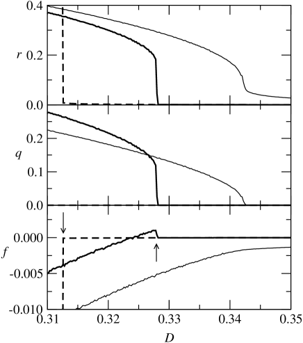
Figure 2: Order parameters $r$ and $q$ and free energy per site $f$ as functions of $D$, for $c=8.0$, exhibiting a continuous transition at $T=0.07$ (light solid lines) and a first-order transition at $T=0.04$ (heavy solid lines for SG states and dashed lines for P states) discussed in the text. The arrows indicate points on the spinodals.

Specific examples of results for the dependence of the order parameters with $D$ near the transition between the SG and the P phase obtained from Eqs. (26) and (27), that were used to construct the phase boundaries are shown in Fig. 2 for connectivity $c=8.0$ and two typical situations, one of the higher and the other one of the lower temperature behavior in which $T=0.07$ and $T=0.04$, respectively. The corresponding free energy for both situations, obtained by means of Eqs. (30) and (31), is shown in the lower panel of that figure. Each point on the curves is a result of an average over ten runs of the population dynamics procedure, in order to smooth out fluctuations. In the presence of multiple solutions for the parameters, we follow previous works on the fully connected model and choose the largest one in magnitude, that yields the lowest free energy which can be smoothly continued from one phase to the other with a change in $D$. The curves in Fig. 2 are rather close to those obtained already with a lower resolution, say $n=64$ and $N=10\,000$, indicating that the dynamics is near convergence. To test this point we found that further results for $r$, $q$ and $f$ obtained with $n=256$ and $N=160\,000$ at $T=0.04$, which is the case where the transition is first-order, are almost indistinguishable from those in Fig. 2.

As $D$ increases for $T=0.07$, $q$ and $r$ decrease continuously and the transition from the SG to the P phase takes place at $q=0$ and small $r$. When $T=0.04$, instead, there is a genuine first-order transition signalled by a continuous free energy with a discontinuity of the entropy and the appearance of a pair of spinodals, one for states (in solid lines) attained from the spin-glass phase and the other one for states (in dashed lines) reached from the paramagnetic phase with increasing or decreasing values of $D$, respectively. The arrows indicate the points on the spinodals for that value of $T$, and the transition between the phases appears at the crossing of the free energies, where $D=0.328$. The first-order transition persists for somewhat higher $T$ with the spinodals becoming closer up to the merging with the continuous transition at a tricritical point given by $T\simeq 0.059$ and $D\simeq 0.33$ for $c=8.0$, and similar results are obtained for other values of $c\geq c^{*}$ where $c^{*}$ is between $5.6$ and $6.0$, whereas only a continuous transition appears for smaller $c$ at all $T$. It is interesting to note that the changeover from a continuous to a discontinuous transition at low $T$ is preceded by a discontinuous transition between two SG states within the SG phase for $c^{*}\simeq 5.6$. For $c$ slightly larger this transition merges with the continuous transition that separates the two phases.

  

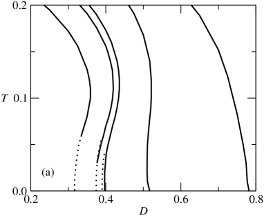
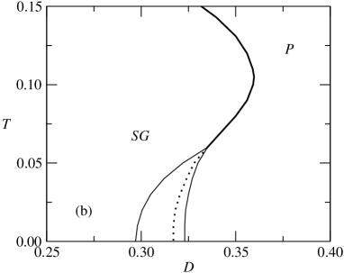
Figure 3: (a) The $T$ vs. $D$ phase diagram for connectivity $c=2.0$, $4.0$, $5.6$, $6.0$ and $8.0$ from right to left. Solid (dotted) lines denote continuous (discontinuous) transitions between a spin glass (SG) phase at left and a paramagnetic (P) phase at right of each curve. (b) Detail of the phase boundary for $c=8$ including the spinodals of the P and SG phases on the left and right of the transition in light solid lines, respectively.

A global picture of the transitions for finite connectivity is given by the $T$ vs. $D$ phase diagram for several values of $c\leq 8.0$ shown in Fig. 3. The transition is continuous for low $c$ and all $T$ with the order parameters going continuously to zero with increasing values of $D$, and there is a reentrance for $c\gtrsim 3.5$. On the other hand, a first-order transition appears with increasing $c$ between $5.6$ and $6.0$ at low but finite $T$ that starts at a tricritical point on the reentrance of the continuous phase boundary. The reentrance separates the P phase at low $T$ from the SG phase at higher $T$. Note that the tricritical point appears at larger values of $T$ with increasing $c$, and this has been checked by further calculations for $c=16$. We also found that, for all the values of $c$ larger than $\sim 2.5$ considered in this work, the phase boundaries move to the left with increasing $c$ towards lower values of $D$. Indeed, there is a monotonic decrease of $T_{0}(c)$, which is the critical $T$ at $D=0$, with increasing $c$ and we found numerically that $T_{0}\sim J/\sqrt{c}$ for large $c$, which is the same behavior as that in the two-state spin-glass model with finite connectivity where the transition is always continuous NC04 .

The reentrance of the phase boundaries is a manifestation of inverse freezing which appears either as a genuine first-order transition with a discontinuity of the entropy or as a continuous transition with only a gradual change in the entropy from one phase to the other. In order to show that the discontinuity of the entropy across the first-order transition in the GS model with finite connectivity goes in the right direction to account for inverse freezing we show in Fig. 4 (a) the temperature dependence of the free energy for $c=8$ and $D=0.325$. The free energy is continuous and follows the lower curve when there are two solutions and, indeed, the entropy of the P phase below the first-order transition (which is slightly positive for that value of $D$) is smaller than the entropy of the higher temperature SG phase, with a discontinuity of the entropy at the transition. This means that in heating the system the disordered paramagnet "freezes" into the amorphous SG with an exchange of latent heat. For comparison, we show in Fig. 4 (b) the free energy, for $D=0.35$, with no discontinuity in the entropy across the continuous transition.

The phase diagram for finite $c$ obtained in the present work within the RS scheme differs from the $T$ vs. $D$ phase diagram for the fully connected GS model in that, apparently, there is no reentrance in the latter within that scheme but there is a reentrance within full replica symmetry breaking. The first-order transition line appears in that case all along the reentrance of the phase boundary down to $T=0$ and it is even slightly continued above into the normal phase boundary. Thus, there is no continuous transition on the reentrance in that case. On the other hand there is, apparently, a further reentrance on the first-order transition at low $T$ CL05 .

The kind of behavior we find here for finite $c$ is similar to the phase diagram of a somewhat different model of a three-state Ising spin glass with full connectivity in which the degeneracy of the active spins ($\sigma=1$ or $\sigma=-1$) is larger than the degeneracy of the inactive state ($\sigma=0$), in contrast to the GS model where these degeneracies are the same. Indeed, the $T$ vs. $D$ phase boundary in that case also displays both a first-order transition at low $T$ and a continuous transition at higher $T$ on the reentrance of the phase boundary, even within the RS scheme SS03 .

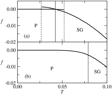
Figure 4: Temperature dependence of the free energy for $c=8$ across the first-order transition at $D=0.325$ in (a) and the continuous transition at $D=0.35$ in (b). The dashed left (right) line indicates a point on the SG (P) spinodals, respectively, and the vertical solid lines indicate the transition with an increase in entropy from the P to the SG phase in (a) and with no increase in (b). The normal transition between the SG and the P phase, not shown in the figure, appears at higher $T$.

Summary and conclusions

The statistical mechanics of the binary Ising SG model with finite random connectivity, within mean-field theory, has been extended in this work to study the three-state Ising SG model with crystal-field effects of Ghatak and Sherrington, which is a random-bond Blume-Capel model. Renewed interest in this model is due to the recent discovery of numerous physical realizations within condensed-matter physics that exhibit inverse transitions (see ref. PL10 for a recent review), and finite connectivity could be of use in order to study the behavior of such systems with effective interactions between infinite and short range or between infinite dimensions and three-dimensions.

The replica method for disordered spin systems with finite connectivity has been extended here within the replica symmetry (RS) ansatz. The RS ansatz for the order function that describes the behavior in the present model with finite connectivity introduces a distribution of a two-component effective field which plays a crucial role in determining the relevant order parameters of the model. An iterative self-consistency relation is derived for the local field distribution, an analytic solution of which does not seem possible in the presence of a first-order transition, and we use instead a population dynamics numerical procedure. Phase diagrams were then obtained in order to investigate the effects of finite connectivity and anisotropy parameter on the transitions between a SG and a P phase, with emphasis on reentrance behavior. The latter is a necessary feature in order to describe inverse transitions, in particular inverse freezing, in view of the two phases favored by the present model.

The main result of this paper is the $T$ vs. $D$ phase diagram, for various values of the connectivity, which exhibits the different phase transitions that may appear at low temperature. For low connectivity the transition is a continuous one down to $T=0$, with a reentrance at low $T$ for higher connectivity exhibiting both a continuous and a discontinuous transition. We showed that the discontinuous transition is a first-order transition with a discontinuity of the entropy at the transition in which the entropy of the SG phase is larger than the entropy of the P phase below the transition, which is a sign of inverse freezing in the system.

The results obtained so far within the RS ansatz could be changed by replica-symmetry breaking (RSB) and an extension in this direction could be interesting MP01 although not so easy to carry out in the present case due to the time consuming evaluation of the distribution of the two-dimensional effective field. However, if the trend of the results for the GS model with full connectivity are taken as a guide, one would expect an enhancement of the reentrance on the first-order transition for finite connectivity within RSB, without much change of the continuous transition.

It may also be interesting to find out to which extent the specific form of the distribution of random bonds makes a difference. In place of a Gaussian with mean zero and unit variance that we used in this work, one could have a Gaussian with mean $J_{0}>0$. We found that the phase diagram is somewhat changed in that case. Instead, one could consider a general bimodal distribution between ferromagnetic and antiferromagnetic interactions which allows to predict when the effects of frustration may become more relevant before going into a RSB calculation, an argument that has been used before NC04 . This, and related issues, are currently being studied.

The procedure extended in this work can be applied to study the effects of finite connectivity in other multi-state spin models like the random BEGC model or the degenerate spin model of Schupper and Shnerb either with random or uniform interactions SS03 ; CL05 . It can also be applied to attractor neural networks and the study of the retrieval performance in a three-state network with finite connectivity and a Hebbian learning rule is currently being investigated BET10 .

References

- (1) H. Nishimori, Statistical Physics of Spin Glasses and Information Processing (Oxford University Press, 2001).
- (2) D. Sherrington and S. Kirkpatrick, Phys. Rev. Lett. 35 1792 (1976).
- (3) M. Mezard, G. Parisi and M. A. Virasoro Spin Glass Theory and Beyond (World Scientific, Singapore, 1987).
- (4) T. Murayama, Y. Kabashima, D. Saad and R. Vicente Phys. Rev. E 62 (2000) 1577.
- (5) K. Nakamura, Y. Kabashima and D. Saad, Europhys Lett. 56 (2001) 610.
- (6) L. Viana and A. J. Bray, J. Phys. C: Solid State Phys. 18 (1985) 3037.
- (7) I. Kanter and H. Sompolinsky, Phys. Rev. Lett. 58 (1987) 164.
- (8) M. Mezard and G. Parisi, Europhys Lett. 3 (1987) 1067.
- (9) K. Y. Wong and D. Sherrington J. Phys. A: Math. Gen. 21 (1988) L459.
- (10) R. Monasson, J. Phys. A: Math. Gen. 31 (1998) 513.
- (11) M. Mezard and G. Parisi Eur. Phys. J. B 20 (2001) (217).
- (12) B. Wemmenhove and A. C. C. Coolen, J. Phys. A: Math. Gen. 36 (2003) 9617.
- (13) I. Perez Castillo and N. S. Skantzos, J. Phys. A: Math. Gen. 37 (2004) 9087.
- (14) I. Perez Castillo, B. Wemmenhove, J. P. L. Hatchett, A. C. C. Coolen, N. S. Skantzos and T. Nikoletopoulos, J. Phys. A: Math. Gen. 37 (2004) 8789.
- (15) T. Nikoletopoulos, A. C. C. Coolen, I. Perez Castillo, N. S. Skantzos, J. P. L. Hatchett and B. Wemmenhove, J. Phys. A: Math. Gen. 37 (2004) 6455.
- (16) A. Crisanti and L. Leuzzi, Phys. Rev. B 70, 014409 (2004).
- (17) A. Crisanti and L. Leuzzi, Phys. Rev. Lett. 95, 087201 (2005).
- (18) D. Bollé 2004 Advances in Condensed Matter and Statistical Mechanics ed E. Korutcheva and R. Cuerno (New York, Nova Science Publishers) p319.
- (19) S. K. Ghatak and D. Sherrington, J. Phys. C: Solid State Phys. 10 (1977) 3149.
- (20) F. A. da Costa, C. S. O. Yokoi and S. R. A. Salinas, J. Phys. A: Math. Gen. 27 (1994) 3365.
- (21) H. W. Capel, Physica (Amsterdam) 32, 966 (1966). M. Blume, Phys. Rev. 141, 517 (1966).
- (22) N. Schupper and N. M. Shnerb, Phys. Rev. Lett. 93 037202 (2004); Phys. Rev. E 72 046107 (2005).
- (23) M. Paoluzzi, L. Leuzzi and A. Crisanti, Phys. Rev. Lett. 104, 120602 (2010).
- (24) D. Bollé, R. Erichsen Jr and W. K. Theumann (in progress).