Cyclic Spectral Analysis of Radio Pulsars

Abstract

Cyclic spectral analysis is a signal processing technique designed to deal with stochastic signals whose statistics vary periodically with time. Pulsar radio emission is a textbook example of this signal class, known as cyclostationary signals. In this paper, we discuss the application of cyclic spectral analysis methods to pulsar data, and compare the results with the traditional filterbank approaches used for almost all pulsar observations to date. In contrast to standard methods, the cyclic spectrum preserves phase information of the radio signal. This feature allows us to determine the impulse response of the interstellar medium and the instrinsic, unscattered pulse profile directly from a single observation. We illustrate these new analysis techniques using real data from an observation of the millisecond pulsar B1937+21.

1 Introduction

Pulsar radio emission produces some of the most information-rich signals found in astronomy. Variation exists over a wide range of time scales, from ns-duration giant pulses (Hankins et al., 2003), to tiny decade-scale timing fluctuations that may eventually result in the first direct detection of gravitational radiation (Hobbs et al., 2010). Propagation of the radio pulses through the ionized interstellar medium (ISM) adds another layer of wavelength-dependent complexity (and information), including dispersion, multi-path scattering, and diffractive and refractive scintillation (Rickett, 1990). These effects provide a unique tool for exploring the structure of the ionized ISM in our galaxy on a wide range of scales. However, they also represent a still not fully understood source of systematic error for high-precision pulsar timing projects (Hemberger & Stinebring, 2008; Coles et al., 2010).

The complexity of the pulsar signal has led to the invention of a variety of specialized signal processing techniques. Currently, the most common approach to pulsar signal analysis is to divide the digitally-sampled baseband voltage into a number of frequency channels using a fast Fourier transform (FFT) or autocorrelation. The signal power is then detected in each channel, and integrated over a short time to produce a power spectrum estimate. This results in well-known tradeoffs and limitations on time and frequency resolution due to the competing effects of dispersive smearing and inverse channel bandwidth (Lorimer & Kramer, 2004). A major breakthrough came with the introduction of coherent dedispersion (Hankins & Rickett, 1975), in which a filter is applied within each channel pre-detection to completely remove the effect of dispersion, for a known dispersion measure (DM). This allows wider channels and hence higher time resolution to be achieved, and is commonly used for high-precision pulsar timing (e.g., Hotan et al., 2006; Demorest, 2007). This method is still bound by the fundamental time/frequency resolution relationship $\Delta t\Delta\nu\gtrsim 1$, with the values of $\Delta t$ and $\Delta\nu$ fixed at the time of observation.

Traditional spectral estimation procedures are based on an implicit assumption that the input signal is stationary, or at least approximately so over the spectrum integration timescale. However, the pulsar radio signal can be more accurately described as cyclostationary – it is a non-stationary random signal whose statistical properties vary periodically with time (Rickett, 1975). Over the past 20 years, statistical analysis techniques have been developed specifically to deal with cyclostationary signals, the study of which is known as cyclic spectral analysis (see reviews by Gardner, 1991; Antoni, 2007). These methods examine not only power versus frequency as in conventional spectral analysis, but also the correlation between spectral components that arises in cyclostationary signals. Cyclostationarity has recently been explored in a radio astronomy context for the identification and removal of radio frequency interference (Feliachi, 2010). However, these methods have not previously been applied to the pulsar signal itself. Doing so provides access to signal content that is unreachable via standard methods, and opens the door to a variety of novel analysis techniques.

In this paper, we describe the theory and practice of applying cyclic spectral analysis techniques to pulsar data. Section 2 gives a brief overview of cyclic spectral analysis and introduces the primary quantity of interest, the cyclic spectrum and its Fourier transforms. In Section 3, we describe in detail how the cyclic spectrum can be computed for pulsar observations, and present an example using actual data. Finally, Section 4 shows how the pulsar cyclic spectrum can be used to measure and correct for ISM scattering, and discusses possible future applications of these methods.

2 Cyclostationarity and Cyclic Spectral Analysis

We begin with a brief overview of stochastic processes and spectral analysis, to establish terminology. This is followed by a introduction of the main features of cyclic spectral anlysis. The more rigorous treatments presented by Papoulis (2002) for stochastic processes and Gardner (1992) for cyclic spectra are useful references. While we frame the discussion in terms of continuous-time functions, the discretization of the following equations is straightforward.

2.1 Standard Spectral Analysis

A general stochastic signal, $x(t)$, can largely be characterized by its second-order statistics. In the time domain, these are correlations, defined here symmetrically:

$$C_{x}(t,\tau)=E\left\{x(t+\frac{\tau}{2})x^{*}(t-\frac{\tau}{2})\right\}$$ (1)

Here, the expectation value represents an average over many realizations of the signal. Stationary processes are those whose correlation function depends only on the time difference $\tau$ between any two points and not explicitly on the time $t$. While the signals themselves have random variation versus time, their statistics are constant. The signal can alternately be characterized by the power spectrum $S_{x}(\nu)$, which is the Fourier transform of the correlation function $C_{x}(\tau)$.

For ergodic signals, the correlation function can be estimated from a single realization of the signal via a time average:

$$C_{x}(\tau)=T^{-1}\int_{0}^{T}x(t+\frac{\tau}{2})x^{*}(t-\frac{\tau}{2})dt$$ (2)

This forms the basis for practical spectral analysis of random signals. In practice, both ergodicity and stationarity are almost always assumed a priori, since one usually has only one realization of a signal. Due to the Fourier-pair uncertainty relations, the spectral resolution $\Delta\nu$ is limited to approximately $T^{-1}$ or larger.

In radio astronomy, $x(t)$ is the baseband voltage, a quantity proportional to the incident radio wave’s electric field, mixed (frequency-shifted) to near zero frequency. Early digital radio spectrometers often explicitly evaluated Eqn. 2 using dedicated hardware. In modern systems, $S_{x}(\nu)$ is usually computed using a fast Fourier transform (FFT) of $x(t)$. In order for a pulse to be resolved in time, $T$ must be small compared to the pulse width. For pulsars, this puts a limit on the finest achievable frequency resolution of $\Delta\nu\gtrsim(P\Delta\phi)^{-1}$ where $P$ is the pulse period and $\Delta\phi$ is the pulse width in turns.

2.2 Cyclic Spectral Analysis

An interesting class of nonstationary signal are those whose statistics vary periodically with time. These are known as cyclostationary signals and their correlations exhibit periodicity:

$$C_{x}(t,\tau)=C_{x}(t+P,\tau)=C_{x}(t\bmod P,\tau)$$ (3)

It is important to note that although $C_{x}(t,\tau)$ is periodic in $t$, it is not generally periodic in $\tau$, and $x(t)$ itself is not necessarily a periodic function. Simple examples of cyclostationary signals can be obtained by periodically amplitude- or frequency-modulating a stationary noise process. In this paper we will sometimes use the quantity pulse phase $\phi=t/P$ in place of $t$ as an independent variable in expressions such as $C_{x}(\phi,\tau)$.

The cyclic analog of the power spectrum can be obtained by Fourier transforming $C_{x}(t,\tau)$ along both the $t$ and $\tau$ axes:

$$S_{x}(\nu;\alpha)=P^{-1}\int\limits_{-\infty}^{+\infty}d\tau\int\limits_{0}^{P}dt\;C_{x}(t,\tau)e^{-2\pi i\nu\tau}e^{-2\pi i\alpha t}$$ (4)

This quantity is known as the cyclic spectrum and it is a function of two frequency variables. The frequency $\nu$ is conjugate to $\tau$ exactly as in the standard power spectrum. The cycle frequency $\alpha$ is conjugate to $t$, and takes on the discrete values $\alpha_{n}=n/P$ – it is computed here as a Fourier series rather than a continuous Fourier transform. In the stationary signal case, $S_{x}(\nu;\alpha)=0$ for $\alpha\neq 0$.

The periodic correlation can be estimated from a single signal realization similarly to Eqn. 2 by “folding” the correlations modulo the periodicity $P$:

$$C_{x}(t,\tau)=N^{-1}\sum_{n=0}^{N}x(t+nP+\frac{\tau}{2})x^{*}(t+nP-\frac{\tau}{2})$$ (5)

This again assumes ergodicity of the signal, over $N$ periods. In this computation, the integration time $T$ is given by $NP$, the number of periods folded. The integration time sets an ultimate limit on the range of $\tau$ that can be measured, and again the spectral resolution is limited to $\Delta\nu\gtrsim T^{-1}$. However, in constrast with Eqn. 2, $T$ is not constrained by the pulse width, as the nonstationarity has already been correctly taken into account in Eqn. 5. This decouples the pulse phase resolution from the frequency resolution.

It is easy to see that various symmetry relationships exist among these quantities. In our symmetric formulation, $C_{x}(t,-\tau)=C^{*}_{x}(t,\tau)$. Similarly, $S_{x}(\nu;-\alpha)=S^{*}_{x}(\nu;\alpha)$. A useful intermediate quantity is the periodic spectrum $S_{x}(\nu,t)$ that is obtained by Fourier transforming $C_{x}(t,\tau)$ with respect to $\tau$ alone. By symmetry, $S_{x}(\nu,t)$ is purely real-valued, and therefore is straightforward to visualize. $S_{x}(\nu,t)$ is superficially similar to signal power as a function of time and frequency. However as discussed below, it also contains information about the signal phase, and thus is not strictly positive.

It can be shown that the cyclic spectrum also represents correlations in the frequency domain (Gardner, 1991, 1992). Using the Fourier transform of $x(t)$, $X(\nu)$, we have:

$$S_{x}(\nu;\alpha)=E\left\{X(\nu+\alpha/2)X^{*}(\nu-\alpha/2)\right\}$$ (6)

This relationship directly leads to a key result on which we will rely heavily in later sections: If $y(t)$ is the result of passing $x(t)$ through a linear, time-invariant filter with impulse response $h(t)$ (frequency response $H(\nu)$),

$$y(t)=h(t)\star x(t)$$ (7)

$$Y(\nu)=H(\nu)X(\nu)$$ (8)

then the cyclic spectra of $x$ and $y$ are related by:

$$S_{y}(\nu;\alpha)=H(\nu+\alpha/2)H^{*}(\nu-\alpha/2)S_{x}(\nu;\alpha)$$ (9)

Eqn. 9 shows that the phase content of $H(\nu)$ is preserved in the cyclic spectrum, whereas in a standard power spectrum the only information retained is the filter magnitude $\left|H(\nu)\right|^{2}$. This is a fundamental difference between the two approaches that will enable most of the novel applications described in §4.

In practice, computation of any of the cyclic spectrum variants will be done using band-limited, digitized sampled values. That is, the signal from the radio frequency of interest will be filtered with a bandpass filter of width $B$, mixed to baseband and critically sampled at the Nyquist rate. It is well known that any remaining power outside the baseband frequency range $-B/2<\nu<B/2$ will be aliased into the sampled values. Similar considerations applied to cyclic spectra show that the resulting $S(\nu;\alpha)$ is only valid within a diamond-shaped region around the origin, defined by $|\alpha/2|+|\nu|<B/2$.

3 Implementation for Pulsar Data

A simple but useful model of the pulsar radio signal $y(t)$ as it is received on Earth is amplitude-modulated noise (Rickett, 1975):

$$y(t;t_{0},\nu_{0})=h_{ISM}(t;t_{0})\star\left(p(t\Omega(t_{0});\nu_{0})n_{i}(t)\right)$$ (10)

Here, $n_{i}(t)$ is a stationary noise process representing the intrinsic pulsar radio emission. $p(\phi;\nu_{0})$ is a periodic function describing the average pulse profile shape at a radio frequency $\nu_{0}$. The timing model $\Omega(t_{0})$ gives the apparent rotational frequency of the pulsar at a given time. This includes the slowly-changing intrinsic spin frequency of the pulsar as well as Doppler and relativistic terms due to the motions of the Earth and pulsar. The impulse response function, $h_{ISM}(t;t_{0})$, describes the effect of the ionized interstellar medium (ISM) on the radio signal. It contains both dispersion and scintillation/scattering terms, and slowly evolves with a characteristic timescale $t_{d}$ due to the relative motions of the Earth, ISM, and pulsar. For clarity, we will often omit the slow dependences on $t_{0}$ and $\nu_{0}$ in the following discussion.

Under the approximation that the average intrinsic pulsar emission spectrum $S_{n}(\nu)=S_{0}$ is flat (valid over small fractional bandwidths), the pre-ISM pulsar cyclic spectrum takes the simple form $S_{x}(\nu;\alpha_{n})=I(n)S_{0}$, where $I(n)$ is the Fourier transform of the intensity profile $I(\phi)=\left[p(\phi)\right]^{2}$ and $\alpha_{n}=n\Omega$. The addition of the ISM filtering process produces an expression for the final pulsar cyclic spectrum:

$$S_{y}(\nu;\alpha_{n})=H_{ISM}(\nu+\frac{\alpha_{n}}{2})H^{*}_{ISM}(\nu-\frac{\alpha_{n}}{2})I(n)S_{0}$$ (11)

The duration of the ISM impulse response, $\tau_{ISM}$, can be approximated as the combination of the two primary effects, dispersion and scattering: $\tau_{ISM}^{2}\approx\tau_{DM}^{2}+\tau_{sc}^{2}$. In order to resolve the full frequency structure of $H_{ISM}(\nu)$, the cyclic spectra must be computed with a frequency resolution $\Delta\nu\lesssim(2\tau_{ISM})^{-1}$. Since $H_{ISM}(\nu)$ is slowly evolving with time, the cyclic spectrum integration time should be kept shorter than the diffractive scintillation timescale $t_{d}$ for the signal model presented in Eqn. 11 to apply.

3.1 Time-domain Approach

A time domain approach to computing the cyclic spectrum is based on directly evaluating Eqn. 5. In this method, the complex-conjugated baseband values are delayed by an integer number of samples (“lags”), and then multiplied by the original undelayed version. The pulse phase for each point in this cross-multiplied data stream is calculated using standard methods (polynomial expansion of $\Omega(t_{0})$) and then they are folded into the desired number of pulse phase bins. The process is repeated for the desired number of delays ($N_{lag}$). Due to symmetry, only positive lags need be evaluated. When combined with the “mirrored” negative lag values, the result is an $N_{bin}$ by $N_{chan}=2N_{lag}-1$ array representation of $C_{x}(\phi,\tau)$. This computation can be preceded by standard coherent dedispersion at a known DM to reduce the required frequency resolution, effectively setting $\tau_{DM}$ to $\sim 0$.

This time domain method has the benefit of straightforward handling of the relationship between the slowly changing pulse period and sampling rate. It also is easily integrated into standard pulsar observing practices: The “zero-lag” term is simply a standard folded pulse profile as would usually be computed by a traditional pulsar processing system. The drawback to this method is that the computational cost per sample scales linearly with $N_{chan}$, quickly becoming impractical if fine frequency resolution is desired. For real time computation over a total bandwidth $B$ with frequency resolution $\Delta\nu$, the computational cost in floating-point operations per second (flops) is given by

$$\mathcal{C}_{T}(B,\Delta\nu)\simeq 4N_{pol}\frac{B^{2}}{\Delta\nu}$$ (12)

Here, $N_{pol}$ equals 2 if only total power terms are computed, or 4 if polarization cross-products are included. An implementation of the time-domain cyclic spectrum method is now included in the open-source DSPSR software package (van Straten & Bailes, 2010).

3.2 Frequency-domain Approach

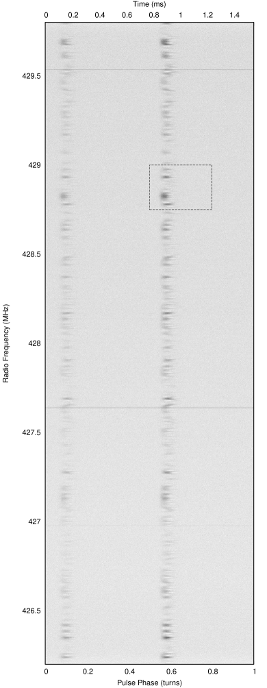
Figure 1: Periodic spectrum $S_{x}(\nu,t)$ of B1937+21 using frequency resolution of $4~{}\mathrm{MHz}/6320=0.642~{}\mathrm{kHz}$ and pulse phase resolution of $1.55~{}\mathrm{ms}/511=3~{}\mu\mathrm{s}$. The boxed region is shown in detail in Figure 2.

It is also possible to compute the cyclic spectrum in the frequency domain, based on Eqn. 6. In this method, the raw samples are first Fourier transformed with resolution determined by the $\tau_{ISM}$ timescale. The frequency domain data is multiplied by an appropriate phase gradient to align the data in pulse phase, and a coherent dedispersion filter is optionally applied at this point. The frequency domain correlations of Eqn. 6 are then computed for $N_{lag}^{\prime}$ “spectral lags” of spacing $\alpha_{n}$. The number of spectral lags determines the pulse phase resolution, with $N_{bin}=2N_{lag}^{\prime}-1$. However, since there is generally not an integer number of pulse periods per FFT length, the frequencies required for evaluating Eqn. 6 fall between FFT bins. In order to avoid artifacts in the resulting cyclic spectra, the FFT output must be interpolated to obtain the correct fractional frequencies. Here we use a 7-point sinc interpolation with good results and leave a detailed study of the effect of this interpolation for future work. Finally the correlations are averaged into $N_{chan}$ frequency bins. As in the time domain case, applying coherent dedispersion reduces the final required frequency resolution.

The frequency domain method has the advantage of the computational requirements scaling linearly with $N_{bin}$ rather than $N_{chan}$ as in the time domain version. This is attractive for situations where very fine frequency resolution is desired. However, there is some added complexity due to the frequency interpolation, and this method is a much larger departure from standard pulsar observing strategies. For this method, the number of flops required for real-time computation is

$$\mathcal{C}_{F}(B,\Delta\nu)\simeq N_{bin}(2N_{int}+4N_{pol})B+5B\log_{2}\frac{B}{\Delta\nu}$$ (13)

where $N_{int}$ is the number of points in the interpolation kernel. The second term is the approximate cost of the initial FFT. Real-world FFT performance can depart significantly from this scaling depending on the implementation details and computing hardware architecture.

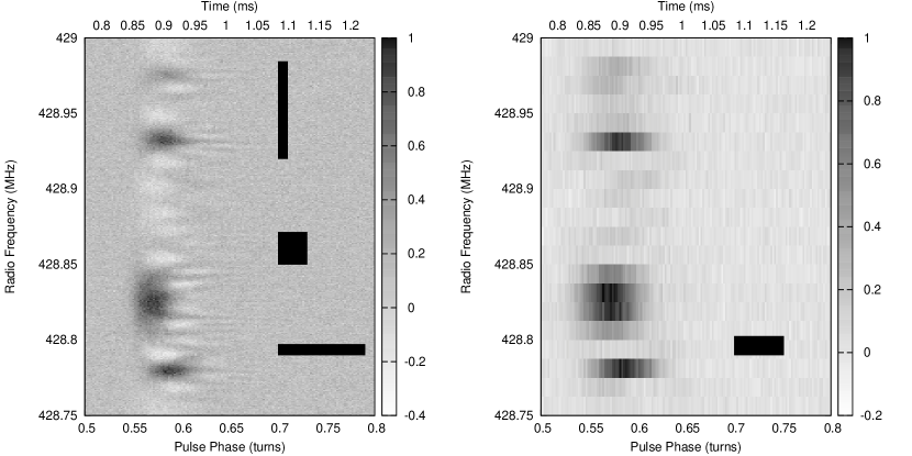
Figure 2: Left: Detail of periodic spectrum of B1937+21. The black rectangles each contain unity time-frequency area. The fixed resolution implied by any one of these, as is produced by a traditional filterbank, would miss various features in the data. Note also the appearance of both positive (dark) and negative (light) signal regions at fine scales. This is due to the phase content of $H_{ISM}(\nu)$ present in this representation. Right: The same data processed with a standard coherently dedispersed filterbank (DSPSR; van Straten & Bailes, 2010), using a frequency resolution of 12.5 kHz, and corresponding intrinsic time resolution of 80 $\mu$s (black rectangle). The data are oversampled in pulse phase by a factor of $\sim$20, resulting in the same number of profile bins as in the left panel. In both panels the zero-point has been determined by measuring the mean off-pulse level, and the data have been normalized by the peak value.

3.3 Hybrid Filterbank Methods

Neither the time-domain method of Section 3.1 or the frequency-domain method of Section 3.2 is efficient for direct application to a wide ($B\gtrsim 10$ MHz) frequency band. $\mathcal{C}_{T}$ scales as $B^{2}$, and while $\mathcal{C}_{F}$ formally grows only as $B\log B$, the FFT length required for dedispersion grows as $B^{2}$ and eventually becomes impractical in current computing hardware. The computational burden can be reduced by first splitting the wide band into a number of sub-bands via a filterbank, and then applying either the time or frequency domain cyclic spectrum computation method in each sub-band separately. This is similar to how most coherent dedispersion algorithms currently work. However, in contrast with standard filterbanks, to compute a continuous cyclic spectrum over the full wide band, the sub-bands must be made to overlap in frequency. As explained at the end of Section 2.2, the cyclic spectrum can not be properly computed for frequencies within $\alpha/2$ of an edge of a band-limited signal. Therefore to avoid gaps at each sub-band edge, the sub-bands must overlap by an amount $B_{ol}\geq\alpha_{max}$, and the invalid edges discarded before finally appending the sub-band results together. This approach results in a total number of real-time flops given by

$$\mathcal{C}_{H}\simeq\mathcal{C}_{FB}(B,B_{s})+\frac{B}{B_{s}-B_{ol}}\mathcal{C}_{T,F}(B_{s},\Delta\nu)$$ (14)

where $\mathcal{C}_{FB}$ is the cost of the filterbank operation, $B_{s}$ is the full width of each sub-band (including the overlapped portion), and $\mathcal{C}_{T,F}$ is the cost of either of the previously explained methods applied to a single sub-band. Due to the relationship $B_{s}>B_{ol}\geq\alpha_{max}$, the minimum possible sub-band width is set by the desired pulse phase resolution $\Delta\phi=(2P\alpha_{max})^{-1}$.

3.4 Example Data

We illustrate the concepts just discussed with an example of cyclic spectrum computation on actual pulsar data. We observed the 1.55-ms pulsar B1937+21 at Arecibo Observatory using the Astronomy Signal Processor (ASP) pulsar backend (Demorest, 2007). Dual-polarization, 8-bit baseband voltage samples were recorded in a 4 MHz band centered on 428 MHz. Cyclic spectra were computed via the frequency domain method discussed in §3.2 using a FFT length of 542288 points, 256 spectral lags and integrated for $T_{int}=2$ minutes. The FFT length was chosen based on the dispersion time $\tau_{DM}\sim 30$ ms. A coherent dedispersion filter using a DM of 71.019 pc cm^-3 was applied before summing the cyclic spectra to the final output frequency resolution of $N_{chan}=6230$ ($\Delta\nu=0.642$ kHz). When transformed to the periodic spectrum domain (Figures 1 and 2), the 256 harmonics result in $N_{bin}=511$ ($P\Delta\phi=3.0$ $\mu$s). The spectra were computed separately for each polarization, then summed to make the total intensity spectrum shown. For this example, the radio frequency resolution $\Delta\nu$ was chosen to be approximately equal to $1/P$, providing equal spacing between points in the $\nu$ and $\alpha$ dimensions in the cyclic spectrum.

PSR B1937+21 is an ideal case for showing the utility of these methods. Near 430 MHz, the typical ISM scattering time is $\tau_{sc}\sim 40~{}\mu\mathrm{s}$, comparable to the intrinsic pulse width (Cordes et al., 1990). Even if coherent dedispersion is first performed, the typical filterbank approach forces one to choose between: 1. Resolving the scintillation structure (on frequency scales $\sim\tau_{sc}^{-1}$) but losing almost all pulse shape information; or 2. Retaining enough time resolution to resolve the pulse, but missing most of the fine frequency structure. These tradeoffs are graphically illustrated in Figure 2, where it can be seen that the cyclic spectrum approach retains information on both small pulse phase and frequency scales. As previously mentioned, the periodic spectrum contains signal phase information and the on-pulse region can be seen to contain both positive and negative components, relative to the mean off-pulse level. Also notable are the fine “streaks” that appear at later pulse phases. One possible explanation for these features is that in this part of the profile the signal is dominated by more highly delayed components, making the periodic correlation $C(\phi,\tau)$ contain signal power at larger $|\tau|$ values than are present at earlier phases. When transformed to the periodic spectrum domain, this results in finer frequency structure appearing at later pulse phases.

4 Applications

Given the signal model presented in Eqn. 11, it is possible to determine both the ISM response and intrinsic pulse profile directly from a single cyclic spectrum. The two-dimensional cyclic spectrum $S(\nu;\alpha_{n})$ contains $N_{chan}\times N_{lag}^{\prime}$ data values, while $H_{ISM}(\nu)$ and $I(n)$ are described by only $N_{chan}+N_{lag}^{\prime}$ model parameters. This provides sufficient constraints for both to be determined via iterative least-squares minimization. A detailed analysis of this method will be presented in a separate paper (Walker et al., 2011). One previous measurement method for $h_{ISM}(t)$ has been published (Walker et al., 2008), based on a dynamic spectrum phase retrieval procedure. The cyclic spectrum method is much simpler since in this case the wave phases can be measured directly, giving an estimate of $h_{ISM}$ from a single “snapshot” observation. The cyclic spectrum also incorporates pulse profile shape information, which is lost in standard dynamic spectra. This naturally leads, for the first time, to a true coherently descattered pulse profile shape (Figure 3). In contrast with previous intensity-based profile deconvolution methods (Bhat et al., 2004), this requires no assumption of a specific functional form for $h_{ISM}$ and is not affected by ambiguity between intrinsic and ISM-induced profile features. The ISM response shown in Figure 3 has an initial exponential decay followed by a more slowly-decaying tail. This will be interesting to compare in detail with the predictions of the standard Kolmogorov scattering model (e.g., Rickett et al., 2009).

There are several degeneracies that the descattering process alone can not resolve. As is clear from Eqn. 11, multiplying $H_{ISM}$ by a constant phase factor will produce no change in the observed cyclic spectrum. Similarly, without additional assumptions, the pulsar’s intrinsic flux $S_{0}$ is degenerate with the magnitude of $H_{ISM}$. Most critically for pulsar timing, an arbitrary rotation can be applied to $I(\phi)$, and absorbed into $H_{ISM}$. That is, at this level of analysis it is impossible to distinguish an ISM-induced delay from a pulsar spin deviation or other timing effect. Resolving this situation to obtain properly scattering-corrected timing will require the development of additional analysis techniques. This could range from assuming a constrained form or applying moment analysis to $h_{ISM}$ to physical models of the spatial distribution of scattering material, and is an active topic for further study. Compared with previous methods, the cyclic spectrum provides a qualitatively new way to measure the ISM response, and this new information dramatically expands the possibilities for scattering corrections to timing data.

In addition to the determination of $H_{ISM}$, Eqn. 9 allows for the applcation of other phase-coherent filters to the final integrated cyclic spectra. This technique can be used to perform coherent dispersion corrections, within the limits of the cyclic spectrum resolution. The high frequency resolution of the pulsar cyclic spectrum enables precise post-detection removal of narrow-band radio frequency interference, without sacrificing pulse phase resolution. More sophisticated approaches may also incorporate information gained from the cyclostationarity of the interference (Feliachi, 2010).

Although the discussion in §2 focused on the analysis of a single stochastic signal, pairs of correlated cyclostationary signals can be analyzed via cyclic cross-spectra, in complete analogy with standard cross-spectra (Gardner, 1992). For dual-polarization radio data, this results in the creation of cyclic Stokes parameters, and allows for the application of phase-coherent matrix convolution (van Straten, 2002) directly to the cyclic spectra. For radio interferometers, analyzing data from antenna pairs will produce cyclic visibilities. Along with recently developed VLBI imaging techniques for investigating pulsar scintillation (Brisken et al., 2010), this could prove to be an extremely powerful tool for exploring the ISM.

Figure 3: Top: Absolute square of the impulse response $|h_{ISM}(t)|^{2}$ determined from the data shown in Figure 1. Bottom: Corresponding standard (dashed) and scattering-corrected (solid) pulse profiles. All functions have been normalized by their peak value. The x-axis range covers the same total time span in both panels.

5 Conclusions

Cyclic spectral analysis is a powerful new observational technique for studying radio pulsars. It provides a data representation that simultaneously preserves both high pulse phase resolution and high frequency resolution information about the signal. With the accompanying preservation of signal phase content, this allows fundamentally new analysis techniques not possible with standard filterbank data. This holds promise both for increasing our understanding of the ionized ISM, and eventually for removing ISM scattering as an obstacle to achieving the highest possible pulsar timing precision.

References

- Antoni (2007) Antoni J., 2007, Mechanical Systems and Signal Processing, 21, 597
- Bhat et al. (2004) Bhat N. D. R., Cordes J. M., Camilo F., Nice D. J., Lorimer D. R., 2004, ApJ, 605, 759
- Brisken et al. (2010) Brisken W. F., Macquart J., Gao J. J., Rickett B. J., Coles W. A., Deller A. T., Tingay S. J., West C. J., 2010, ApJ, 708, 232
- Coles et al. (2010) Coles W. A., Rickett B. J., Gao J. J., Hobbs G., Verbiest J. P. W., 2010, ApJ, 717, 1206
- Cordes et al. (1990) Cordes J. M., Wolszczan A., Dewey R. J., Blaskiewicz M., Stinebring D. R., 1990, ApJ, 349, 245
- Demorest (2007) Demorest P. B., 2007, PhD thesis, University of California, Berkeley
- Feliachi (2010) Feliachi R., 2010, PhD thesis, Université d’Orléans, France
- Gardner (1991) Gardner W., 1991, Signal Processing Magazine, IEEE, 8, 14
- Gardner (1992) Gardner W. A., 1992, Statistical Signal Analysis: A Non-probabilistic Theory
- Hankins et al. (2003) Hankins T. H., Kern J. S., Weatherall J. C., Eilek J. A., 2003, Nature, 422, 141
- Hankins & Rickett (1975) Hankins T. H., Rickett B. J., 1975, in Methods in Computational Physics. Volume 14 - Radio astronomy Pulsar signal processing. pp 55–129
- Hemberger & Stinebring (2008) Hemberger D. A., Stinebring D. R., 2008, ApJ, 674, L37
- Hobbs et al. (2010) Hobbs G., et al., 2010, Classical and Quantum Gravity, 27, 084013
- Hotan et al. (2006) Hotan A. W., Bailes M., Ord S. M., 2006, MNRAS, 369, 1502
- Lorimer & Kramer (2004) Lorimer D. R., Kramer M., 2004, Handbook of Pulsar Astronomy. Cambridge University Press
- Papoulis (2002) Papoulis A., 2002, Probability, Random Variables and Stochastic Processes
- Rickett et al. (2009) Rickett B., Johnston S., Tomlinson T., Reynolds J., 2009, MNRAS, 395, 1391
- Rickett (1975) Rickett B. J., 1975, ApJ, 197, 185
- Rickett (1990) Rickett B. J., 1990, ARA&A, 28, 561
- van Straten (2002) van Straten W., 2002, ApJ, 568, 436
- van Straten & Bailes (2010) van Straten W., Bailes M., 2010, ArXiv e-prints
- Walker et al. (2011) Walker M. A., Demorest P. B., van Straten W., 2011, in prep
- Walker et al. (2008) Walker M. A., Koopmans L. V. E., Stinebring D. R., van Straten W., 2008, MNRAS, 388, 1214