Long-Term Cycling of Kozai-Lidov Cycles: Extreme Eccentricities and Inclinations Excited by a Distant Eccentric Perturber

Abstract

Kozai-Lidov oscillations of Jupiter-mass planets, excited by comparable planetary or brown dwarf mass perturbers were recently shown in numerical experiments to be slowly modulated and to exhibit striking features, including extremely high eccentricities and the generation of retrograde orbits with respect to the perturber. Here we solve this problem analytically for the case of a test particle orbiting a host star and perturbed by a distant companion whose orbit is eccentric and highly inclined. We give analytic expressions for the conditions that produce retrograde orbits and high eccentricities. This mechanism likely operates in various systems thought to involve Kozai-Lidov oscillations such as tight binaries, mergers of compact objects, irregular moons of planets and many others. In particular, it could be responsible for exciting eccentricities and inclinations of exo-planetary orbits and be important for understanding the spin-orbit (mis)alignment of hot Jupiters.

A Keplerian orbit weakly perturbed by a distant orbiting mass may exhibit long term, large amplitude cycles in which the eccentricity and inclination change periodically Lidov (1962); Kozai (1962). These so-called Kozai-Lidov cycles are owed to the orbit-averaged quadrupole potential of the perturber. The high eccentricity excited from initially nearly circular orbits by this mechanism is suggested to play an important role in the formation and evolution of many astrophysical systems (e.g. Kozai, 1962; Heisler & Tremaine, 1986; Blaes et al., 2002; Fabrycky & Tremaine, 2007; Perets & Naoz, 2009; Thompson, 2010; Naoz et al., 2011).

Kozai-Lidov oscillations of Jupiter-mass planets, excited by comparable planetary or brown dwarf mass perturbers were recently shown in numerical experiments to be slowly modulated and to exhibit striking features, including extremely high eccentricities and the generation of retrograde orbits with respect to the perturber Naoz et al. (2011) (see also Ford et al. (2000)). Those authors attributed the slow modulation of the Kozai-Lidov cycles to the relative proximity (including the octupole potential of the perturber) and comparable mass of the perturber to the perturbed planet, and the high eccentricities to chaotic evolution. These effects were argued to play a major role in affecting the properties of hot Jupiters (extra-solar, Jupiter mass planets with very short periods $\lesssim$ 10 days) and in particular in explaining the large fraction of hot Jupiters recently found to have a retrograde orbit with respect to their host’s spin.

In this letter we show that the Kozai-Lidov cycles are slowly modulated non-chaotically and quite simply by the octupole potential of the perturber, which is non-vanishing when the perturber’s orbit is eccentric. This slow modulation can excite extremely high eccentricity and inclination of an initially nearly circular Keplerian orbit. A particular consequence is that the orbit plane can flip to retrograde with respect to the total angular momentum of the system Naoz et al. (2011). These effects occur in the test particle approximation in which the mass of the perturber is much bigger than that of the planet, and will thus be important for stellar binary perturbers of planets. We describe this long term evolution of the Kozai-Lidov cycles by deriving and analytically solving the effective equations, averaged over the Kozai cycles.

Secular Equations

Consider a test particle on a Keplerian orbit (semi-major axis $a$ and eccentricity $e$) subject to perturbation by a distant mass $M_{\text{per}}$ on an orbit ($a_{\text{per}}$, $e_{\text{per}}$) around the same central mass $M$. The coordinate system is defined using the perturber’s orbit, with the z-axis chosen to be in the direction of the angular momentum vector and the x-axis pointing to the pericenter. It is useful to parametrize the test particle’s orbit by two dimensionless vectors: $\textbf{j}=\mathbf{J}/\sqrt{GMa}$, where $\mathbf{J}$ is the specific angular momentum vector and $G$ is the universal constant of gravitation; e, a vector pointing in the direction of the pericenter with magnitude $e$. The orientation of j is defined by the inclination $i$ with respect to $\hat{\textbf{z}}$ and by the longitude of ascending node $\Omega$ (angle between $\hat{\textbf{z}}\times\textbf{j}$ and $\hat{\textbf{x}}$), as follows ${\textbf{j}=j(\sin i\sin\Omega,~{}-\sin i\cos\Omega,~{}\cos i).}$ Usually, the orientation of e is set by additionally specifying the argument of pericenter $\omega$ (angle between e and $\hat{\textbf{z}}\times\textbf{j}$). Here we define the orientation of e by the co- latitudinal angle $0\leq i_{e}\leq\pi$ (angle between $\hat{\textbf{z}}$ and e), and longitude $\Omega_{e}$ (angle between the projection of e on the $xy$ plane and $\hat{\textbf{x}}$) by

$$\textbf{e}=e(\sin i_{e}\cos\Omega_{e},~{}\sin i_{e}\sin\Omega_{e},~{}\cos i_{e}).$$ (1)

It turns out that for the cases considered, $\Omega_{e}$ is slowly varying and is useful for describing the long term behavior of the system.

The secular orbital evolution of the test particle is determined by double time-averaging the perturbing potential $\Phi_{\text{per}}$ over the orbital periods of the test particle and the perturber. The averaged potential expanded to the octupole order (3rd order in $a/a_{\text{per}}$) is given by $\left\langle\Phi_{\text{per}}\right\rangle=\Phi_{0}\phi=\Phi_{0}(\phi_{\text{Quad}}+\epsilon_{\text{Oct}}\phi_{\text{Oct}})$, where the dimensionless averaged potential $\phi$ is expressed as the sum of two components (quadrupole and octupole),

$$\phi_{\text{Quad}} = \frac{3}{4}(\frac{1}{2}j_{z}^{2}+e^{2}-\frac{5}{2}e_{z}^{2}-\frac{1}{6}),$$ (2)

$$\phi_{\text{Oct}} = \frac{75}{64}\left[e_{x}(\frac{1}{5}-\frac{8}{5}e^{2}+7e_{z}^{2}-j_{z}^{2})-2e_{z}j_{x}j_{z}\right],$$ (3)

and the normalization parameters are

$$\Phi_{0}=\frac{GM_{\text{per}}a^{2}}{{a_{\text{per}}^{3}{(1-e_{\text{per}}^{2}})}^{3/2}},~{}~{}~{}~{}\epsilon_{\text{Oct}}=\frac{a}{a_{\text{per}}}\frac{e_{\text{per}}}{1-e_{\text{per}}^{2}}.$$ (5)

In the secular approximation, $a$ and $\phi$ are constant with time while j and e evolve according to the following equations of motion Milankovich (1939); Allan & Ward (1963); Tremaine et al. (2009),

$$\frac{d\textbf{j}}{d\tau}=\textbf{j}\times\nabla_{\textbf{j}}\phi+\textbf{e}\times\nabla_{\textbf{e}}\phi,~{}~{}~{}\frac{d\textbf{e}}{d\tau}=\textbf{j}\times\nabla_{\textbf{e}}\phi+\textbf{e}\times\nabla_{\textbf{j}}\phi,$$ (6)

where $\tau=t/t_{\rm sec}$ and $t_{\rm sec}={\sqrt{GMa}}/{\Phi_{0}}$ is the secular timescale. Physical solutions are restricted to those satisfying the physical constraints $j^{2}=|\textbf{j}|^{2}=1-e^{2},$ and $\textbf{e}\cdot\textbf{j}=0$.

Kozai-Lidov Cycles

When expanded to the quadrupole order only (i.e., $\epsilon_{\text{Oct}}=0$), the averaged perturbing potential is axisymmetric. As a consequence, $j_{z}$ is conserved and the equations of motion are invariant under rotational transformations around the $z$ axis. In this case, $e$, $i$, $\omega$ and $i_{e}$ undergo periodic oscillations (Kozai-Lidov cycles), which are determined by the two constants of motion $j_{z}$ and $\phi=\phi_{\text{Quad}}$ (e.g. Lidov, 1962; Kozai, 1962). It is convenient to use the constant of motion $C_{K}=\frac{4}{3}\phi_{\text{Quad}}-\frac{1}{2}j_{z}^{2}+\frac{1}{6}$, which is given by

$$C_{K}=e^{2}-\frac{5}{2}e_{z}^{2}=e^{2}(1-\frac{5}{2}\sin^{2}i\sin^{2}\omega).$$ (7)

When $C_{K}<0$, $\omega$ librates around $\pi/2$ or $-\pi/2$ (Kozai-Lidov librations), while for $C_{K}>0$, $\omega$ varies monotonically with time taking all values from $0$ to $2\pi$ (Kozai-Lidov rotations).

For rotations, $e$ reaches minimum at $\omega=0$ or $\pi$, implying

$$e_{\min}^{2}=C_{K}~{}~{}~{}~{}~{}(\text{only when}~{}C_{K}>0).$$ (8)

For librating solutions, $e_{\min}$ is obtained at $\omega=\pm\pi/2$. For any Kozai-Lidov cycle, maximum $e$ is obtained at $\omega=\pm\pi/2$, leading to

$$3e^{4}_{\max}+(5j_{z}^{2}-3+2C_{K})e^{2}_{\max}-2C_{K}=0.$$ (9)

To fully specify the trajectory, the azimuthal position must be specified. We use the azimuthal angle $\Omega_{e}$, which, as shown below changes slowly for the regime $j_{z}^{2}\ll 1$ of interest here. In fact, the equation of motion for $\Omega_{e}$ reads

$$\dot{\Omega}_{e}=j_{z}f_{\Omega}$$ (10)

where $f_{\Omega}=3(8-6/\sin^{2}i_{e})/8.$

Kozai-Lidov Cycles with $j_{z}=0$

In this case, Eqs. (2), and (6) imply that the torque is given by $\dot{\textbf{j}}=-(15/4)e_{z}\textbf{e}\times\hat{\textbf{z}}$, and is directed (up to sign) in the direction of j. This means that j moves on a straight line through the origin $\textbf{j}=0$ (at which $e=1$) in the $xy$ plane periodically with

$$\dot{j}|_{j_{z}=0}=\pm\frac{15}{8}e^{2}\sin 2i_{e}.$$ (11)

Each cycle, when j crosses the origin, $\Omega$ jumps by $\pi$ ($\Omega$ is constant otherwise).

e is confined to the plane perpendicular to the line on which j moves and thus $\Omega_{e}$ is constant as long as e does not cross $\hat{\textbf{z}}$. For e to cross $\hat{\textbf{z}}$, $e$ must equal $e_{z}$ so that $C_{K}<0$. Hence, for rotating cycles ($C_{K}>0$), e never crosses the $\hat{\textbf{z}}$ axis and $\Omega_{e}$ is constant throughout the cycle. For librating cycles, e crosses $\hat{\textbf{z}}$ each cycle changing $\Omega_{e}$ by $\pi$. Note that the derivative of $\Omega_{e}$, given by Eq. (10), is zero for $j_{z}=0$ except for a divergence at the point $i_{e}=0$, where e points in the $\hat{\textbf{z}}$ direction.

Equations of motion

We next study the evolution of the system including the contribution of the octupole part of the perturbing potential. Since the octupole contribution is small, we can assume that at any time, on short time scales (of order $t_{\rm sec}$), the solutions are nearly Kozai-Lidov cycles. The properties of these cycles at any given time are determined by the values of $j_{z}$ and $C_{K}$ at that time. Moreover, given that the total potential $\phi$ is conserved, we have to a good approximation $\phi_{\text{Quad}}=const$, implying that

$$C_{K}+\frac{1}{2}j_{z}^{2}=const,~{}~{}\Rightarrow\dot{C}_{K}=-j_{z}\dot{j}_{z}.$$ (12)

Thus, the problem can be reduced to finding $j_{z}(t)$.

The time derivative of $j_{z}$ arises from the octupole potential alone; using Eqs. (2), and (6), it is given by

$$\dot{j}_{z}=\frac{75}{64}\epsilon_{\text{Oct}}\left[2j_{y}j_{z}e_{z}-e_{y}(\frac{1}{5}-\frac{8}{5}e^{2}+7e_{z}^{2}-j_{z}^{2})\right].$$ (13)

We focus on Kozai-Lidov cycles with $j_{z}^{2}\ll 1$ and study the long term behavior of the system. Taking the lowest order terms in $j_{z}$, we have

$$\dot{j}_{z}=-\epsilon_{\text{Oct}}\sin(\Omega_{e})f_{j}(e,i_{e})$$ (14)

where $f_{j}=(75/64)e\sin i_{e}\left[\frac{1}{5}-e^{2}(\frac{8}{5}-7\cos^{2}i_{e})\right].$

For rotating cycles, $\Omega_{e}$ varies slowly implying that $\dot{j}_{z}$ changes slowly. For librating cycles, $\Omega_{e}$ changes by nearly $\pi$ each cycle, implying that $\dot{j}_{z}$ goes to approximately $-\dot{j}_{z}$ and the contribution to $j_{z}$ vanishes to zeroth order in $j_{z}$ (see example in figure 3). Below we focus on rotating cycles for which $j_{z}$ can monotonically change over several secular timescales.

Using Eq. (12), and assuming that the initial conditions $j_{z,0},C_{K,0}$ are in the rotating zone ($C_{K,0}>0$), the condition for rotation is $-j_{z,\max}<j_{z}<j_{z,\max}$ where

$$j_{z,\max}=\sqrt{2C_{K,0}+j_{z,0}^{2}}.$$ (15)

If $j_{z}$ crosses this border, $\dot{j}_{z}$ changes sign during each cycle. For the examples of such cases we checked, after a few cycles $j_{z}$ moved away from this limit, back into the rotation region (see example in top panel of figure 4). We note that for some initial conditions, we found significant modulation (including flips) occurring for librating cycles on very long time scales $t\sim\epsilon_{\text{Oct}}^{-2}t_{\rm sec}$, much greater than those studied here $t\sim\epsilon_{\text{Oct}}^{-1}t_{\rm sec}$.

Averaged equations

We next average the equations of motion over the Kozai-Lidov cycle to obtain approximate equations that describe the long term behavior of the system. To lowest order in $j_{z},\epsilon_{\text{Oct}}$, we can average Eqs. (14) and (10) over a cycle by taking the limit $j_{z}=0$ in which $\Omega_{e}$ is constant and neglecting the deviation of $\dot{\Omega}_{e}$ due to the octupole. The latter is important only during short episodes when $|j_{z}|\lesssim\epsilon_{\text{Oct}}$, in which $j_{z}$ can change considerably during one cycle and which are not resolved in the long term approximation. We obtain

$$\dot{\Omega}_{e}=j_{z}\left\langle f_{\Omega}\right\rangle$$ (16)

$$\dot{j}_{z}=-\epsilon_{\text{Oct}}\left\langle f_{j}\right\rangle\sin(\Omega_{e}),$$ (17)

where $f_{i}$ ($i=\Omega,j$) are averaged over a Kozai cycle with $j_{z}=0$,

$$\left\langle f_{i}\right\rangle=\frac{1}{\tau_{\rm Koz}}\oint_{j_{z}=0}dtf_{i}=\frac{4}{\tau_{\rm Koz}}\int_{0}^{\sqrt{1-e_{\min}^{2}}}dj\dot{j}^{-1}f_{i},$$ (18)

where $\tau_{\rm Koz}=\oint dt$ is Kozai-Lidov cycle period at $j_{z}=0$. To evaluate the integral, note that $e^{2}(1-(5/2)\cos^{2}i_{e})=C_{K}$, which together with $e^{2}=1-j^{2}$ and $e_{\min}^{2}=C_{K}$ allows a straightforward integration using (11), yielding

$$\left\langle f_{\Omega}\right\rangle =\frac{6E(x)-3K(x)}{4K(x)},$$ (19)

$$\left\langle f_{j}\right\rangle =\frac{15\pi}{128\sqrt{10}}\frac{1}{K(x)}(4-11C_{K})\sqrt{6+4C_{K}},$$ (20)

$$x =\frac{3-3C_{K}}{3+2C_{K}},$$ (21)

where $K(m)=\int_{0}^{\pi/2}(1-m\sin^{2}(\theta))^{-1/2}d\theta$ and $E(m)=\int_{0}^{\pi/2}(1-m\sin^{2}(\theta))^{1/2}d\theta$ are the complete elliptic functions of the first and second kind respectively. Note that $\left\langle f_{i}\right\rangle$ are functions of $C_{K}$ only since the Kozai-Lidov cycle over which the averaging is made has $j_{z}=0$. The upper panel of figure 1 shows plots of $\left\langle f_{\Omega}\right\rangle$ and $\left\langle f_{j}\right\rangle$.

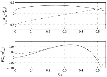
Figure 1: Upper panel: $\left\langle f_{j}\right\rangle$ (solid) and $\left\langle f_{\Omega}\right\rangle$ (dashed) from Eqs. (19). Lower panel: $F$ from Eq. (23) (solid line) and its quadratic approximation Eq. (23) (dashed line)

Eqs. (16),(19) and (12) form a closed set of equations for the slowly varying $j_{z},C_{K}$ and $\Omega_{e}$. An example of a numerical integration of these equations, compared with the results of a direct integration of the secular equations (6) is shown in figure 2 for $\epsilon_{\text{Oct}}=0.01$. As can be seen the approximate equations describe the long term evolution to a good approximation.

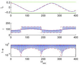
Figure 2: Results of numerical integrations for initial conditions $\epsilon_{\text{Oct}}=0.01,~{}\omega_{0}=0,~{}\Omega_{0}=\pi,i_{0}=80^{o},e_{0}=0.1$. The blue solid lines are the result of the direct integration of Eqs. (6) while the red dashed lines are the results of integrating Eqs. (16),(19) and (12) and using the pure Kozai relations to extract $e_{\min},e_{\max}$ and $i_{\min},i_{\max}$. The two green horizontal lines in the top panel represent $\pm j_{\max}$, given by Eq.(15)

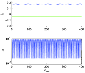
Figure 3: Results of numerical integrations for initial conditions identical to the parameters in figure 2 except for $\omega_{0}=\pi/2$ replacing $\omega_{0}=0$, for which the Kozai cycles are rotating. The blue solid line is the result of the direct integration of Eqs. (6). The two green horizontal lines represent $\pm j_{\max}$, given by Eq.(15)

These equations break down if $\left|j_{z}\right|$ crosses the threshold Eq. (15), in which case $\Omega_{e}$ receives kicks, $\dot{j}_{z}$ changes sign, $j_{z}$ moves to the rotation region after a few secular time scales and the averaged equations become valid again. An example of such behavior is seen in fig 4. In this example, the effective equations Eqs. (16),(19) and (12) were integrated only in the intervals were $C_{K}>0$ (dashed lines).

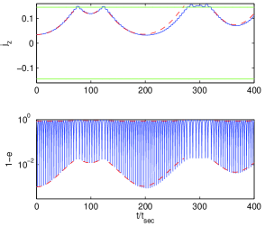
Figure 4: Results of numerical integrations for initial conditions $\epsilon_{\text{Oct}}=0.01,~{}\omega_{0}=0,~{}\Omega_{0}=0,i_{0}=88^{o},e_{0}=0.1$. The blue solid line is the result of the direct integration of Eqs. (6) while the red dashed line is the result of integrating Eqs. (16),(19) and (12) in the regions were $C_{K}>0$ (corresponding to $|j_{z}|<j_{\max}$, the region within the two green horizontal lines given by Eq.(15))

.

Analytic solution

Eqs. (16),(19) and (12) are integrable. These equations have a constant of motion of the form

$$C=F(C_{K})-\epsilon_{\rm oct}\cos(\Omega_{e}).$$ (22)

Indeed, using (16) and (12) we find, $\dot{C}=\epsilon_{\rm oct}j_{z}\sin\Omega_{e}(F^{\prime}\left\langle f_{j}\right\rangle-\left\langle f_{\Omega}\right\rangle),$ and by setting

$$F(C_{K}) =\int_{0}^{C_{K}}\frac{\left\langle f_{\Omega}\right\rangle(c)}{\left\langle f_{j}\right\rangle(c)}dc$$ (23)

$$=32\frac{\sqrt{3}}{\pi}\int_{\frac{3-3C_{K}}{3+2C_{K}}}^{1}\frac{K(x)-2E(x)}{(41x-21)\sqrt{2x+3}}dx$$ (24)

we obtain $\dot{C}=0$. The numerical value of $F(e_{\min}^{2})$ as a function of $e_{\min}$ is shown in the bottom panel of figure 1 and tabulated in the attached file e2F.txt.

Note that $F$ diverges at $e_{\min,\inf}=(4/11)^{0.5}$ where $\left\langle f_{j}\right\rangle=0$. For $e_{\min}>e_{\min,\inf}$, the integration limits in Eq. (23) should be chosen differently. Here we focus on $e_{\min}<e_{\min,\inf}$. $F$ has a maximum $F_{\max}\approx 0.0475$ at $e_{\min,m}^{2}=(3-3x_{m})/(3+2x_{m})\approx 0.112$ where $x_{m}$ is the solution to the equation $K(x_{m})=2E(x_{m})$ (at which $\left\langle f_{\Omega}\right\rangle=0$). Near maximum, $F$ can be well approximated by a quadratic expression,

$$F(e_{\min}^{2})\approx F_{\max}-2.67(e_{\min}^{2}-e_{\min,m}^{2})^{2},$$ (25)

(shown as dashed line in the bottom panel of figure 1).

This constant of motion holds most of the information about the system.

Flip criterion

We next use the constant of motion Eq. (22) to derive a criterion of the initial conditions which is necessary in order that $j_{z}$ ”flips” i.e. changes sign (implying $i$ goes above $90^{o}$ and the orbit becomes retrograde relative to the perturber).

During a flip, $j_{z}=0$ and Eq. (12) implies that $C_{K}=C_{K,0}+0.5j_{z,0}^{2}$. Given the constant of motion Eq. (22), and that the term $\epsilon_{\text{Oct}}\cos\Omega_{e}$ can change by at most $2\epsilon_{\text{Oct}}$, a required condition for a flip is that $\epsilon_{\text{Oct}}>\epsilon_{\text{Oct},c}$ where

$$\epsilon_{\text{Oct},c}=\frac{1}{2}\max\left(\left|\Delta F(x)\right|\right)$$ (26)

where $x$ is in the range $C_{K,0}<x<C_{K,0}+0.5j_{z,0}^{2}$ and $\Delta F(x)=F(x)-F(C_{K,0})$. Given that $F$ has one maximum at $C_{K,m}=e_{\min,m}^{2}$, the condition can be separated as follows: If $C_{K,0}+0.5j_{z,0}^{2}<C_{K,m}$, or $C_{K,0}>C_{K,m}$, so that the initial and final $C_{K}$ are on the same side of the location of $C_{K,m}$, $\epsilon_{\text{Oct},c}=\left|F(C_{K,0}+0.5j_{z,0}^{2})-F(C_{K,0})\right|$. Otherwise, if the initial and final $C_{K}$ are on different sides of $C_{K,m}$, the value of $\epsilon_{\text{Oct}}$ is the larger of $\epsilon_{\text{Oct},c}=\left|F(C_{K,0}+0.5j_{z,0}^{2})-F(C_{K,0})\right|$ and $\epsilon_{\text{Oct},c}=F_{\max}-F(C_{K,0})$. The presence of $F_{\max}$ thus creates a discontinuity in the flip condition (see figures 5 and 6). For cases where initially $e_{0}\ll 1$ implying that $C_{K}\ll 1$ and $j_{z,0}=\cos i_{0}$, and for $j_{z,0}^{2}<2e_{\min,m}^{2}$ ($i_{0}>61.7^{o}$), Eq. (26) reduces to

$$\epsilon_{Oct,c}=\frac{1}{2}F(\frac{1}{2}\cos^{2}i_{0}).$$ (27)

This analytic theoretical line is shown in solid blue in the upper panel of figure 5. For comparison, the results of numerical integrations of Eqs. (6) over $10/\epsilon_{\text{Oct}}$ secular times for corresponding $\epsilon_{\text{Oct}},~{}i_{0}$ with $\omega_{0}=0$, $e_{0}=0.001$ and $\Omega_{0}$ scanned over $0-2\pi$ are shown in filled red (flipped) and empty blue (no flip) circles. The analytical curve describes the flip condition to better than 10% for $i_{0}\gtrsim 80$ deg, better than 20% for $i_{0}>70$ deg, and to a factor less than $2$ for $i>50$ deg. The deviation at low inclinations is not surprising, given that our formalism assumes $j_{z}^{2}\ll 1$. It is encouraging that the overall behaviour is captured quite well for $j_{z}$ up to 0.5.

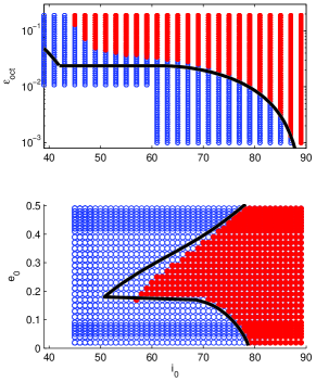
Figure 5: Upper Panel: The solid black line is the threshold, Eq. (26), for a flip given that we start with $e_{0}\sim 0$ (this reduces to (27) for $i>61.7^{o}$). Red circles are results of numerical integrations ($e_{0}=0.001$, $\omega_{0}=0$, $\Omega_{0}=0-2\pi$) that had a flip while blue circles are simulations that didn’t. Lower Panel: The solid black line is the flip threshold, Eq. (26), for $\epsilon_{\text{Oct}}=0.01$. Red circles are results of numerical integrations ($\omega_{0}=0$, $\Omega_{0}=0-2\pi$) that had a flip while blue circles are simulations that didn’t.

The curve representing Eq. (26) for $\epsilon_{\text{Oct},c}=0.01$ on the $e_{\min,0},i_{0}$ plane is shown in the lower panel of figure 5 (solid black). For comparison, the results of numerical integrations for corresponding $e_{\min,0},i_{0}$ are shown in filled red (flipped) and empty blue (no flip) circles.

The result of Eq. (26) for different values of $e_{\min}$ is shown in figure 6.

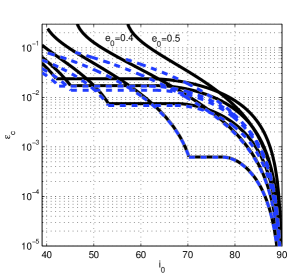
Figure 6: The theoretical threshold Eq. (26), for a flip for different initial $e_{\min}$ ($e_{0}$ at $\omega=0$). The black solid lines show the result of Eqs. (26) and (23), for $e_{\min}=0.001,0.1,0.2,0.3,0.4,0.5$ (lines in the top left corner are ordered low $\epsilon_{\text{Oct},c},i_{0}$ to high $\epsilon_{\text{Oct},c},i_{0}$ for growing $e_{\min}$). The dashed blue curves are the corresponding results of Eq.(26), with the approximate expression for $F$, Eq. (25).

Maximal $e$ and General Relativity (GR) precession

A rough estimate of the typical maximal eccentricity expected during an episode when $j_{z}$ crosses zero, can be obtained as follows and was confirmed in several numerical test runs with various parameters. The assumption is that at maximal $e$ we have $j\sim|j_{z}|$. Since the maximal $e$ will be obtained in some arbitrary phase in the Kozai cycle during which $j_{z}$ crosses zero, we expect $1-e_{\max}^{2}=j^{2}\sim j_{z}^{2}\sim(0.5\dot{j}_{z}\tau_{\rm Koz})^{2}\sim\epsilon_{\text{Oct}}^{2}$ (where we assumed that $\Omega_{e}$ is not tuned to $0$ or $\pi$ so that ($\sin^{2}\Omega_{e}\sim 1$). In fact we expect a roughly uniform distribution of $j_{z}$ or $[1-\max(e)]^{1/2}$ around this range. General relativistic corrections cause the pericenter to rotate and can be incorporated into the equations of motion by adding a term $\phi_{\rm GR}=\epsilon_{\rm GR}/j$ to the total normalized averaged potential $\phi$Fabrycky & Tremaine (2007), where $\epsilon_{\rm GR}=3GM^{2}/M_{\text{per}}a^{-4}a_{\text{per}}^{3}$. This effect suppresses the maximal eccentricity in the Kozai-Lidov cycles when $\epsilon_{\rm GR}/j\sim 1$ Fabrycky & Tremaine (2007); using the estimate above for $e_{\max}$, GR becomes significant once $\epsilon_{\rm GR}\sim\epsilon_{\text{Oct}}$. If this occurs, e can change its direction considerably during one Kozai-Lidov cycle, $\Omega_{e}$ may change by $\sim\pi$, causing $\dot{j}_{z}$ to change sign avoiding a flip. We verified this rough criterion for suppression of flips numerically.

Kozai-migrated Hot Jupiters by distant, stellar mass perturbers

Recently, numerical simulations by (Naoz et al., 2011) showed that Jupiter-mass planets, perturbed by comparable planetary or brown dwarf mass perturbers, undergo slowly modulated Kozai-Lidov cycles, and exhibit striking features, including extremely high eccentricities and the generation of retrograde orbits with respect to the perturber. Those authors attributed the slow modulation of the Kozai-Lidov cycles to the relative proximity and comparable mass of the perturber to the perturbed planet, and the high eccentricities to chaotic evolution; they suggested that these effects would not occur in the case of distant stellar mass perturbers.

Our analytical and numerical analysis shows that these effects have a simpler explanation: the octupole perturbation alone modulates the Kozai-Lidov cycles, and it does so non-chaotically to excite the extremely high eccentricities and the retrograde inclinations. This effect occurs already in the test particle approximation in which the mass of the perturber is much bigger than that of the planet, and will thus be important for stellar mass perturbers. In fact, similar evolution occurs in other cases where there are small deviations from axisymmetry Katz & Dong (2011).

Consequently the distribution of orbital parameters of Kozai-migrated hot Jupiters due to a stellar perturber may be significantly affected by the dynamics of the octupole perturbations described in this Letter.

Consider for example, the system parameters studied numerically in Fabrycky & Tremaine (2007), $a=5\rm AU$, $a_{\text{per}}=500\rm AU$, $M=M_{\text{per}}=M_{\odot}\sim 1000M_{J}$, where the contribution of the octupole term was neglected. The perturber eccentricity in this study was set to 0 for convenience (which implies zero octupole contribution), but in reality is expected to have a wide distribution of values. Such a system has an octupole coefficient, ${\epsilon_{\text{Oct}}=aa_{\text{per}}^{-1}e_{\text{per}}/(1-e_{\text{per}}^{2})}\approx 0.01$, secular time scale of ${t_{\rm sec}\propto M^{1/2}M_{\text{per}}^{-1}a^{-2}a_{\text{per}}^{3}}=1.8\times 10^{6}\mbox{ yr}$, and GR precession coefficient of ${\epsilon_{\rm GR}\propto M^{2}M_{\text{per}}^{-1}a^{-4}a_{\text{per}}^{3}}=4.7\times 10^{-5}$.

We performed a few test runs with these parameters (including GR precession but not tidal dissipation) and found that extremely high eccentricities $1-e_{\max}\sim 10^{-4}$ can be reached for inclinations $i>80^{\circ}$ (in reality, $e_{\max}$ would be limited by other physical effects). For the runs we made, a flip was suppressed due to the GR precession, but for equally likely parameters with slightly closer perturbers, $a_{\rm per}\lesssim 300\rm AU$ the effect of GR precession becomes negligible and flips are also attainable in accordance with the criterion Eq. (26).

A numerical investigation of this problem is published simultaneously by a different group in Lithwick & Naoz (2011).

We thank Scott Tremaine, Jihad Touma, Yoram Lithwick, Fred Rasio, Smadar Naoz and Will Farr for useful discussions. B.K. is supported by NASA through Einstein Postdoctoral Fellowship awarded by the Chandra X-ray Center, which is operated by the Smithsonian Astrophysical Observatory for NASA under contract NAS8-03060. Work by SD was performed under contract with the California Institute of Technology (Caltech) funded by NASA through the Sagan Fellowship Program.

References

- Mayor & Queloz (1995) Mayor, M., & Queloz, D. 1995, Nature (London), 378, 355
- Lidov (1962) Lidov, M. L. 1962, Planetary and Space Science, 9, 719
- Kozai (1962) Kozai, Y. 1962, Astron. J., 67, 591
- Heisler & Tremaine (1986) Heisler, J., & Tremaine, S. 1986, Icarus, 65, 13
- Blaes et al. (2002) Blaes, O., Lee, M. H., & Socrates, A. 2002, Astrophys. J., 578, 775
- Fabrycky & Tremaine (2007) Fabrycky, D., & Tremaine, S. 2007, Astrophys. J., 669, 1298
- Perets & Naoz (2009) Perets, H. B., & Naoz, S. 2009, Astrophys. J. Lett., 699, L17
- Thompson (2010) Thompson, T. A. 2010, arXiv:1011.4322
- Tremaine et al. (2009) Tremaine, S., Touma, J., & Namouni, F. 2009, Astron. J., 137, 3706
- Ford et al. (2000) Ford, E. B., Kozinsky, B., & Rasio, F. A. 2000, Astrophys. J. , 535, 385
- Naoz et al. (2011) Naoz, S., Farr, W. M., Lithwick, Y., Rasio, F. A., & Teyssandier, J. 2011, Nature (London), 473, 187
- Milankovich (1939) Milankovich, M. 1939, Bull. Serb. Acad. Math. Nat. A, 6, 1
- Allan & Ward (1963) Allan, R. R., & Ward, G. N. 1963, Proceedings of the Cambridge Philosophical Society, 59, 669
- Katz & Dong (2011) Katz, B., & Dong, S. 2011, arXiv:1105.3953
- Lithwick & Naoz (2011) Lithwick Y., & Naoz S. 2011