Tunable Supercurrent at the Charge Neutrality Point via Strained Graphene Junctions

Abstract

We theoretically calculate the charge-supercurrent through a ballistic graphene junction where superconductivity is induced via the proximity-effect. Both monolayer and bilayer graphene are considered, including the possibility of strain in the systems. We demonstrate that the supercurrent at the charge neutrality point can be tuned efficiently by means of mechanical strain. Remarkably, the supercurrent is enhanced or suppressed relative to the non-strained case depending on the direction of this strain. We also calculate the Fano factor in the normal-state of the system and show how its behavior varies depending on the direction of strain.

I Introduction

Since the discovery of graphene cite:novoselov1 , many interesting phenomena have been predicted in the context of quantum transport in this material cite:beenakker1 ; cite:Titov1 ; cite:Tworzydlo ; cite:Snyman ; cite:Ossipov . It has been demonstrated in several theoretical and experimental works that the conductivity of graphene monolayer junctions at zero doping level (the charge neutrality point aka Dirac point) displays a minimum value in the short junction regime cite:novoselov1 ; cite:zhang ; cite:Tworzydlo ; cite:Titov1 ; cite:Akhmerov . The physical reason for the minimum conductivity in this regime is the existence of evanescent modes that can transport current over a finite length $L$ of the system. A unique aspect of graphene is that these evanescent modes are predicted to generate pseudo-diffusive characteristics of the quantum transport properties even in ballistic graphene samples cite:Tworzydlo .

Bilayer graphene is a basic carbon structure and has attracted considerable attention recently. This system consists involved two coupled graphene layers with prominent characteristics such as pseudospin and variable chirality cite:choi2 . The chirality of the massless Dirac fermions in monolayer graphene is locked to the momentum direction and consequently lies in the plane of the sheet. In bilayer graphene, however, massive Dirac fermions with perpendicular chirality to the sheet plane may occur. Bilayer graphene features a band-structure similar to a semiconductor with parabolic bands with a tunable charge excitation gap cite:choi1 ; zhang1 ; ostinga ; cite:castro ; kuzmenko ; li ; maik . A gapless graphene bilayer is more stable compared to its gapped equivalence and thus occurs naturally. Bilayer graphene has also shown anomalous phenomena such as half-integer quantum Hall effect, minimum conductivity at zero energy and $2\pi$ Berry phase.

Very recently, the response of graphene to strain has been intensively examined. Several unusual effects have been unveiled, including the generation of very high pseudo-magnetic fields of order 300 T cite:levy_science_10 . An interesting question in this context relates to if strain imposed on graphene, whether it be mechanical or thermal in origin, can be used to control its transport properties cite:peres_rmp_10 . This issue is also motivated by the well-known fact that strain imposed on silicon-based devices can enhance their functionality. A mechanical deformation of a graphene sheet will invariably generate scattering centers which effectively influences the hopping amplitude, and thus suggests that the transport of Dirac fermions should respond to the presence of strain. It is known that strain may change the physical properties of nanotubes drastically yang2 ; tombler ; minot ; cite:choi1 ; cite:choi2 . The strain can be induced in graphene via several routes, including mechanically mohi ; ferralis ; kim ; huang ; teague .

Based on this idea, we address in this paper a novel class of the Josephson graphene junctions with the capability to sustain tuneable charge-transport at the Dirac point by means of mechanically induced strain. To demonstrate this, we first solve the Bogoliubov de-Gennes equations both for a strained monolayer and bilayer graphene-based superconductor$\mid$normal$\mid$superconductor (S$\mid$N$\mid$S) junction with heavily doped S regions, as is experimentally relevant. We then derive explicit analytical expressions for the Andreev-levels and use these to obtain the phase-dependent supercurrent $I(\phi)$ in the short-junction regime cite:beenakker2 . Both the critical current $I_{c}$ and the $I_{c}R_{N}$ product is investigated for a range of doping levels in the N region, including the charge neutrality point. Above, $R_{N}$ is the normal state resistance. Finally, we calculate the Fano factor $F$ in the normal (non-superconducting) state and show how this is influenced by the presence of mechanical strain in the system.

To describe strained graphene, we adopt the model used in Ref.cite:Pereira, for monolayer graphene and also consider a similar model for strained graphene bilayer junctions. Our findings show that for a zig-zag ($Z$)-strain (see Fig.1) the transmission probability of evanescent modes near the charge neutrality point is suppressed, which influences both the conductivity $\sigma$ and the supercurrent. However, when the strain is applied along the armchair ($A$) direction instead, the transmission probability is enhanced and correspondingly influences charge-transport in the system. These results point towards new perspectives within tunable quantum transport by means of induced strain in a graphene mono- or bilayer. This finding might also be of relevance in the field of spintronics (valleytronics), since the strain also affects the pseudo-spin of the chiral fermions in graphene cite:choi1 ; cite:choi2 .

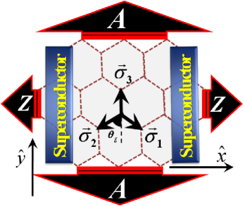
Figure 1: The schematical setup of a strained graphene Josephson junction. The two superconducting electrode interfaces are located at $x=0,L$. There is also a controllable gate voltage for tuning the concentration of carriers (not shown). $Z$ and $A$ stand for zig-zag and armchair strains while $\sigma_{i}$ represent displacement vectors of the three nearest neighbors C atoms in the strained graphene. $\theta_{g}$ is the strained angle between C-C junctions which can be either larger or smaller than the non-strained value $60^{\circ}$.

The paper is organized as follows: In Sec. II, we present our theoretical approach and derive a general expression for the normal-state transition probabilities describing both strained monolayer and bilayer junctions. In this section, we also discuss an experimental setup for detecting our predictions. In Sec. III, the Andreev subgap bound state energies for both strained monolayer and bilayer S$\mid$N$\mid$S Josephson junctions are obtained and the subsequent results are discussed. We finally conclude our findings in Sec. IV.

II Theoretical Approach and Model

The two graphene systems considered in this paper (monolayer and bilayer) are modelled via the following Hamiltonians cite:beenakker3 ; cite:mccann1 ; cite:nilsson ; cite:Snyman ; cite:castro ($\mathcal{S}$ and $\mathcal{B}$ stand for single- and bilayer graphene under strain, respectively):

$$\mathcal{H}_{\pm}^{\mathcal{S}}=v_{x}p_{x}\sigma_{x}\pm v_{y}p_{y}\sigma_{y}+U$$ (1)

$$\mathcal{H}^{\mathcal{B}}=\left(\begin{array}[]{cccc}U&\pi&0&0\\ \pi^{{\dagger}}&U&t_{\bot}&0\\ 0&t_{\bot}&U&\pi^{{\dagger}}\\ 0&0&\pi&U\\ \end{array}\right)$$ (2)

where $\pi$$=$$v_{x}p_{x}$$+$$iv_{y}p_{y}$ and $v_{x,y}$ are the Fermion velocities in the $\hat{x},\hat{y}$-directions while $\sigma_{x,y}$ are Pauli matrices. Here, $U$ represents an external gate potential. The $\pm$ signs refer to the $\mathbf{K}$ and $\mathbf{K^{\prime}}$ valleys of monolayer graphene. We here consider an $A_{2}B_{1}$ stack for the bilayer graphene sheet and use a tight-binding model in which the massive chiral Dirac frmions are governed by Eq. (2). The resulting Hamiltonian becomes similar to a gapless semiconductor Hamiltonian with parabolic electron and hole bands touching when $t$$\rightarrow$$\infty$. In order to model applied strain to the system, we adopt the model of Ref. cite:Pereira, and expand the tight-binding model band structure with arbitrary hopping energies $t_{1,2,3}$ i.e. $\epsilon=\pm\mid\sum_{i=1}^{3}t_{i}e^{-i\overrightarrow{k}\cdot\overrightarrow{\sigma_{i}}}\mid$ around the Dirac point, $\mathbf{K}_{D}=(\cos^{-1}(-1/2\eta)/\sqrt{3}a_{x},0)$ cite:choi1 ; cite:soodchomshom . As shown in Fig. 1, $\overrightarrow{\sigma_{i}}$ are displacement vectors between three nearest C atoms (see Ref. cite:paper_sigma_i, ). We assume $t_{1,2}=t_{\vdash}$ and $t_{3}=t$ in our calculations and set $\eta$ as the ratio $t_{\vdash}/t$. This assumption generates asymmetric Fermion velocities along the different directions. These velocities are given by $v_{x}=2t_{\vdash}a_{x}\sin(\cos^{-1}(-1/2\eta))/\hbar$ and $v_{y}=3ta_{y}/2\hbar$ cite:choi1 ; cite:choi2 ; cite:soodchomshom . The next-nearest neighbor hopping (n.n.n.) in graphene can cause the Dirac cone to be tilted, this effect vanishes under the influence of strain of order $\sim$ 20% cite:choi1 . In this regime, the generalized Weyl-Hamiltonian used here gives very good agreement with ab initio calculations. We note that it is also possible to model strained graphene by including a fictious gauge-potential $\mathbf{A}$ peres_rmp_10 . Motivated by the results of Ref. cite:Snyman, for bilayer graphene junctions, we here adopt the same model as the strained monolayer for the strained bilayer whereas the interlayer hopping $t_{\bot}$ is left intact as the strain is applied in-plane. We emphasize that in this paper the same model for clean doped bilayer graphene region is adopted as Ref. cite:Snyman, and consequently the trigonal warping effects may be neglected.

In both cases, we consider an S$\mid$N$\mid$S junction with $s$-wave superconducting electrodes. Previous works have been considered the Josephson effect in non-strained monolayer graphene cite:Titov1 ; cite:cuevas ; blackschaffer_prb_08 . We assume that the Fermi wavelengths satisfy $\lambda_{N}\gg\lambda_{S}$, corresponding to heavily doped S regions. In this regime, we may ignore interface details and consider the following $x$-dependent superconducting order parameter as depicted in Fig.1 (see Ref. cite:halterman, );

$$\Delta(x)=\left\{\begin{array}[]{cc}\Delta(T)e^{i\phi_{l}}&x<0\\ 0&0<x<L\\ \Delta(T)e^{i\phi_{r}}&x>L\\ \end{array}\right..$$ (6)

By substituting the Hamiltonians Eq.(1) and Eq.(2) into the Bogoliubov-de Gennes equation

$$\left(\begin{array}[]{cc}\mathcal{H}-\mu&\Delta\\ \Delta^{*}&\mu-\mathcal{H}\end{array}\right)$$ (7)

where $\mu$ is the chemical potential, we find the following energy-momentum dispersion relations:

$$\left\{\begin{array}[]{c}\varepsilon^{\mathcal{B}}=\left[\Delta^{2}+\left\{\mu\pm\frac{t_{\bot}}{2}\pm\frac{1}{2}\sqrt{t_{\bot}^{2}+4\hbar^{2}|k|^{2}\nu^{2}}\right\}^{2}\right]^{\frac{1}{2}}\\ \varepsilon^{\mathcal{S}}=\left[\Delta^{2}+\left\{\mu\pm\hbar|k|\nu\right\}^{2}\right]^{\frac{1}{2}}\\ \nu^{2}=v_{x}^{2}\cos^{2}\theta+v_{y}^{2}\sin^{2}\theta\end{array}\right.$$ (8)

Above, $\theta$ is the angle of incidence of the particles. The eigenfunctions of Eq.(7) for the strained monolayer and bilayer systems within the normal region are found to be:

$${}^{\mathcal{S}}\left\{\begin{array}[]{c}\Psi_{e^{\pm}}^{N}=(\pm a_{e^{\pm}}^{N},1,\mathbf{0}^{\mathcal{S}})^{T}e^{\pm i\hbar k_{e}^{N}x}\\ \Psi_{h^{\pm}}^{N}=(\mathbf{0}^{\mathcal{S}},\mp a_{h^{\pm}}^{N},1)^{T}e^{\pm i\hbar k_{h}^{N}x}\end{array}\right.$$ (11)

$${}^{\mathcal{B}}\left\{\begin{array}[]{c}\Psi_{e^{\pm}}^{N}=(-1,\mp a_{e^{\pm}}^{N},\pm a_{e^{\pm}}^{N},1,\mathbf{0}^{\mathcal{B}})^{T}e^{\pm i\hbar k_{e}^{N}x}\\ \Psi_{h^{\pm}}^{N}=(\mathbf{0}^{\mathcal{B}},-1,\mp a_{h^{\pm}}^{N},\pm a_{h^{\pm}}^{N},1)^{T}e^{\pm i\hbar k_{h}^{N}x}\end{array}\right.$$ (14)

where $\mathbf{0}^{\mathcal{S}}$ and $\mathbf{0}^{\mathcal{B}}$ represent $1\times 4$- and $1\times 2$-spinors with only zeroes as entries, while $e$ and $h$ stand for electron and hole particles. The $\pm$ sign refers to right and left going particles. The coefficients $a_{e^{\pm}}^{N}$ and $a_{h^{\pm}}^{N}$ are defined as follows:

$$^{\mathcal{S}}\left\{\begin{array}[]{c}a_{e^{\pm}}^{N}=\frac{\mu+\varepsilon}{\hbar k_{e}^{N}(v_{x}\cos\theta\pm iv_{y}\sin\theta)}\\ a_{h^{\pm}}^{N}=\frac{\mu-\varepsilon}{\hbar k_{h}^{N}(v_{x}\cos\theta_{A}\pm iv_{y}\sin\theta_{A})}\\ \hbar k_{e(h)}^{N}=\frac{\mu(\pm)\varepsilon}{\nu}\end{array}\right.$$ (18)

$$^{\mathcal{B}}\left\{\begin{array}[]{c}a_{e^{\pm}}^{N}=\frac{\mu+\varepsilon}{\hbar k_{e}^{N}(v_{x}\cos\theta\pm iv_{y}\sin\theta)}\\ a_{h^{\pm}}^{N}=\frac{\mu-\varepsilon}{\hbar k_{h}^{N}(v_{x}\cos\theta_{A}\pm iv_{y}\sin\theta_{A})}\\ \hbar k_{e(h)}^{N}=\sqrt{\frac{t(\mu(\pm)\varepsilon)}{\nu^{2}}}\end{array}\right.$$ (22)

For the bilayer system, we consider the hopping value between the graphene layers to be smaller than the doping level of superconducting regions, still much larger than the superconducting gap that is $\mu^{s}\gg t\gg\varepsilon_{F},\varepsilon$ cite:ludwig . The former assumption assures ignoring the contact details in the S$\mid$N interfaces while the latter not only helps to simplify theoretical approach but also warranties realistic approximations in our analytical calculations. Within the normal region in which superconducting order parameter $\Delta$$=$$0$, the Eq. (7) leads to uncoupled equations. In this paper, we focus on the low-energy regime. One then finds the following parabolic dispersion relation for electrons and holes in the normal bilayer region:

$$\varepsilon^{\mathfrak{B}}=\left|\varepsilon_{F}\pm\left(\frac{(\hbar v|k|)^{2}}{t}\right)\right|.$$ (23)

Due to translational symmetry in the transverse direction, $k_{y}$ and $\varepsilon$ are both conserved upon reflections at the interfaces located at $x=0,L$. Accordingly, the dispersion relations and the following equation assure both energy and momentum conservation of particles in the $y$-direction upon Andreev electron-hole conversion,

$$k_{e}^{N}\sin\theta=k_{h}^{N}\sin\theta_{A}=q_{n}=2n\pi/W$$

$$k_{e}^{N}\sin\theta=k_{e,h}^{S}\sin\theta_{e,h}^{S}=q_{n}=2n\pi/W.$$ (24)

The total spinors in the three regions thus read:

$$\Psi^{N} = e^{i\hbar q_{n}y}(a_{1}\Psi_{e^{+}}^{N}+a_{2}\Psi_{e^{-}}^{N}+b_{1}\Psi_{h^{+}}^{N}+b_{2}\Psi_{h^{-}}^{N})$$

$$\Psi_{r}^{S} = e^{i\hbar q_{n}y}(t_{e}^{r}\Psi_{e^{+}}^{S}(\phi_{r})+t_{h}^{r}\Psi_{h^{+}}^{S}(\phi_{r}))$$ (25)

$$\Psi_{l}^{S} = e^{i\hbar q_{n}y}(t_{e}^{l}\Psi_{e^{-}}^{S}(\phi_{l})+t_{h}^{l}\Psi_{h^{-}}^{S}(\phi_{l})).$$

In superconductor spinors, we define the following relation for superconducting coherent factors (see Appendix):

$$\beta=\left\{\begin{array}[]{cc}\cos^{-1}(\varepsilon/\Delta)&\varepsilon<\Delta\\ -i\cosh^{-1}(\varepsilon/\Delta)&\varepsilon>\Delta\\ \end{array}\right.$$ (26)

the definition helps to simplifying our notation. The spinors in the superconducting regions carry $S$ superscript, whereas $r$ and $l$ stand for right and left superconducting regions. The superconducting phases in each region are assumed to be $\phi_{r}$ and $\phi_{l}$, while $t_{h}$ and $t_{e}$ are the scattering amplitudes of hole- and electron-like quasiparticles. Matching the total wavefunctions at each of the interfaces, i.e.

$$\Psi_{l}^{S}\mid_{x=0}=\Psi^{N}\mid_{x=0}\;\;\;\text{and}\;\;\;\Psi_{r}^{S}\mid_{x=L}=\Psi^{N}\mid_{x=L}$$ (27)

leads a quantization relation between superconducting phase difference $\phi=\phi_{r}-\phi_{l}$ and the quasiparticle excitation energy $\varepsilon$. The boundary conditions lead to a 8$\times$8 matrix M for transmission and reflection coefficients which is presented in the Appendix for monolayer case cite:linder1 . $det(\emph{M})=0$ generates a non-trivial relation between $\varepsilon$ and $\phi$ as follow;

$$\digamma_{1}+\digamma_{2}\sin 2\beta+\digamma_{3}\cos 2\beta=0,$$ (28)

$$\digamma_{1}=-(a_{e^{-}}^{N}+a_{e^{+}}^{N})(a_{h^{-}}^{N}+a_{h^{+}}^{N})\cos\phi$$

$$+\sin(k_{h}^{N}L)\sin(k_{e}^{N}L)((-a_{e^{+}}^{N}a_{h^{-}}^{N}-a_{h^{+}}^{N}a_{h^{-}}^{N}+a_{e^{+}}^{N}a_{h^{+}}^{N}$$

$$-a_{e^{-}}^{N}(-a_{h^{-}}^{N}a_{h^{+}}^{N}a_{e^{+}}^{N}+a_{e^{+}}^{N}-a_{h^{-}}^{N}+a_{h^{+}}^{N})+1)$$

$$\digamma_{2}=\sin(k_{e}^{N}L)(a_{e^{-}}^{N}a_{e^{+}}^{N}+1)(a_{h^{-}}^{N}+a_{h^{+}}^{N})\cos(k_{h}^{N}L)$$

$$+(a_{e^{-}}^{N}+a_{e^{+}}^{N})\cos(k_{e}^{N}L)(a_{h^{-}}^{N}a_{h^{+}}^{N}+1)\sin(k_{h}^{N}L)$$

$$\digamma_{3}=-\sin(k_{h}^{N}L)\sin(k_{e}^{N}L)(a_{e^{-}}^{N}a_{e^{+}}^{N}+1)(a_{h^{-}}^{N}a_{h^{+}}^{N}+1)$$

$$+(a_{e^{-}}^{N}+a_{e^{+}}^{N})\cos(k_{e}^{N}L)(a_{h^{-}}^{N}+a_{h^{+}}^{N})\cos(k_{h}^{N}L)$$

We here employ the most relevant experimentally approximation i.e. the ”short-junction” regime in which $\Delta L/\hbar v\ll 1$. Within this regime, $\digamma_{1}$, $\digamma_{2}$ and $\digamma_{3}$ are reduced to the following expressions;

$$\digamma_{1}=-(a_{e^{-}}^{N}+a_{e^{+}}^{N})^{2}\cos\phi+\sin^{2}(kL)$$

$$\times((a_{e^{+}}^{N})^{2}+a_{e^{-}}^{N}(-(a_{e^{+}}^{N})^{2}a_{e^{-}}^{N}+a_{e^{-}}^{N})-1)$$

$$\digamma_{2}=0$$ (29)

$$\digamma_{3}=\sin^{2}(kL)(a_{e^{-}}^{N}a_{e^{+}}^{N}+1)^{2}+(a_{e^{-}}^{N}+a_{e^{+}}^{N})^{2}\cos^{2}(kL).$$

In this case, using the definition of $\beta$ and Eq.(28) the single Andreev bound state is obtained vs $\digamma_{1}$ and $\digamma_{3}$

$$\frac{\varepsilon}{\Delta}=\sqrt{\frac{1}{2}\left(1-\frac{\digamma_{1}}{\digamma_{3}}\right)}\;\;\text{and then}$$

$$\varepsilon_{n}(\phi)=\Delta\sqrt{1-\tau_{n}\sin^{2}\phi/2}$$

in which $\tau_{n}$ is transmission probability for the normal graphene region between two strongly doped electrodes (either superconductor or normal). After some calculations we reach at an expression for $\tau_{n}$ valid for both strained monolayer and bilayer systems i.e.

$$\tau_{n}=\frac{(a_{e^{+}}^{N}+a_{e^{-}}^{N})^{2}}{(a_{e^{+}}^{N}+a_{e^{-}}^{N})^{2}\cos^{2}(k_{n}L)+(a_{e^{+}}^{N}a_{e^{-}}^{N}+1)^{2}\sin^{2}(k_{n}L)}.$$ (30)

We utilize the general $\tau_{n}$ for investigating the transport properties of the strained monolayer and bilayer junctions in the next section.

The contribution of the Andreev bound-state spectrum to the supercurrent is given by cite:Titov1 ; cite:beenakker2 :

$$I(\phi)=\frac{e\Delta^{2}}{\hbar}\sum_{n=0}^{\infty}\tau_{n}\sin\phi/\varepsilon_{n}(\phi).$$ (31)

For a wide graphene junction, $W$$\gg$$L$, the boundary conditions (zig-zag and armchair) at the edges $y$$=$$W/2$ and $-W/2$ are irrelevant and we here assume smooth boundaries for the two edges. In this regime, we may replace the summation over quantized modes with an integration: $\sum_{n}$$\rightarrow$$W/\pi$$\int$$dq_{n}$. Now we proceed in the following sections to study the supercurrent using Eqs. (18), (22) and (31) for monolayer and bilayer Josephson junctions in particular at the charge neutrality point i.e. $\mu\rightarrow 0$.

III Supercurrent, Fano Factor and Andreev Bound States in Strained Graphene Monolayer/Bilayer S$\mid$N$\mid$S Junction

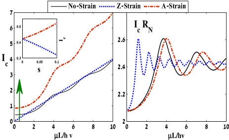
Figure 2: The critical current $I_{c}$ (left panel) and its product with the normal-state resistance $I_{c}R_{N}$ (right panel) as a function of $\mu L/\hbar v$ for a monolayer system. The solid line pertains to a non-strained junction. For $Z$-tension $t_{\vdash}=0.56t_{0},\;t=1.1t_{0}$ while for $A$-strain $t_{\vdash}=0.95t_{0},\;t=0.5t_{0}$. The arrow indicates how the Josephson current may be enhanced by means of the applied direction of tension to the system. The inset panel shows critical supercurrent as a function of strain.

By inserting Eq.(18) for the monolayer system into Eq.(30), the following expressions are obtained:

$$\tau_{n}^{\mathcal{S}}=\frac{[v_{x}\cos\theta_{n}^{\mathcal{S}}]^{2}}{[v_{x}\cos\theta_{n}^{\mathcal{S}}\cos(k_{n}^{\mathcal{S}}L)]^{2}+[{\nu_{n}^{\mathcal{S}}}\sin(k_{n}^{\mathcal{S}}L)]^{2}}\\$$

$${k_{n}^{\mathcal{S}}}=\sqrt{\frac{{\mu}^{2}}{(\hbar{\nu_{n}^{\mathcal{S}}})^{2}}-q_{n}^{2}},\;\theta_{n}^{\mathcal{S}}=\text{atan}\left(\frac{\hbar^{2}v_{x}^{2}q_{n}^{2}}{{\mu}^{2}-\hbar^{2}v_{y}^{2}q_{n}^{2}}\right)^{\frac{1}{2}}.$$

In the case of a bilayer-system where Eq.(22) holds, the corresponding normal-state transmission probability takes the from

$$\tau_{n}^{\mathcal{B}}=\frac{\mu[2v_{x}\cos\theta_{n}^{\mathcal{B}}]^{2}/\nu_{n}^{\mathcal{B}}}{\frac{\mu[2v_{x}\cos\theta_{n}^{\mathcal{B}}\cos(k_{n}^{\mathcal{B}}L)]^{2}}{\nu_{n}^{\mathcal{B}}}+t_{\bot}[(\mu/t_{\bot}+1)\sin(k_{n}^{\mathcal{B}}L)]^{2}}\\$$

$$k_{n}^{\mathcal{B}}=\sqrt{\frac{\mu t_{\bot}}{(\hbar{\nu_{n}^{\mathcal{B}}})^{2}}-q_{n}^{2}},\;\theta_{n}^{\mathcal{B}}=\text{atan}\left(\frac{\hbar^{2}v_{x}^{2}q_{n}^{2}}{\mu t_{\bot}-\hbar^{2}v_{y}^{2}q_{n}^{2}}\right)^{\frac{1}{2}}.$$

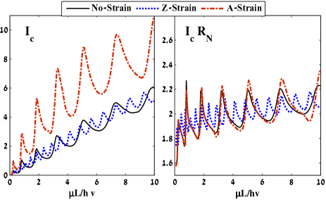
Figure 3: The critical current $I_{c}$ (left panel) and its product with the normal-state resistance $I_{c}R_{N}$ (right panel) as a function of $\mu L/\hbar v$ for a strongly coupled bilayer system. The solid line pertains to a non-strained junction. Here, the same values as for the monolayer system have been used for the tensions, i.e. in the case of $Z$-tension $t_{\vdash}=0.56t_{0},\;t=1.1t_{0}$ while for $A$-tension $t_{\vdash}=0.95t_{0},\;t=0.5t_{0}$ for $s=0.2$.

The behavior of $I_{c}$ and $I_{c}R_{N}$ for strained monolayer graphene-based Josephson junction vs $\mu L/\hbar v$ is shown in Fig.2. The critical current against strain is shown in the inset panel (see Ref.cite:Ribeiro, ). For $A$-strain, we assume $t_{\vdash}=0.95t_{0}$, $t=0.5t_{0}$ ($t_{0}=2.7$ eV for non-strained graphene) and for $Z$-strain $t_{\vdash}=0.56t_{0}$, $t=1.1t_{0}$ which follows when $s=0.2$ cite:Pereira . As seen, the critical current becomes nearly zero at the charge neutrality point for $Z$-strain, whereas the current is enhanced compared to the non-strained case when the strain is applied along the $A$ direction. In effect, the $Z$-strain induces a very small phase-dependent contribution to the Andreev-bound states and the supercurrent vanishes. This suggests a remarkable fact: the supercurrent can be efficiently tuned by means of both the magnitude and the direction of the strain imposed on the system, even at the Dirac point. We have also considered the same model of strain for a bilayer graphene S$\mid$N$\mid$S junction and plot $I_{c}$ and $I_{c}R_{N}$ as a function of $\mu L/\hbar v$ in Fig.3. In this case, it is seen that the critical current tends toward zero as one approaches the Dirac point because of the assumption $t_{\bot}\gg\varepsilon,\Delta$ which influences the evanescent modes cite:paper_delta_F . The obtained normal-state transmission probability $\tau_{n}^{\mathcal{B}}$ is proportional to $\mu$ and hence tends toward zero as one approaches the charge neutrality point. In order to understand these results, one has to consider two facts: i) all transport modes $n$ in the system become evanescent $(k_{n}=iq_{n})$ at the Dirac point and ii) have a transmission probability through the junction given by $\tau_{n}$. In the $Z$- and $A$-strain cases, $\tau_{n}$ decays, respectively, faster and slower than the non-strained graphene as a function of $q_{n}$. In turn, this dictates the magnitude of the contribution of transverse modes to the electron transmission and thus to the discrete Andreev bound state spectrum for the $A$- and $Z$-strains with respect to the non-strained system.

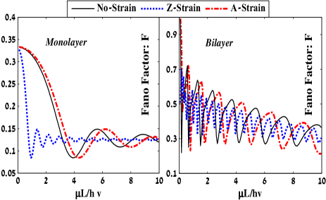
Figure 4: The Fano factor $F$ for both monolayer and bilayer systems with a weakly doped region sandwiched between two heavily doped sides (the normal-state of the mentioned S$\mid$N$\mid$S junction) as a function of $\mu L/\hbar v$. In the scenarios with strain, the same parameters as in Fig.2 and Fig.3 have been used.

We have also calculated the Fano factor (the ratio of noise power and mean current) via the normal transmission probability $\tau_{n}$, defined as $F=\sum^{\infty}_{0}\tau_{n}(1-\tau_{n})/\sum^{\infty}_{0}\tau_{n}$ cite:Tworzydlo . The results for both mono- and bilayer graphene with and without strain are shown in Fig.4. In the non-strained case, we reproduce previous results for monolayer cite:Tworzydlo and bilayer cite:Snyman junctions where a weakly doped middle region is sandwiched between two heavily doped regions cite:Ossipov ; cite:Katsnelson . The scenario with strain has not been considered up to now, and inspection of Fig.4 reveals that the strain influences how $F$ evolves with the doping-level in the middle region. More specifically, in the $Z$-strain case the contribution of the transversal modes is suppressed and therefore the $F$ goes towards saturation faster than the $A$- and non-strained regimes as the doping-degree $\mu$ is increased. The system under tension, however, sustains still the universal value of $F=1/3$ at the Dirac point just as the non-strained monolayer system or diffusive normal metal cite:Tworzydlo ; cite:Snyman . We note that the influence of trigonal warping may be neglected in the monolayer case when the impurity-potential is weak (ballistic regime) tworz_prb_08 . For the bilayer case, the trigonal warping becomes influential in the low-energy regime $|\varepsilon|<0.5\gamma_{1}(v_{3}/v)^{2}$ where a relevant estimate for the parameters is $\gamma_{1}=0.39$ eV and $v_{3}/v=0.1\ll 1$ cite:mccann1 . This yields $|\varepsilon|<2$ meV. However, the influence of strain in the considered bilayer model in this paper becomes most evident at higher doping levels as seen from Fig.3 where the trigonal warping effects can be neglected.

IV Conclusion

In conclusion, we have proposed a novel class of ballistic graphene monolayer/bilayer-based Josephson junctions with mechanical strain. We have derived a general analytical normal transition probability valid for both strained monolayer and bilayer graphene systems. We have demonstrated that the direction of the applied strain to the system near the charge neutrality point can be used to efficiently tune the magnitude of the supercurrent in such a system. In addition, we have considered the Fano factor $F$ in the normal-state of this junction and how it is influenced by strain in the system. In this case, we also find that the direction of the strain is influential with respect to how $F$ depends on the doping-level of the graphene sheet. We believe that these results point towards new perspectives within tunable quantum transport by means of mechanically induced strain. Interesting phenomena may be expected to arise out of the coexistence of proximity induced ferromagnetism and superconductivity in a strained graphene junctions cite:zou .

Appendix A Andreev subgap states

In this appendix, we present more details of our analytical approach used to find the general normal transition probability in Sec. II. We here also examine our analytical expressions for non-strained monolayer case where $s$ is equal to zero. In the graphene monolayer superconducting regions, the right- and left-going quasiparticles are described via the following spinors

$$\left\{\begin{array}[]{c}\Psi_{e^{\pm}}^{S}=(\pm a_{e^{\pm}}^{S}e^{i\beta},e^{i\beta},\pm a_{e^{\pm}}^{S},1)^{T}e^{\pm ik_{e}^{S}L}\\ \Psi_{h^{\pm}}^{S}=(\mp a_{e^{\mp}}^{S},1,\mp a_{e^{\mp}}^{S}e^{i\beta},e^{i\beta})^{T}e^{\mp ik_{h}^{S}L}\end{array}\right..$$ (34)

Similar spinors are obtained when starting with the Hamiltonian Eq. (2) for the strained bilayer case, although they become 1$\times$8 arrays. We focus our attention on the strained monolayer Josephson junctions in this appendix. Matching the wave functions of the superconducting and normal segments at the two interfaces generates the following matrix for reflection and transmission coefficients.

$$\emph{M}=\left(\begin{array}[]{cc}\emph{M}_{11}&\emph{M}_{12}\\ \emph{M}_{21}&\emph{M}_{22}\\ \end{array}\right)$$ (37)

$$\emph{M}_{11}=\left(\begin{array}[]{cccc}-a_{e^{-}}^{S}e^{i\beta}&a_{h^{+}}^{S}&-a_{e^{+}}^{N}&a_{e^{-}}^{N}\\ e^{i\beta}&1&-1&-1\\ -a_{e^{-}}^{S}e^{-i\phi}&a_{h^{+}}^{S}e^{-i(\phi-\beta)}&0&0\\ e^{-i\phi}&e^{-i(\phi-\beta)}&0&0\\ \end{array}\right)\emph{M}_{12}=\left(\begin{array}[]{cccc}0&0&0&0\\ 0&0&0&0\\ a_{h^{+}}^{N}&-a_{h^{-}}^{N}&0&0\\ -1&-1&0&0\\ \end{array}\right)\emph{M}_{21}=\left(\begin{array}[]{cccc}0&0&-a_{e^{+}}^{N}e^{i\hbar k_{e}^{N}L}&a_{e^{-}}^{N}e^{-i\hbar k_{e}^{N}L}\\ 0&0&-e^{i\hbar k_{e}^{N}L}&-e^{-i\hbar k_{e}^{N}L}\\ 0&0&0&0\\ 0&0&0&0\\ \end{array}\right)$$ (50)

$$\emph{M}_{22}=\left(\begin{array}[]{cccc}0&0&a_{e^{+}}^{S}e^{i(\hbar k_{e}^{S}L+\beta)}&-a_{h^{-}}^{S}e^{-i\hbar k_{h}^{S}L}\\ 0&0&e^{i(\hbar k_{e}^{S}L+\beta)}&e^{-i\hbar k_{h}^{S}L}\\ a_{h^{+}}^{N}e^{i\hbar k_{h}^{N}L}&-a_{h^{-}}^{N}e^{-i\hbar k_{h}^{N}L}&a_{e^{+}}^{S}e^{i\hbar k_{e}^{S}L}&-a_{h^{-}}^{S}e^{-i(\hbar k_{h}^{S}L-\beta)}\\ -e^{i\hbar k_{h}^{N}L}&-e^{-i\hbar k_{h}^{N}L}&e^{i\hbar k_{e}^{S}L}&e^{-i(\hbar k_{h}^{S}L-\beta)}\\ \end{array}\right)$$ (55)

To determine the relation between the subgap energy of the quasiparticles and the superconducting phase difference, we use the determinant of M as mentioned in the Sec. II. Previously in this paper, we have considered a heavily doped superconducting regions which dictates normal trajectories of the quasiparticles relative the interfaces inside these regions. In this appendix, we now allow for a moderately doped superconducting region i.e. $\mu^{S}>\varepsilon,\Delta$ and then $\theta_{e}^{S}\approx\theta_{h}^{S}=\gamma\neq 0$. In this regime, we find $\digamma_{1}$, $\digamma_{2}$ and $\digamma_{3}$ factors as follow;

$$\digamma_{1}=\sin(k_{e}^{N}L)\sin(k_{h}^{N}L)(\sin(\gamma)-\sin(\theta))(\sin(\gamma)+\sin(\theta_{A}))-\cos^{2}(\gamma)\cos(\theta)\cos(\theta_{A})\cos(\phi)$$

$$\digamma_{2}=\cos(k_{e}^{N}L)\cos(\gamma)\cos(\theta)\sin(k_{h}^{N}L)(\sin(\gamma)\sin(\theta_{A})+1)$$

$$-\cos(k_{h}^{N}L)\cos(\gamma)\cos(\theta_{A})\sin(k_{e}^{N}L)(\sin(\gamma)\sin(\theta)-1)$$

$$\digamma_{3}=\cos(k_{e}^{N}L)\cos(k_{h}^{N}L)\cos(\theta)\cos(\theta_{A})\cos^{2}(\gamma)+(\sin(\gamma)\sin(\theta)-1)(\sin(\gamma)\sin(\theta_{A})+1)$$

We denote $\theta_{e}=\theta$ and $\theta_{h}=\theta_{A}$. If we apply the short junction approximation to the factors and assume heavily doped superconducting regions i.e. $\gamma\rightarrow 0$, we recover the results of Ref. cite:Titov1, .

References

• (1) K. S. Novoselov, A. k. Geim, S. V. Morozov, D. Jiang, Y. Zhang, S. V. Dubonos, I. V. Grigorieva, and A. A. Firsov, Science 306, 666 (2004); K. S. Novoselov, A. K. Geim, S. V. Morozov, D. Jiang, M. I. Katsnelson, I. V. Grigorieva, S. V. Dubonos, and A. A. Firsov, Nature (London) 438, 197 (2005).
• (2) Y. Zhang, Y.-W. Tan, H. L. Stormer, P. Kim , Nature (London) 438, 201 (2005).
• (3) C. W. J. Beenakker, Phys. Rev. Lett. 97, 067007 (2006).
• (4) M. Titov, A. Ossipov, and C. W. J. Beenakker, Phys. Rev. B75, 045417 (2007)
• (5) J. Tworzydlo, B. Trauzettel, M. Titov, A. Rycerz, and C. W. J. Beenakker, Phys. Rev. Lett. 96, 246802 (2006).
• (6) I. Snyman and C. W. J. Beenakker, Phys. Rev. B75, 045322 (2007).
• (7) A. Ossipov, M. Titov, and C. W. J. Beenakker, Phys. Rev. B75, 241401(R) (2007); S. Gattenlöhner, W. Belzig, and M. Titov, Phys. Rev. B82, 155417 (2010); J. Linder, T. Yokoyama, D. Huertas-Hernando, and A. Sudbø, Phys. Rev. Lett. 100, 187004, (2008).
• (8) M. Titov and C. W. J. Beenakker, Phys. Rev. B74, 041401(R) (2006).
• (9) A.R. Akhmerov and C. W. J. Beenakker, Phys. Rev. B75 045426 (2007).
• (10) N. Levy, S. A. Burke, K. L. Meaker, M. Panlasigui, A. Zettl, F. Guinea, A. H. Castro Neto, and M. F. Crommie, Science 329, 544 (2010).
• (11) N. M. R. Peres, Rev. Mod. Phys. 82, 2673 (2010).
• (12) C. W. J. Beenakker, Phys. Rev. Lett. 66 3056, (1991).
• (13) V. M. Pereira, A. H. Castro Neto and N. M. R. Peres, Phys. Rev. B80, 045401 (2009).
• (14) S.-M. Choi, S.-H. Jhi and Y.-W. Son, Phys. Rev. B81, 081407(R) (2010).
• (15) S.-M. Choi, S.-H. Jhi and Y.-W. Son, Nano Lett. 10 3486 (2010); A. H. Castro Neto, F. Guinea, N. M. R. Peres, K. S. Novoselov and A. K. Geim, Rev. Mod. Phys. 81, 109 (2009); C.-H. Park, L. Yang, Y.-W. Son, M. L. Cohen, and S. G. Louie, Phys. Rev. Lett. 101, 126804 (2008); C.-H. Park and S. G. Louie, Nano Lett. 8, 2920 (2008); A. G. Moghaddam and M. Zareyan, Phys. Rev. Lett. 105, 146803 (2010)..
• (16) C. W. J. Beenakker, Rev. Mod. Phys. 80, 1337 (2008).
• (17) E. McCann and Vladimir I. Falko, Phys. Rev. Lett. 96, 086805 (2006).
• (18) J. Nilsson, A. H. Castro Neto, N. M. R. Peres, and F. Guinea, Phys. Rev. B73, 214418 (2006).
• (19) E. Schrödinger, Sitzber. Preu . Akad. Wiss. 24, 418 (1930).
• (20) E. V. Castro , K. S. Novoselov, S. V. Morozov, N. M. R. Peres, J. M. B. Lopes dos Santos, Johan Nilsson, F. Guinea, A. K. Geim, and A. H. Castro Neto, Phys. Rev. Lett. 99, 216802 (2007).
• (21) T. Ludwig, Phys. Rev. B75, 195322 (2007).
• (22) J.C. Cuevas and A. Levy Yeyati, Phys. Rev. B74, 180501(R) (2006).
• (23) We define $a_{x}=(1+s)c_{0}/2$, $a_{y}=c_{0}(1-ps)/2$ so that the $Z$-strain leads $\overrightarrow{\sigma_{1}}=\hat{x}a_{x}\sqrt{3}-\hat{y}a_{y}$, $\overrightarrow{\sigma_{2}}=-\hat{x}a_{x}\sqrt{3}-\hat{y}a_{y}$, $\overrightarrow{\sigma_{3}}=\hat{y}2a_{y}$ and then for the $A$-strain, $\overrightarrow{\sigma_{1}}=\hat{x}a_{y}\sqrt{3}-\hat{y}a_{x}$, $\overrightarrow{\sigma_{2}}=-\hat{x}a_{y}\sqrt{3}-\hat{y}a_{x}$, $\overrightarrow{\sigma_{3}}=\hat{y}2a_{x}$ . Also $t_{i}=t_{0}e^{-3.37(\mid\overrightarrow{\sigma_{i}}\mid)/c_{0}-1}$, $c_{0}=0.142\AA$ is distance of two C atoms in the non-strained graphene, $p=0.165$ is Poisson s ratio for graphite and $s=0.2$ which is fixed throughout our calculations, represents the strength of applied tension to the system. The assumed tension strength is near the gap threshold value, i.e. $s=0.23\sim\%20$ (see Ref.cite:Pereira, ).
• (24) B. Soodchomshom, Physica B, 406, 614 (2011); B. Soodchomshom, arXiv:1011.1617 (unpublished).
• (25) R. M. Ribeiro, V. M. Pereira, N. M. R. Peres, P. R. Briddon and A. H. Castro Neto, New J. Phys. 11, 115002 (2009).
• (26) The evanescent modes appear in an interval of order $\Delta E_{F}\simeq(\hbar v)^{2}/t_{\bot}L^{2}$ cite:Snyman . Our results in the bilayer case are restricted to the regime $\mu>\Delta$ due to the choice of wavefunction.
• (27) M. I. Katsnelson, Eur. Phys. J. B 51, 157 (2006).
• (28) F. d. Juan, A. Cortijo, and M. A. H. Vozmediano, Phys. Rev. B76, 165409 (2007); N. M. R. Peres, Rev. Mod. Phys. 82, 2673 (2010)
• (29) J. Tworzydlo, C. W. Groth2, and C. W. J. Beenakker, Phys. Rev. B78, 235438 (2008).
• (30) Q. Liang, Phys. Rev. Lett. 101, 187002 (2008); A. Black-Schaffer and Sebastian Doniach, Phys. Rev. B78, 024504 (2008); J. Linder, A. M. Black-Schaffer, T. Yokoyama, S. Doniach, and A. Sudbø, Phys. Rev. B80, 094522 (2009); I. Hagymasi, A. Kormanyos, and J. Cserti, Phys. Rev. B82, 134516 (2010).
• (31) K. Halterman, O. T. Valls and M. Alidoust, arXiv:1105.4140 (unpublished)
• (32) J. Linder, Y. Tanaka, T. Yokoyama, A. Sudbø, and N. Nagaosa, Phys. Rev. B81, 184525 (2010); J. Linder, Y. Tanaka, T. Yokoyama, A. Sudbø, and N. Nagaosa, Phys. Rev. Lett. 104, 067001 (2010).
• (33) J. F. Zou and G. J. Jin, Appl. Phys. Lett. 98, 12, 122106 (2011).
• (34) T. W. Tombler, C. Zhou, L. Alexseyev, J. Kong, H. Dai, L. Liu, C. S. Jayanthi, M. Tang, S. Wu , Nature 405, 769 (2000).
• (35) L. Yang and J. Han, Phys. Rev. Lett. 85, 154 (2000).
• (36) E. D. Minot, Y. Yaish, V. Sazonova, J. Park, M. Brink, and P. L. McEuen, Phys. Rev. Lett. 90, 156401 (2003).
• (37) T. M. G. Mohiuddin, A. Lombardo, R. R. Nair, A. Bonetti, G. Savini, R. Jalil, N. Bonini, D. M. Basko, C. Galiotis, N. Marzari, K. S. Novoselov, A. K. Geim, and A. C. Ferrari, Phys. Rev. B79, 205433 (2009).
• (38) K. S. Kim, Y. Zhao, H. Jang, S. Y. Lee, J. M. Kim, K. S. Kim, J.-H. Ahn, P. Kim, J.-Y. Choi, B. H. Hong , Nature 457, 706 (2009).
• (39) N. Ferralis, R. Maboudian and C. Carraro, Phys. Rev. Lett. 101, 156801 (2008).
• (40) M. Huang, H. Yan, C. Chen, D. Song, T. F. Heinz and J. Hone, Proc. Nat. Acad. Sci. 106, 7304 (2009).
• (41) A. D. Beyer, M. W. Bockrath, C.-N. Lau, and N.-C. Yeh, Nano Lett. 9, 2542 (2009).
• (42) Y. Zhang, T.-T. Tang, C. Girit, Z. Hao, M. C. Martin, A. Zettl, M. F. Crommie, Y. R. Shen, F. Wang , Nature 459, 820 (2009).
• (43) K. F. Maik, C. H. Lui, J. Shan, and T. F. Heinz, Phys. Rev. Lett. 102, 256405 (2009).
• (44) Z. Q. Li, E. A. Henriksen, Z. Jiang, Z. Hao, M. C. Martin, P. Kim, H. L. Stormer, and D. N. Basov1, Phys. Rev. Lett. 102, 037403 (2009).
• (45) J. B. Oostinga, H. B. Heersche, X. Liu, A. F. Morpurgo, L. M. K. Vandersypen , Nature Mat. 7, 151 (2008).
• (46) A. B. Kuzmenko, L. Benfatto, E. Cappelluti, I. Crassee, D. van der Marel, P. Blake, K. S. Novoselov, and A. K. Geim, Phys. Rev. Lett. 103, 116804 (2009).