Tracing the gas to the virial radius (${\rm R_{100}}$) in a fossil group

Abstract

We present a Chandra, Suzaku and Rosat study of the hot Intra Group Medium (IGrM) of the relaxed fossil group/ poor cluster RXJ 1159+5531. This group exhibits an advantageous combination of flat surface brightness profile, high luminosity and optimal distance, allowing the gas to be detected out to the virial radius (${\rm R_{vir}}$$\equiv R_{108}=$1100 kpc) in a single Suzaku pointing, while the complementary Chandra data reveal a round morphology and relaxed IGrM image down to  kpc scales. We measure the IGrM entropy profile over $\sim$3 orders of magnitude in radius, including 3 data bins beyond $\sim 0.5$${\rm R_{200}}$ that have good azimuthal coverage ($>$30%). We find no evidence that the profile flattens at large scales ($>$${\rm R_{500}}$), and when corrected for the enclosed gas fraction, the entropy profile is very close to the predictions from self-similar structure formation simulations, as seen in massive clusters. Within ${\rm R_{vir}}$, we measure a baryon fraction of $0.17\pm 0.02$, consistent with the Cosmological value. These results are in sharp contrast to the gas behaviour at large scales recently reported in the Virgo and Perseus clusters, and indicate that substantial gas clumping cannot be ubiquitous near ${\rm R_{vir}}$, at least in highly evolved (fossil) groups.

1. Introduction

Galaxy groups (defined here as bound systems with virial masses, ${\rm M_{vir}}$, in the range $\sim 10^{13}$–$10^{14}$${\rm M_{\odot}}$) are essential ingredients in the assembly of structure within the Universe. Locally $\sim$30% of galaxies are found in groups that are less massive than $10^{14}$${\rm M_{\odot}}$ (Eke et al., 2004). Systems of this mass range have been implicated as key sites in both efficient star formation (Springel & Hernquist, 2003), and the morphological transformation of galaxies (Zabludoff & Mulchaey, 1998). Typically the dominant baryonic component is, however, an extended, hot gas halo, that can contain $\mathrel{\hbox to0.0pt{\lower 3.0pt\hbox{$\sim$}\hss}\raise 2.0pt\hbox{$>$}}$ 70% of the baryons at ${\rm M_{500}}$$\mathrel{\hbox to0.0pt{\lower 3.0pt\hbox{$\sim$}\hss}\raise 2.0pt\hbox{$>$}}$ $5\times 10^{13}$${\rm M_{\odot}}$ (Giodini et al., 2009). Such a massive hot gas halo can make them both luminous X-ray sources, and, potentially, targets for detection in large numbers by future Sunyaev-Zeldovich surveys (Haiman et al., 2001).

X-ray observations provide the best means for studying emission from the hot gas in groups. Of particular interest is the entropy proxy, $S=n_{e}^{-2/3}kT$ (where $n_{e}$ is the electron number density, $k$ is Boltzmann’s constant and T is the temperature), which is related to the specific entropy through a logarithm and constant offset. If purely gravitational processes shape the energetics of the gas, self-similar structure formation simulations predict an entropy profile that rises with radius, r, such that $S\propto T_{0}r^{1.1}$, where $T_{0}$ is a characteristic temperature (Tozzi & Norman, 2001; Voit et al., 2005; Kaiser, 1986). Observations of galaxy clusters in fact reveal lower-mass objects to be systematically offset upwards from this relation, but approaching it by $\sim$${\rm R_{500}}$ (e.g. Ponman et al., 2003; Pratt et al., 2010). This indicates nongravitational energy injection, likely a consequence of preheating of the gas in filaments prior to accretion, or feedback due to star formation or a central AGN (Voit & Ponman, 2003; Voit & Donahue, 2005; Ponman et al., 2003). The fine balance between these different processes should affect both the shape and normalization of the entropy proxy profile, making it a potentially powerful diagnostic (e.g. Borgani et al., 2005; McCarthy et al., 2010), especially at the group scale, where these effects should be comparatively more important. Recent Chandra and XMM observations of relaxed groups have revealed complex entropy profiles that flatten at large ($\mathrel{\hbox to0.0pt{\lower 3.0pt\hbox{$\sim$}\hss}\raise 2.0pt\hbox{$>$}}$ 0.1${\rm R_{500}}$) and small scales, albeit with some scatter (Gastaldello et al., 2007a; Mahdavi et al., 2005; Finoguenov et al., 2007; Humphrey et al., 2008; Sun et al., 2009; Cavagnolo et al., 2009; Johnson et al., 2009; Flohic et al., 2011), possibly indicating that both star formation and AGN feedback are important (Voit & Donahue, 2005; McCarthy et al., 2010).

Feedback also shapes the enclosed gas fraction (${\rm f_{gas}}$) profiles of groups and clusters, which are found to rise with radius (Allen et al. 2002; Vikhlinin et al. 2006; G07; Sun et al. 2009), but with groups containing a systematically smaller fraction of their gas at small scales (e.g. Fig 11 of Humphrey et al. 2011, hereafter H11). Assuming they can be converted into a reliable estimate for the total (initial) baryon fraction in the cluster (${\rm f_{b}}$), ${\rm f_{gas}}$ measurements are a powerful cosmological tool, used either directly (White et al., 1993; Allen et al., 2002), or in employing the gas mass as a virial mass proxy (e.g. Voevodkin & Vikhlinin, 2004). Massive clusters are preferred in this analysis since ${\rm f_{gas}}$ measured at these scales should be closer to ${\rm f_{b}}$ than in poor clusters or groups. Still, systems with masses as low as $\sim 2\times 10^{14}$${\rm M_{\odot}}$ (Allen et al., 2008), or even lower (Voevodkin & Vikhlinin, 2004) are routinely used. Translating into ${\rm f_{b}}$ the ${\rm f_{gas}}$ values measured at scales far smaller than the virial radius, ${\rm R_{vir}}$ (typically at $\sim$${\rm R_{2500}}$), involves a number of assumptions that have yet to be robustly verified, especially in lower mass halos (e.g. Arnaud, 2005). Intriguingly, for most of the group-scale objects studied by Gastaldello et al. (2007b, hereafter G07), extrapolating ${\rm f_{gas}}$ outside the field of view yielded global ${\rm f_{b}}$ constraints consistent with the Universal baryon fraction (0.17: Dunkley et al., 2009; Komatsu et al., 2011), in accord with the idea that X-ray bright groups are baryonically closed (Mathews et al., 2005). Nevertheless, this extrapolation was subject to significant systematic uncertainty.

To date, most observations of the gas in groups and clusters have been restricted to within $\sim$${\rm R_{500}}$, and typically much smaller scales are attained. For example, ${\rm R_{500}}$ was only reached for 11 of the 43 systems studied in the current largest group sample (Sun et al., 2009). In groups at these scales, ${\rm f_{gas}}$ is still only $\sim$0.07, in contrast to $\sim$0.11 for clusters. Given the low, stable background for the Suzaku XIS instrument, recent work has begun to push measurements of the ICM in clusters out to $\sim$${\rm R_{200}}$, or beyond, but a coherent picture has not yet emerged. While some studies have found consistency with model predictions (Reiprich et al., 2009; Hoshino et al., 2010), deviations from hydrostatic equilibrium (Bautz et al., 2009), temperature asymmetries associated with large-scale structure (Kawaharada et al., 2010) and, in three systems, an unexpected flattening of the entropy proxy profile outside $\sim$${\rm R_{500}}$ (PKS0745-191: George et al. 2009; Perseus: Simionescu et al. 2011; Virgo: Urban et al. 2011), have been seen. Simionescu et al. and Urban et al. (see also Nagai & Lau, 2011) attributed the entropy flattening, and associated over-estimate of ${\rm f_{gas}}$, to putative clumpiness of the ICM in the outskirts of the cluster, leading to a systematically biased gas density measurement.

Given the lack of a consistent story in the outskirts of clusters, the ubiquity of a clumpy ICM remains to be determined. The azimuthal temperature variations in Perseus (Simionescu et al., 2011) and the large-scale asymmetries in the X-ray image of Virgo (Böhringer et al., 1994) indicate that these systems are not relaxed at large scales, consistent with ongoing formation. This could give rise to deviations from sphericity (complicating the deprojection) or local hydrostatic equilibrium (hence an underestimate of the gravitating mass, and an over-estimate of ${\rm f_{gas}}$), and local distortions in the entropy profile. On account of the proximity of these clusters, only a small fraction of the outer annuli were imaged in these studies, so it is unclear whether such large effects would be seen in azimuthally averaged profiles. An additional concern is the need to minimize sources of systematic uncertainty in this background-dominated regime (e.g., Reiprich et al. 2009, Bautz et al. 2009, H11). Eckert et al. (2011) demonstrated that the Rosat PSPC surface brightness profile of PKS0745-191 disagrees at 7.7-$\sigma$ with the Suzaku density profile inferred by George et al. (2009). They attributed the discrepancy to systematic errors in the George et al. background treatment. In the outermost bins, the deprojection procedure adopted by Urban et al. (2011) and Simionescu et al. (2011) depends sensitively on the correct modelling of projected emission from regions outside the field of view. Furthermore, while Simionescu et al. attempted to mitigate the scattered light contamination from the cluster core, it is unclear how sensitive their results were to this correction. Similarly, the XMM-Newton profiles of Urban et al. were sensitive to the treatment of the background.

In this paper, we present a joint Chandra and Suzaku study (carefully cross-checked with the archival Rosat data) of the very relaxed galaxy group RXJ 1159+5531, allowing, for the first time in a system with a mass as low as $\sim 10^{14}$${\rm M_{\odot}}$, the gas to be traced to scales as large as the virial radius, $R_{108}$. A single, giant elliptical galaxy dominates the stellar light, making it a prototypical “fossil group” (Vikhlinin et al., 1999) and implying a highly evolved (i.e. relaxed) dynamical state (Ponman et al., 1994). The optimal combination of distance ($z=0.081$), mass (${\rm R_{vir}}$$=12$′) and high surface brightness (such that gas is already detected to $\sim$${\rm R_{500}}$ with Chandra: Vikhlinin et al. 2006; G07; Sun et al. 2009), make it possible to measure the gas to ${\rm R_{vir}}$ in a single, modest (85 ks) Suzaku pointing.

The group was observed with the X-ray centroid slightly offset (by 5′) from the Suzaku optical axis, to enable coverage out to $\sim$12′, while minimizing the complications of stray-light from having the X-ray peak outside the field of view. Although this configuration limited the number of radial bins we can study, by combining the Chandra and Suzaku data, we were able to achieve $\sim$3 spatial bins outside $\sim 0.5$${\rm R_{200}}$, with $\mathrel{\hbox to0.0pt{\lower 3.0pt\hbox{$\sim$}\hss}\raise 2.0pt\hbox{$>$}}$ 30% azimuthal coverage, in comparison with $\sim$6 bins, and $\sim$15% coverage in the $\sim$3 times longer Suzaku exposure of Perseus (Simionescu et al., 2011). In conjunction with the archival Chandra data, we were able to measure the gas properties over almost three orders of magnitude in radius.

Previous studies of RXJ 1159+5531, based on the Chandra data (Vikhlinin et al. 2006; G07; Sun et al. 2009), have reported conflicting parameterizations of the gravitating mass profile. Adopting the popular Navarro-Frenk-White (NFW: Navarro et al., 1997) profile (plus, in the case of G07, a baryonic component), ${\rm M_{500}}$ inferred from these studies has varied significantly from $\sim 6\times 10^{13}$–$10^{14}$${\rm M_{\odot}}$, and the corresponding NFW concentration parameter from $\sim$1.7–5.6, which remains a puzzle (see § 4.2). The addition of new data at large scales should help pin down the mass profile more precisely, particularly if the scale radius were as high as found by Vikhlinin et al. (400 kpc). In this paper, we employed the “forward-fitting” mass analysis techniques outlined in H11, which enable finer control of systematic uncertainties than more traditional methods (Buote & Humphrey, 2011a).

We assumed a flat cosmology with $H_{0}=70{\rm km\ s^{-1}}$ and $\Omega_{\Lambda}=0.7$. We adopted $R_{108}$ as the virial radius (${\rm R_{vir}}$), based on the approximation of Bryan & Norman (1998) for the redshift of RXJ 1159+5531. Unless otherwise stated, all error-bars represent 1-$\sigma$ confidence limits (which, for our Bayesian analysis, implies the marginalized region of parameter space within which the integrated probability is 68%).

2. Data Reduction and Analysis

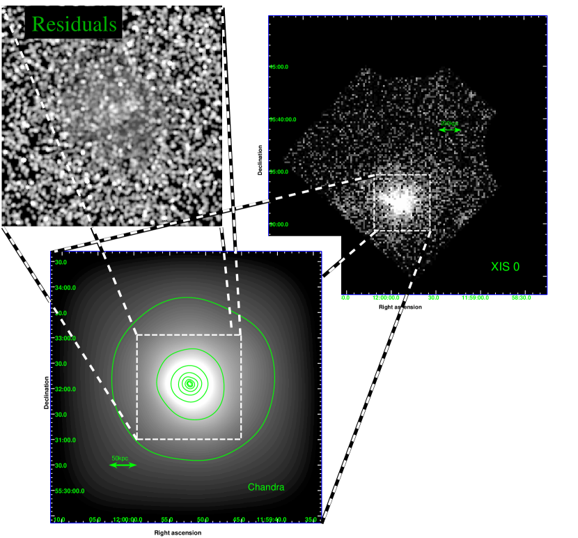
Figure 1.— Suzaku XIS0 (top right) and Chandra (bottom left) images of RXJ 1159+5531 . The apparent asymmetries in the XIS0 image are due to the asymmetric point spread function of the telescope, rather than the intrinsic shape of the source. The Chandra image has been cleaned of point sources and mildly smoothed. The smoothing scale varied from $\sim$1″ at the smallest scales, to $\sim$1.1′ (100 kpc) at the outer part of the image (see text). At the top left, we show a “residual significance” image (see text) of the centre of the group, indicating deviations from a smooth model fit to the (Chandra) X-ray isophotes. There is no obvious large-scale feature in this map, indicating the system is largely relaxed.

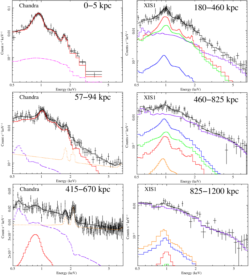
Figure 2.— Representative Chandra and Suzaku XIS1 spectra for RXJ 1159+5531, shown (Chandra) without background subtraction, or (Suzaku) with the instrumental background subtracted. In addition to the data, we show the best-fitting model, folded through the instrumental response (solid black line), along with the decomposition of this model into its various components. For the Chandra data, we show the hot gas contribution (solid red line), the composite emission from X-ray binaries (dash-dot magenta line), the instrumental background (dotted orange) and the cosmic X-ray background (dashed purple line). For the XIS1 data, we show the hot gas emission from each annulus as solid lines (red, green, blue and orange indicating, respectively, the 0–2′, 2–5′, 5–9′and 9–13′ apertures, respectively) , sky background (using the same colour scheme as for Chandra). For Chandra, the background is dominated by the instrumental component, whereas for Suzaku, which has a lower instrumental background but is less able to resolve the cosmic component into individual point sources, the cosmic component dominates.

2.1. Chandra

The region of sky containing RXJ 1159+5531 was imaged by the ACIS instrument aboard Chandra on two separate occasions. We consider here only the deep data taken in the ACIS-S configuration (Observation ID 4964; beginning on Feb 11 2004). A shallower ACIS-I observation was also available, but to simplify the analysis (in particular, the background modelling), we chose not to include it in our study. The data-reduction was carried out as described in H11, using the CIAO 4.1 and Heasoft 6.8 software suites, in conjunction with the Chandra calibration database (Caldb) version 4.1.2. Briefly, the data were reprocessed from the “level 1” events files, following the standard data reduction threads. Periods of high background were identified by eye in the lightcurve from a low surface-brightness region of the CCDs and data from these intervals were excised, leaving a total exposure of 75 ks. Point sources were detected in the 0.3–7.0 keV image with the wavdetect CIAO task, which was supplied a 1.7 keV exposure map to minimize spurious detections at chip boundaries. The detection threshold ($10^{-6}$) guaranteed $\mathrel{\hbox to0.0pt{\lower 3.0pt\hbox{$\sim$}\hss}\raise 2.0pt\hbox{$<$}}$ 1 spurious source per CCD. All detected sources were confirmed visually, and appropriate elliptical regions containing $\sim 99$% of the source photons were generated.

In Fig 1, we show a smoothed, flat-fielded Chandra image, having removed the point sources with the algorithm outlined in Fang et al. (2009). The image was smoothed with a Gaussian kernel, the width of which varied with distance from the nominal X-ray centroid according to an arbitrary powerlaw, ranging from $\sim$1″ at the centre of the image to $\sim$1′ at its edge. The image is smooth and very round, consistent with the relaxed morphology expected for a fossil system. To search for more subtle structure, we used dedicated software to fit an elliptical beta model (with constant ellipticity) to the central 2′-wide portion of the unsmoothed (flat-fielded) image. In Fig 1, we plot $(data-model)^{2}/model$, corresponding (approximately) to the $\chi^{2}$ residuals from this fit. To bring out the structure, we smoothed this image with a Gaussian kernel of width 3 pixels. There is weak evidence of a small ($\sim$4″), coherent structure in the residuals within the central ($\sim$10 kpc) region, which may imply a small depression in the surface brightness (by $\sim$20–30%). The formal significance of this feature depends sensitively on prior information (in particular, the region of the image over which one searches for structures; e.g. Kaastra et al., 2006). Still, even if the feature is real, it should not give rise to a significant error in the recovered, azimuthally averaged mass profile (see Buote & Humphrey, 2011a; Churazov et al., 2008). Aside from this modest feature, the overall lack of significant, coherent residuals indicates that the X-ray image is very relaxed.

Spectra were extracted in a series of contiguous, concentric annuli centred at the X-ray centroid. The widths of the annuli were chosen to contain approximately the same number of background-subtracted counts, while ensuring sufficient photons for useful spectral analysis. The resulting annuli had widths larger than $\sim$3″, which is sufficient to prevent spectral mixing between adjacent annuli on account of the finite spatial resolution of the mirrors. Data in the vicinity of point sources and chip gaps were excluded. We extracted spectra from all the active chips (excluding S4, which suffers from noise). Appropriate count-weighted spectral response matrices were generated for each annulus with the standard CIAO tools mkwarf and mkacisrmf. Representative spectra, without background subtraction, are shown in Fig 2.

Spectral-fitting was carried out in the energy band 0.5–7.0 keV, using Xspec vers. 12.5.1n, by minimizing the C-statistic to mitigate biases that arise (even in the high-count regime) when using the standard $\chi^{2}$ approximations for Poisson-distributed data (Humphrey et al., 2009b). To aid convergence, we rebinned the spectra to ensure at least 20 photons per bin. The data in all annuli were fitted simultaneously, to enable the source and background components to be modelled at the same time. In keeping with H11 and Gastaldello et al. (2007b), we modelled the projected (rather than the deprojected) source emission in each annulus as coming from a single APEC plasma model with variable abundances, modified by foreground Galactic absorption (Dickey & Lockman, 1990). We allowed the total abundance of Fe (${\rm Z_{Fe}}$) and the abundance ratios with respect to Fe of the elements O, Ne, Mg, Si and Ni to vary in each annulus. The abundance of He, and the abundance ratios of the other elements were fixed to 1 Solar (Asplund et al., 2004). To improve S/N, we tied ${\rm Z_{Fe}}$ between the outermost two annuli, and constrained the abundance ratios to be the same in all annuli.

To account for emission from undetected LMXBs in the central galaxy, we included an additional 7.3 keV bremsstrahlung component. Since the number of X-ray point sources is approximately proportional to the stellar light (e.g. Humphrey & Buote, 2008), the relative normalization of this component between each annulus was fixed to match the relative K-band luminosity in the matching regions, which we measured from the 2MASS image. This component is only important in the very central region ($\mathrel{\hbox to0.0pt{\lower 3.0pt\hbox{$\sim$}\hss}\raise 2.0pt\hbox{$<$}}$ 20 kpc) of the system.

To accommodate the background, we included additional spectral components in our fits. Specifically, we included two (unabsorbed) APEC components (kT=0.07 keV and 0.2 keV) and an (absorbed) powerlaw component ($\Gamma=1.41$; De Luca & Molendi 2004). The normalization of each component within each annulus was assumed to scale with the extraction area, but the total normalizations were fitted freely. We discuss the possible impact of an additional, “Solar wind charge exchange” background component in § 6.2.1. To account for the instrumental background, we included a number of Gaussian lines and a broken powerlaw model, which were not folded through the ARF. We included separate instrumental components for the front- and back-illuminated chips, and assumed that the normalization of each component scaled with the area of the extraction annulus which overlapped the appropriate chips. The normalization of each component, and the shape of the instrumental components, were allowed to fit freely. We included two Gaussian lines (at 1.77 and $\sim$2.2 keV), the intrinsic widths of which were fixed to zero. The energies of the $\sim$2.2 keV lines were allowed to fit freely, as were as the normalizations of all the components. To verify the fit had not become trapped in a local minimum, we explored the local parameter space by stepping individual parameters over a range centred around the best-fitting value (analogous to computing error-bars with the algorithm of Cash, 1976). The covariance matrix (which contains the error bars) was computed via the efficient Monte Carlo technique outlined in Humphrey et al. (2006), and we carried out 250 error simulations.

The best-fitting models are shown in Fig 2 for a representative selection of spectra. While the instrumental background is clearly significant at high energies ($\mathrel{\hbox to0.0pt{\lower 3.0pt\hbox{$\sim$}\hss}\raise 2.0pt\hbox{$>$}}$ 2 keV), only in the outermost annulus does the source signal fall below the background level. Nevertheless, given the optimal temperature of the gas ($\simeq$1 keV), the Fe L-shell peak is still visible as a small “bump” in the spectrum at $\sim$0.9 keV, enabling the gas temperature and density to be constrained (this is similar to the outermost annuli of NGC 5044, studied by Buote et al. 2004).

2.2. Suzaku

The region of sky containing RXJ 1159+5531 was imaged by Suzaku beginning on Feb 5 2009 (observation ID 804051010), with three of the XIS units operating. Data-reduction was performed using the Heasoft 6.8 software suite, in conjunction with the XIS calibration database (Caldb) version 20090925. To ensure up-to-date calibration, the unscreened data were re-pipelined with the aepipeline task and analysed following the standard data-reduction guidelines. Since the data for each instrument were divided into differently telemetered events file formats, we converted the “$5\times 5$” formatted data into “$3\times 3$” format, and merged them with the “$3\times 3$” events files. The lightcurve of each instrument was examined for periods of anomalously high background, but no significant amount of data was found to be contaminated in this way, leaving 85 ks of total “cleaned” exposure time. 85 ks total exposure time survived flare cleaning. In Fig 1, we show the 0.5–7.0 keV image for the XIS0 detector, excluding data in the vicinity of the calibration sources. By visual inspection of the images for all three active detectors, we found only 1 bright point-source (coinciding with one of the calibration sources in the XIS0 image). In subsequent analysis, we excluded a circular region of 2.5′ radius, centred on this source (which should eliminate $\mathrel{\hbox to0.0pt{\lower 3.0pt\hbox{$\sim$}\hss}\raise 2.0pt\hbox{$>$}}$ 90% of the source photons from contaminating any spectra).

Since RXJ 1159+5531 was slightly offset from the centre of the field of view, it was possible to extract spectra out to scales of $\sim$13′ from the single, pointed observation. Therefore, spectra were extracted in four concentric annuli (0–2′, 2–5′, 5–9′ and 9–13′), centred at the nominal position of RXJ 1159+5531 in the field of view of each instrument. Due to the large field of view of Suzaku, our spectral extraction regions actually achieve $\sim$55–60% azimuthal coverage in the 5–9′ aperture, and $\sim$27% in the 9–13′ region. Data in the vicinity of the calibration sources and the identified point sources were excluded. For each spectrum, we generated an associated redistribution matrix file (RMF) using the xisrmfgen tool and an estimate of the instrumental background with the xisnxbgen task. Ancillary response files (ARFs) were generated for each spectrum with the xissimarfgen tool (Ishisaki et al., 2007), which models the telescope’s optics through ray-tracing. Since the point-spread function of the telescope is very large ($\sim$2′ half power diameter), even with such large apertures it is necessary to account for spectral mixing between each annulus. We did this by employing the algorithm described in H11.

We modelled the spectrum in each annulus as the sum of source plus sky background components. The instrumental background (which is not the dominant background component; H11) was subtracted directly, using the model generated with the xisnxbgen task. For the source, we included an APEC component, for which the Fe abundance and abundance ratios of other species were allowed to vary (as for the Chandra data). The abundance ratios were tied between all annuli, and ${\rm Z_{Fe}}$ was tied between the outermost two annuli. In the central bin, we also included a 7.3 keV bremsstrahlung component, to account for possible LMXBs in the central galaxy. For this component, we obtained a total X-ray luminosity per unit K-band optical light of $L_{X,LMXB}/L_{K}=2.7\pm 3.9\times 10^{29}erg\ s^{-1}L_{\odot}^{-1}$, in good agreement with the Chandra result of $6.0\pm 1.9\times 10^{29}erg\ s^{-1}L_{\odot}^{-1}$. This self-consistency gives us confidence in our treatment of the background (described below), and the lack of bright source contamination in the Suzaku field. This ratio is also marginally consistent with the mean scaling determined from local galaxies (Humphrey et al., 2008).

The Chandra data reveals a strong temperature gradient within the central $\sim$2′. Since we can generally approximate the integrated spectrum of a region in which there is a temperature gradient by the sum of two APEC components (Buote, 1999; Buote et al., 2003), we added a second APEC component in the central bin. Although we did not consider the fitted temperature or density in this bin in our subsequent analysis, it was still necessary to fit a reasonably accurate model to the data, as some fraction of the photons from this region are scattered into the surrounding annuli. The spectra from all instruments were fitted simultaneously, allowing additional multiplicative constants in the fit to enable the relative normalization of the model for each instrument to vary with respect to the XIS 0.

We found that this model was able to fit the data well. We show in Fig 2 representative spectra for the XIS1 instrument, showing various model components. As is immediately clear, mixing between annuli is significant. Furthermore, the data are clearly background-dominated in the outermost annulus (while the source and background are comparable in the 6–10′ region). Nevertheless, given the $\sim$keV temperature of the gas, the Fe L-shell peak is still clearly visible over the cosmic X-ray background component (§ 5), and so the gas properties can be measured with reasonable precision.

2.3. Rosat

RXJ 1159+5531 was observed serendipitously by Rosat in the outskirts ($\sim$17′ off-axis; $\sim$2.5′ inside the support-ring structure) of a pointed PSPC observation (observation ID 700055n00). Given its relatively poor spatial resolution and limited energy pass-band, we only required to measure the Rosat surface brightness profile, centred at the source (see § 4.5 for more details). We do not expect much extended emission from the principal target of the observation, an unrelated, foreground Sy1 galaxy (NGC 3998). Therefore, we extracted the surface brightness profile of RXJ 1159+5531 out to scales of $\sim$25′ ($\sim 2$${\rm R_{vir}}$). To prepare the data, we followed the standard Rosat data-reduction recipe (see, for example Fang et al., 2009). A full field of view image with 15″ pixel size was generated in the 0.42–2.0 keV band, and the corresponding exposure maps were generated with the pcexpmap task. Point sources were detected with the wavdetect CIAO task to search for structure at scales of 1, 2, 4 and 8 pixels, and supplied with the exposure map to minimize spurious detections at the image boundaries. The detection threshold was set to $10^{-6}$, implying $\mathrel{\hbox to0.0pt{\lower 3.0pt\hbox{$\sim$}\hss}\raise 2.0pt\hbox{$<$}}$ 0.1 spurious detections per image, and all point sources were visually confirmed. We used the ao and castpart Heasoft tasks to generate, respectively, the scattered Solar X-ray background and the particle background contribution, which were then subtracted from the image. The surface brightness profile was generated in concentric annuli from the flat-fielded image, excluding data from the vicinity of any detected point source and, to maximize the ability to identify and exclude point sources, all photons not inside the shadow of the inner PSPC support ring. We discuss the surface brightness analysis in detail in § 4.5.

3. Spectral fitting results

3.1. Metal abundances

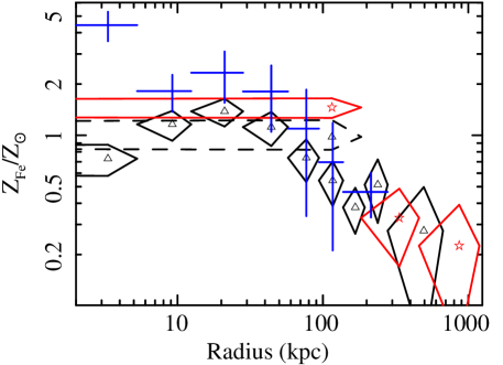
Figure 3.— Projected Fe abundance profile, measured with Chandra (triangles) and Suzaku (stars). The dashed line indicates the Chandra abundance measured in same region as the central Suzaku bin. Note the overall good agreement between Chandra and Suzaku. We also overlay (crosses) the deprojected abundance profile measured with Chandra, including a second temperature component in the innermost bin. Note that the central dip seen in the projected profile is absent in this case.

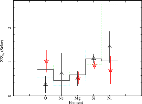
Figure 4.— Abundance ratios with respect to Fe, expressed relative to the Solar ratios (Asplund et al., 2004). Chandra data are marked with triangles, and Suzaku data with stars. The solid line is the best-fit model ($\chi^{2}$/dof=5.7/8) where the enrichment comes from SNIa and SNII, assuming the WDD2 SNIa yields from Nomoto et al. (1997b) and the SNII yields from Nomoto et al. (1997a). The SNIa enrichment fraction is $0.82\pm 0.05$. For reference, we also show the best fits with the W7 (green dashed line) and WDD1 (blue dotted line) SNIa yields, neither of which are formally acceptable.

In Fig 3, we show the projected abundance profile, which is centrally peaked, as expected for a relaxed galaxy group and consistent with a picture in which metal enrichment is facilitated by mass-loss from stars and supernovae in the central galaxy (Mathews & Brighenti, 2003). There is good agreement between the profiles measured outside $\sim$100 kpc with Chandra and Suzaku, supporting our treatment of these data. To effect a comparison within the central 2′, where there is a strong abundance gradient revealed by Chandra, but only a single Suzaku data-bin, we extracted a single Chandra spectrum for this region, and fitted it with the same model as the Suzaku data. The best-fitting ${\rm Z_{Fe}}$ (shown on Fig 3) was consistent (within $\sim$1.5-$\sigma$) with the Suzaku measurement. The good agreement over the entire radial range is encouraging, and suggests that our treatment of the spectral mixing between the Suzaku annuli is approximately correct.

We note the slight dip in the central Chandra bin, similar to features that have been reported in some other galaxy groups and clusters. Still, if hot gas components with a range of different temperatures are found along the line-of-sight to the central annulus, the measured ${\rm Z_{Fe}}$ may be systematically under-estimated due to the “Fe bias” (Buote & Fabian, 1998; Buote, 2000b). Such a situation could arise either due to projection effects, or if there is a strong temperature gradient within that annulus. To investigate this, we carried out a deprojection analysis (see H11, or § 6.4 of this paper, for a detailed description of the deprojection procedure), and, furthermore, included an additional APEC component within the cental bin, with abundances tied to those of the other component. Since the deprojection procedure tends to increase the error-bars on the measured quantities, we found it necessary to fix the abundance outside $\sim$400 kpc to 0.2 Solar (consistent with the projected results). We found that the second hot gas component was formally required in the central bin (the improvement in the C-statistic was 13.7 for a difference of 2 degrees of freedom when it was added); the two temperatures in this bin were $1.29\pm 0.23$ keV and $0.72\pm 0.17$keV, consistent with a continuing temperature decline in the group’s centre, although it may also reflect deficiencies in the deprojection procedure.

The deprojected ${\rm Z_{Fe}}$ profile is shown in Fig 3, and it also exhibits a centrally-peaked shape and, significantly, no evidence of a central abundance dip. This strongly suggests that the feature seen in the central bin of the projected data is simply an artefact of the Fe bias.

In addition to the abundance profile, the data also provide interesting constraints on the abundance ratios with respect to Fe of various species. These are summarized in Fig 4; we find excellent agreement between Chandra and Suzaku. Overlaid on this figure, we show the best-fitting abundance ratio patterns predicted by combining the metal yields for type Ia and type II supernovae, through which Fe and the $\alpha$ elements are primarily processed. We adopted the SNII yields from Nomoto et al. (1997a), and explored three different theoretical SNIa yields from Nomoto et al. (1997a), specifically the so-called “W7”, “WDD1” and “WDD2” models. We found the WDD2 model fits the data well, provided $82\pm 5$% of the Fe was synthesized in type Ia supernovae. This is consistent with measurements in the central parts of other galaxy groups and clusters (Humphrey & Buote 2006, and references therein; Werner et al. 2008, for a review).

3.2. Temperature and density profiles

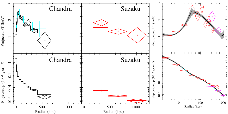
Figure 5.— Radial temperature (top panels) and density (bottom panels) profiles for RXJ 1159+5531. We show the projected Chandra profiles in the left column (triangles), the projected Suzaku profiles in the right column (stars), and the deprojected profiles in the right column. Overlaid are the best hydrostatic model fits to each dataset, which match the data very well and, for the deprojected profiles, we show in grey the 1-$\sigma$ confidence region for the model. We exclude the central Suzaku bin from the fitting (although it was used for abundance determination) since two temperature components were required, to account for the strong temperature gradient. In the upper left panel, we show the projected temperature profile measured by Vikhlinin et al. (2006) from the Chandra data (light blue crosses), which agrees well with our data. In the bottom right panel, we show (light blue dashed line) the deprojected density profile found by Vikhlinin et al. (2006), which is also in reasonable agreement with our data.

The projected gas temperature and density profiles are shown in Fig 5 for Chandra and Suzaku. These profiles span almost 3 orders of magnitude in radius. The outermost Suzaku data-bin reaches $\sim$1200 kpc, which is $\sim$${\rm R_{vir}}$, as found by Gastaldello et al. (2007b); see also § 4.2. There is excellent agreement between the results for the two satellites, giving us confidence in our treatment of the mixing between Suzaku annuli, and our treatment of the background components, which differ slightly between both satellites. Since two APEC components were employed in the central Suzaku bin, we do not show the gas density or temperature for that bin. The Chandra temperature profile agrees well with that found by Vikhlinin et al. (2006). In Fig 5, we also show the deprojected temperature profile (see § 6.4 for a description of how this was obtained), which is in good agreement with the deprojected profile reported for the Chandra data by Gastaldello et al. (2007b).

As discussed in § 3.1, there is evidence that the gas temperature may continue to fall in the central bin, possibly requiring a second APEC component to be added to the spectrum in this region. Nevertheless, the results for the single temperature fit can still be interpreted in our mass-fitting analysis, provided care is taken to compute an appropriately weighted average gas density and temperature in that region (see H11 for more details). In any case, we found that our results were relatively insensitive to the inclusion or omission of that particular annulus (§ 6.6).

4. Mass modelling

4.1. Method

We translated the density and temperature profiles into mass constraints using the entropy-based “forward-fitting” technique developed in our recent papers (Humphrey et al. 2008, 2009a; H11; Buote & Humphrey 2011a, for a review). Briefly, given parametrized profiles of “entropy” (S=kT$n_{e}^{-2/3}$, where $n_{e}$ is the electron density) and gravitating mass (excluding the gas mass, which is computed self-consistently), plus the gas density at some canonical radius (for which we used 10 kpc), the three-dimensional temperature and density profiles can be calculated, under the hydrostatic equilibrium approximation and fitted to the data. This model assumes spherical symmetry, which is a standard assumption in X-ray hydrostatic modelling, even when the X-ray isophotes are not perfectly round, since deviations from sphericity likely only contribute a very small error ($\sim$few percent) into the recovered mass profile and baryon fraction (Buote & Humphrey 2011b; see also Piffaretti et al. 2003; Gavazzi 2005).

For the gravitating mass model, we assumed an NFW (Navarro et al., 1997) dark matter halo, the virial mass and concentration of which were free fit parameters, plus a model for the stellar mass. Since the projected stellar light of the central galaxy is known to be well-fitted by a de Vaucouleurs model (Vikhlinin et al., 1999), for the stellar mass component, we adopted a deprojected de Vaucouleurs model, using the analytical approximation of Prugniel & Simien (1997). We fixed the effective radius and luminosity of this component to the K-band values (9.8 kpc, and $1.0\times 10^{12}$${\rm L_{\odot}}$ at the distance to RXJ 1159+5531), inferred from 2MASS (Gastaldello et al., 2007b), and allowed the K-band M/L ratio to be fitted freely. We additionally included a supermassive black hole, with mass fixed at $2.4\times 10^{9}$${\rm M_{\odot}}$, based on the ${\rm L_{K}}$ of the galaxy and the black-hole mass versus V-band bulge luminosity relation of (Gultekin et al., 2009), assuming $L_{V}/L_{K}=0.24$, which is typical for an old stellar population with Solar abundances.

To fit the three-dimensional entropy profile we assumed a model comprising a broken powerlaw, plus a constant; such a model is reasonably successful at reproducing the entropy profiles of galaxies and galaxy groups over a wide radial range (Humphrey et al., 2009a; Jetha et al., 2007; Finoguenov et al., 2007; Gastaldello et al., 2007a; Sun et al., 2009). In order to provide more flexibility in fitting the data (and weight more heavily the outer data-points in the fit), we also allow an additional break in the entropy profile at large radius. The normalization of the powerlaw and constant components, the radius of the breaks and the slopes above and below them were allowed to fit freely.

Following Humphrey et al. (2008), we solved the equation of hydrostatic equilibrium to determine the gas properties as a function of radius, from 10 pc to a large radius outside the field of view. For the latter, we adopted twice the virial radius of the system defined by ignoring the baryonic components (which is slightly smaller than the true virial radius of the system), but explore alternative choices in § 6.4. For any arbitrary set of mass and entropy model parameters, it is not always possible to find a physical solution to this equation over the full radial range. Such models were therefore rejected as unphysical during parameter space exploration. In order to compare to the observed projected density and temperature profiles, we projected the three-dimensional gas density and temperature, using a procedure similar to that described in Gastaldello et al. (2007b). This involves computing an emission-weighted projected mean temperature and density in each radial bin, that can be compared directly to the data.

To compare the model to the data, we used the $\chi^{2}$ statistic, fitting simultaneously the Chandra and Suzaku temperature and density profiles, with the central bin of the Suzaku data excluded from our fits. Correlations between the density errors were simply implemented by adopting a form for the $\chi^{2}$ statistic which incorporates the covariance matrix (e.g. Gould, 2003). Parameter space was explored with a Bayesian Monte Carlo method. Specifically, we used version 2.7 of the MultiNest code (Feroz & Hobson, 2008; Feroz et al., 2009). Since the choice of priors is nontrivial, we followed convention in cycling through a selection of different priors and assessing their impact on our results (we discuss this in detail in § 6.5). Initially, however, we adopted flat priors on the logarithm of the dark matter mass (over the range $10^{12}<M<10^{16}$${\rm M_{\odot}}$), the logarithm of the dark matter halo concentration, $c_{DM}$ (over the range $1<c_{DM}<100$), the logarithm of the gas density at the canonical radius, the stellar M/${\rm L_{K}}$ ratio, and the various entropy parameters. For a more detailed description of the modelling procedure, see Humphrey et al. (2009a); Buote & Humphrey (2011a).

4.2. Mass profile

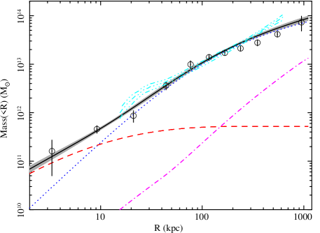
Figure 6.— Radial mass profile of RXJ 1159+5531. The solid (black) line indicates the total enclosed mass (and the grey shaded region indicates the 1-$\sigma$ error in the total mass distribution), the dashed (red) line indicates the stellar mass, the dotted (blue) line is the dark matter, and the dash-dot (magenta) line is the gas mass contribution. Overlaid are a set of data-points derived from a more traditional analysis method described in Humphrey et al. (2009a). We stress that the model is not fitted to these data, but is derived independently from the temperature and density data; nevertheless, the agreement between the different approaches is good. We also show the mass profile found by Vikhlinin et al. (2006) from the Chandra data (light blue dash-dot-dot line), which overall agrees with our results, although is higher at both large and small radii.

Table 1Mass results and error budget

Test	M∗/${\rm L_{K}}$	log ${\rm M_{2500}}$	log $c_{2500}$	log ${\rm M_{500}}$	log $c_{500}$	log ${\rm M_{vir}}$	log ${\rm c_{vir}}$
	${\rm M_{\odot}}$${\rm L_{\odot}}$-1	[${\rm M_{\odot}}$]		[${\rm M_{\odot}}$]		[${\rm M_{\odot}}$]
Marginalized	$0.54\pm 0.10$	$13.49^{+0.03}_{-0.02}$	$0.44\pm 0.07$	$13.77\pm 0.04$	$0.76\pm 0.06$	$13.97^{+0.05}_{-0.04}$	$1.05\pm 0.06$
Best-fit	$(0.51)$	$(13.49)$	$(0.48)$	$(13.75)$	$(0.80)$	$(13.95)$	$(1.09)$
$\Delta$DM profile	$+0.19$ $\left({}^{+0.08}_{-0.11}\right)$	$-0.024$ $\left({}^{+0.02}_{-0.03}\right)$	…	$+0.06$ $\left({}^{+0.02}_{-0.03}\right)$	…	$+0.21$ $\left(\pm{0.02}\right)$	…
$\Delta$AC	$-0.209$ $\left({}^{+0.10}_{-0.06}\right)$	$+0.003$ $\left(\pm{0.03}\right)$	$-0.015$ $\left({}^{+0.07}_{-0.08}\right)$	$+0.008$ $\left(\pm{0.04}\right)$	$-0.013$ $\left({}^{+0.06}_{-0.08}\right)$	$+0.02$ $\left({}^{+0.04}_{-0.05}\right)$	$-0.017$ $\left(\pm{0.07}\right)$
$\Delta$Background	${}^{+0.02}_{-0.06}$ $\left({}^{+0.10}_{-0.13}\right)$	${}^{+0.01}_{-0.02}$ $\left(\pm{0.03}\right)$	${}^{+0.02}_{-0.01}$ $\left(\pm{0.07}\right)$	${}^{+0.01}_{-0.03}$ $\left(\pm{0.04}\right)$	${}^{+0.02}_{-0.01}$ $\left(\pm{0.07}\right)$	${}^{+0.02}_{-0.02}$ $\left(\pm{0.04}\right)$	${}^{+0.03}_{-0.01}$ $\left(\pm{0.07}\right)$
$\Delta$SWCX	$-0.193$ $\left({}^{+0.11}_{-0.14}\right)$	$-0.027$ $\left(\pm{0.04}\right)$	$+0.10$ $\left({}^{+0.07}_{-0.09}\right)$	$-0.052$ $\left(\pm{0.05}\right)$	$+0.09$ $\left({}^{+0.06}_{-0.08}\right)$	$-0.047$ $\left(\pm{0.05}\right)$	$+0.09$ $\left({}^{+0.06}_{-0.08}\right)$
$\Delta$Stray light	$-0.005$ $\left(\pm{0.10}\right)$	$+0.01$ $\left({}^{+0.02}_{-0.03}\right)$	$-0.006$ $\left(\pm{0.07}\right)$	$+0.003$ $\left(\pm{0.04}\right)$	$-0.006$ $\left(\pm{0.06}\right)$	$+0.006$ $\left(\pm{0.04}\right)$	$-0.007$ $\left(\pm{0.06}\right)$
$\Delta$Rmax	${}^{+0.02}_{-0.01}$ $\left(\pm{0.10}\right)$	${}^{+0.01}_{-0.00}$ $\left(\pm{0.03}\right)$	${}^{+0.01}_{-0.00}$ $\left(\pm{0.07}\right)$	$-0.018$ $\left({}^{+0.05}_{-0.03}\right)$	$\pm 0.01$ $\left(\pm{0.06}\right)$	$\pm 0.01$ $\left(\pm{0.04}\right)$	$\pm 0.01$ $\left(\pm{0.06}\right)$
$\Delta$3d	$+0.05$ $\left(\pm{0.09}\right)$	$-0.049$ $\left(\pm{0.04}\right)$	$+0.02$ $\left(\pm{0.08}\right)$	$-0.053$ $\left(\pm{0.05}\right)$	$+0.02$ $\left(\pm{0.07}\right)$	$-0.040$ $\left(\pm{0.05}\right)$	$+0.02$ $\left(\pm{0.07}\right)$
$\Delta$Fit priors	${}^{+0.03}_{-0.01}$ $\left(\pm{0.11}\right)$	$+0.01$ $\left(\pm{0.03}\right)$	${}^{+0.01}_{-0.03}$ $\left(\pm{0.08}\right)$	$\pm 0.01$ $\left(\pm{0.04}\right)$	${}^{+0.01}_{-0.03}$ $\left(\pm{0.07}\right)$	${}^{+0.02}_{-0.00}$ $\left(\pm{0.05}\right)$	${}^{+0.01}_{-0.03}$ $\left(\pm{0.07}\right)$
$\Delta$Stars	$-0.031$ $\left({}^{+0.00}_{0.00}\right)$	$\pm 0$ $\left({}^{+0.02}_{-0.03}\right)$	$+0.08$ $\left(\pm{0.10}\right)$	$-0.020$ $\left({}^{+0.03}_{-0.05}\right)$	$+0.07$ $\left(\pm{0.09}\right)$	$-0.022$ $\left({}^{+0.04}_{-0.06}\right)$	$+0.05$ $\left({}^{+0.10}_{-0.07}\right)$
$\Delta$Weighting	$+0.09$ $\left({}^{+0.06}_{-0.09}\right)$	$+0.03$ $\left(\pm{0.03}\right)$	$-0.082$ $\left(\pm{0.07}\right)$	$+0.04$ $\left(\pm{0.04}\right)$	$-0.074$ $\left(\pm{0.06}\right)$	$+0.05$ $\left(\pm{0.04}\right)$	$-0.069$ $\left(\pm{0.06}\right)$
$\Delta$PSF	$\pm 0.01$ $\left(\pm{0.11}\right)$	$+0.01$ $\left({}^{+0.02}_{-0.03}\right)$	$-0.012$ $\left(\pm{0.07}\right)$	$+0.01$ $\left(\pm{0.05}\right)$	$-0.011$ $\left(\pm{0.06}\right)$	$+0.02$ $\left(\pm{0.05}\right)$	$-0.012$ $\left(\pm{0.06}\right)$
$\Delta$Instrument	${}^{+0.02}_{-0.03}$ $\left(\pm{0.11}\right)$	$+0.03$ $\left(\pm{0.03}\right)$	${}^{+0.02}_{-0.05}$ $\left(\pm{0.08}\right)$	${}^{+0.04}_{-0.01}$ $\left(\pm{0.05}\right)$	${}^{+0.02}_{-0.05}$ $\left(\pm{0.07}\right)$	${}^{+0.04}_{-0.01}$ $\left(\pm{0.05}\right)$	${}^{+0.02}_{-0.05}$ $\left(\pm{0.07}\right)$
$\Delta$Spectral	$+0.05$ $\left(\pm{0.10}\right)$	$+0.03$ $\left({}^{+0.02}_{-0.03}\right)$	$-0.019$ $\left(\pm{0.07}\right)$	$+0.02$ $\left(\pm{0.04}\right)$	$-0.018$ $\left(\pm{0.06}\right)$	$+0.02$ $\left(\pm{0.04}\right)$	$-0.016$ $\left(\pm{0.06}\right)$
$\Delta$Distance	${}^{+0.15}_{-0.12}$ $\left(\pm{0.13}\right)$	${}^{+0.01}_{-0.03}$ $\left({}^{+0.04}_{-0.02}\right)$	$\pm 0.11$ $\left(\pm{0.07}\right)$	${}^{+0.03}_{-0.08}$ $\left({}^{+0.05}_{-0.03}\right)$	$\pm 0.10$ $\left(\pm{0.07}\right)$	${}^{+0.07}_{-0.08}$ $\left(\pm{0.04}\right)$	$\pm 0.09$ $\left(\pm{0.06}\right)$
$\Delta$Entropy	$+0.01$ $\left({}^{+0.08}_{-0.12}\right)$	$+0.005$ $\left(\pm{0.03}\right)$	$-0.007$ $\left(\pm{0.07}\right)$	$-0.003$ $\left(\pm{0.04}\right)$	$-0.007$ $\left(\pm{0.06}\right)$	$+0.006$ $\left(\pm{0.04}\right)$	$-0.006$ $\left(\pm{0.06}\right)$
$\Delta$Covariance	${}^{+0.02}_{-0.03}$ $\left({}^{+0.08}_{-0.15}\right)$	${}^{+0.00}_{-0.01}$ $\left(\pm{0.03}\right)$	$+0.04$ $\left({}^{+0.06}_{-0.08}\right)$	$-0.028$ $\left(\pm{0.04}\right)$	$+0.03$ $\left({}^{+0.06}_{-0.08}\right)$	$-0.017$ $\left(\pm{0.04}\right)$	$+0.03$ $\left(\pm{0.06}\right)$

Note. — Marginalized values and 1-$\sigma$ confidence regions for the stellar mass-to-light (M_∗/${\rm L_{K}}$) ratio and the enclosed mass and concentration measured at various overdensities. Since the best-fitting parameters need not be identical to the marginalized values, we also list the best-fitting values for each parameter (in parentheses). In addition to the statistical errors, we also show estimates of the error budget from possible sources of systematic uncertainty. We consider a range of different systematic effects, which are described in detail in § 6; specifically we evaluate the effect of the choice of dark matter halo model ($\Delta$DM), adiabatic contraction ($\Delta$AC), treatment of the background ($\Delta$Background) and the Solar wind charge exchange X-ray component ($\Delta$SWCX), stray light ($\Delta$Stray light) maximum radius used in the projection calculation (${\rm\Delta R_{max}}$), deprojection ($\Delta$3d), priors on the model parameters ($\Delta$Fit priors), treatment of the stellar light ($\Delta$Stars), removing the emissivity correction ($\Delta$Weighting), the effect of errors in our treatment of spectral mixing due to the PSF of Suzaku ($\Delta$PSF), the X-ray detectors used ($\Delta$Instrument), spectral fitting choices ($\Delta$Spectral), distance uncertainties ($\Delta$Distance), the parameterization of the entropy model ($\Delta$Entropy), and covariance between the temperature and density data-points ($\Delta$Covariance). We list the change in the marginalized value of each parameter for every test and, in parentheses, the statistical uncertainty on the parameter determined from the test. Note that the systematic error estimates should not in general be added in quadrature with the statistical error.

We found the model could fit the density and temperature data well, with a best-fitting $\chi^{2}$/dof=14.4/15, even when taking into account the covariance between adjacent density data-points (see H11). The best-fitting models are overlaid in Fig 5. In Fig 5, we also show the range of possible three-dimensional temperature and density profiles predicted by our model that are consistent with the projected data. In Table 1, we tabulate the best-fitting values and marginalized confidence regions for each mass parameter of interest. The best-fitting radial mass distribution is shown in Fig 6, along with the relative contributions of each of the different mass model components. Overlaid are a series of mass data points derived from fitting the deprojected data using the “traditional smoothed inversion” mass modelling method (Buote & Humphrey, 2011a), which is more subject to systematic uncertainties (for more details see § 6.4 and Humphrey et al., 2009a). The agreement is very good, indicating that the resulting mass profile is not overly sensitive to the analysis method.

We obtain a marginalized ${\rm R_{vir}}$=$1100\pm 31$ kpc, which compares to an outer Suzaku annulus spanning 820–1190 kpc (thus having an “effective centre” at $\sim$1000 kpc). Therefore, we confirm that we are able to reach ${\rm R_{vir}}$ with these data.

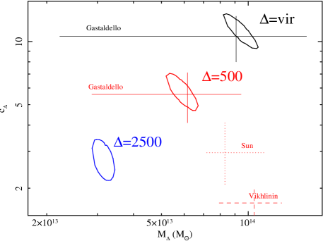
Figure 7.— Derived relation between mass and concentration for RXJ 1159+5531 (contours). We show the results for several over-densities (virial$\equiv$108, in black; 500 in red; 2500 in blue). We also compare our results to constraints reported in the literature (Gastaldello et al., 2007b; Vikhlinin et al., 2006; Sun et al., 2009).

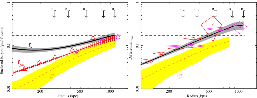
Figure 8.— Left: Radial distribution of the enclosed gas fraction (${\rm f_{gas}}$) and baryon fraction (${\rm f_{b}}$) in RXJ 1159+5531. The blue dotted line indicates the Univeral baryon fraction (0.17: Dunkley et al., 2009; Komatsu et al., 2011), while we also indicate various interesting radii. In yellow, we show the predicted ${\rm f_{gas}}$ profile at this mass scale from recent numerical simulations (Young et al., 2011). Right: The local (differential) gas fraction profile. At large radii, this exceeds the Universal value, indicating that gas has been pushed out to these scales.

In Fig 7, we show the relation between the concentration of the gravitating mass, ${\rm c_{vir}}$, and the virial mass, ${\rm M_{vir}}$. To be consistent with our past work (Buote et al., 2007), the ${\rm M_{vir}}$ and ${\rm R_{vir}}$ are derived from the distribution of the total gravitating mass, not just the dark matter, and the concentration, ${\rm c_{vir}}$ is defined as the ratio of ${\rm R_{vir}}$ to the characteristic scale of the DM halo. We compare our results with concentration and mass constraints for RXJ 1159+5531 reported in the literature (and based only on the Chandra data) at different overdensities. We find excellent agreement with the ${\rm M_{vir}}$-${\rm c_{vir}}$ results from Gastaldello et al. (2007b); in particular the agreement with the virial mass and concentration obtained from that paper is interesting, given that the Gastaldello et al. (2007b) results at this overdensity were significantly extrapolated. We do, however, find a systematic offset at ${\rm R_{500}}$ from the work of Sun et al. (2009) and Vikhlinin et al. (2006), who employed essentially the same “smoothed inversion” mass modelling approach (Buote & Humphrey, 2011a) in each work, and obtained slightly higher masses and lower concentrations than our best-fitting values. We discuss the possible origin of these discrepancies in § 7.2.

Table 2Baryon fraction results and error budget

Test	$f_{g,2500}$	$f_{g,500}$	$f_{g,vir}$	$f_{b,2500}$	$f_{b,500}$	$f_{b,vir}$
Marginalized	$0.048\pm 0.001$	$0.087\pm 0.005$	$0.14\pm 0.02$	$0.12^{+0.009}_{-0.01}$	$0.124^{+0.007}_{-0.008}$	$0.17\pm 0.02$
Best-fit	$(0.048)$	$(0.089)$	$(0.149)$	$(0.117)$	$(0.127)$	$(0.174)$
$\Delta$DM profile	$+0.002$ $\left(\pm{0.001}\right)$	$-0.005$ $\left(\pm{0.004}\right)$	$-0.044$ $\left(\pm{0.01}\right)$	$+0.03$ $\left(\pm{0.01}\right)$	$\pm 0$ $\left({}^{+0.006}_{-0.008}\right)$	$-0.046$ $\left(\pm{0.01}\right)$
$\Delta$AC	$\pm 0$ $\left({}^{+0.002}_{-0.001}\right)$	$\pm 0$ $\left(\pm{0.005}\right)$	$-0.003$ $\left(\pm{0.02}\right)$	$-0.022$ $\left(\pm{0.01}\right)$	$-0.012$ $\left({}^{+0.006}_{-0.007}\right)$	$-0.009$ $\left(\pm{0.02}\right)$
$\Delta$Background	$+0.001$ $\left(\pm{0.001}\right)$	${}^{+0.004}_{-0.001}$ $\left(\pm{0.006}\right)$	${}^{+0.02}_{-0.01}$ $\left(\pm{0.02}\right)$	${}^{+0.00}_{-0.00}$ $\left(\pm{0.01}\right)$	$\pm 0.00$ $\left(\pm{0.01}\right)$	${}^{+0.02}_{-0.01}$ $\left(\pm{0.02}\right)$
$\Delta$SWCX	$+0.001$ $\left({}^{+0.001}_{-0.002}\right)$	$+0.003$ $\left(\pm{0.005}\right)$	$+0.02$ $\left({}^{+0.01}_{-0.02}\right)$	$-0.021$ $\left({}^{+0.02}_{-0.01}\right)$	$-0.005$ $\left({}^{+0.01}_{-0.01}\right)$	$+0.02$ $\left({}^{+0.01}_{-0.02}\right)$
$\Delta$Stray light	$\pm 0$ $\left(\pm{0.001}\right)$	$-0.002$ $\left(\pm{0.005}\right)$	$-0.007$ $\left(\pm{0.02}\right)$	$-0.003$ $\left(\pm{0.01}\right)$	$-0.003$ $\left(\pm{0.01}\right)$	$-0.005$ $\left(\pm{0.02}\right)$
$\Delta$Rmax	$\pm 0$ $\left(\pm{0.001}\right)$	$+0.002$ $\left({}^{+0.005}_{-0.006}\right)$	$+0.004$ $\left(\pm{0.02}\right)$	$-0.001$ $\left(\pm{0.01}\right)$	$-0.001$ $\left(\pm{0.01}\right)$	$+0.009$ $\left({}^{+0.01}_{-0.02}\right)$
$\Delta$3d	$+0.004$ $\left(\pm{0.002}\right)$	$+0.01$ $\left({}^{+0.007}_{-0.005}\right)$	$+0.03$ $\left(\pm{0.02}\right)$	$+0.02$ $\left(\pm{0.01}\right)$	$+0.02$ $\left({}^{+0.01}_{-0.01}\right)$	$+0.04$ $\left(\pm{0.02}\right)$
$\Delta$Fit priors	$\pm 0$ $\left(\pm{0.002}\right)$	$-0.002$ $\left(\pm{0.005}\right)$	${}^{+0.003}_{-0.005}$ $\left(\pm{0.02}\right)$	${}^{+0.00}_{-0.00}$ $\left(\pm{0.01}\right)$	${}^{+0.00}_{-0.00}$ $\left(\pm{0.01}\right)$	${}^{+0.00}_{-0.00}$ $\left(\pm{0.02}\right)$
$\Delta$Stars	$\pm 0$ $\left({}^{+0.001}_{-0.001}\right)$	$+0.002$ $\left(\pm{0.005}\right)$	$+0.009$ $\left(\pm{0.02}\right)$	${}^{+0.03}_{-0.04}$ $\left(\pm{0.01}\right)$	$\pm 0.02$ $\left(\pm{0.01}\right)$	$\pm 0.01$ $\left(\pm{0.02}\right)$
$\Delta$Weighting	$\pm 0$ $\left({}^{+0.002}_{-0.001}\right)$	$-0.002$ $\left(\pm{0.005}\right)$	$-0.015$ $\left({}^{+0.01}_{-0.02}\right)$	$+0.003$ $\left(\pm{0.01}\right)$	$-0.003$ $\left(\pm{0.01}\right)$	$-0.016$ $\left(\pm{0.02}\right)$
$\Delta$PSF	$\pm 0$ $\left(\pm{0.002}\right)$	$-0.002$ $\left(\pm{0.005}\right)$	$-0.010$ $\left(\pm{0.02}\right)$	$-0.005$ $\left(\pm{0.01}\right)$	$-0.003$ $\left(\pm{0.01}\right)$	$-0.006$ $\left(\pm{0.02}\right)$
$\Delta$Instrument	$+0.002$ $\left({}^{+0.002}_{-0.002}\right)$	$-0.003$ $\left(\pm{0.01}\right)$	$-0.028$ $\left({}^{+0.02}_{-0.03}\right)$	$-0.006$ $\left(\pm{0.01}\right)$	$-0.005$ $\left(\pm{0.01}\right)$	$-0.026$ $\left({}^{+0.02}_{-0.03}\right)$
$\Delta$Spectral	$-0.003$ $\left(\pm{0.001}\right)$	$-0.007$ $\left(\pm{0.005}\right)$	$-0.020$ $\left(\pm{0.02}\right)$	$-0.004$ $\left(\pm{0.01}\right)$	${}^{+0.00}_{-0.01}$ $\left(\pm{0.01}\right)$	$-0.017$ $\left(\pm{0.02}\right)$
$\Delta$Distance	${}^{+0.01}_{-0.01}$ $\left(\pm{0.002}\right)$	${}^{+0.02}_{-0.01}$ $\left(\pm{0.01}\right)$	${}^{+0.03}_{-0.02}$ $\left(\pm{0.02}\right)$	$+0.003$ $\left(\pm{0.01}\right)$	${}^{+0.01}_{-0.00}$ $\left(\pm{0.01}\right)$	${}^{+0.02}_{-0.01}$ $\left(\pm{0.02}\right)$
$\Delta$Entropy	$\pm 0$ $\left(\pm{0.002}\right)$	$\pm 0$ $\left(\pm{0.005}\right)$	$-0.001$ $\left(\pm{0.02}\right)$	$-0.003$ $\left(\pm{0.01}\right)$	$\pm 0$ $\left(\pm{0.01}\right)$	$\pm 0$ $\left(\pm{0.02}\right)$
$\Delta$Covariance	$\pm 0$ $\left({}^{+0.002}_{-0.001}\right)$	$+0.004$ $\left({}^{+0.005}_{-0.006}\right)$	${}^{+0.011}_{-0.002}$ $\left(\pm{0.02}\right)$	$-0.002$ $\left({}^{+0.01}_{-0.01}\right)$	${}^{+0.00}_{-0.00}$ $\left(\pm{0.01}\right)$	$+0.01$ $\left(\pm{0.02}\right)$

Note. — Marginalized values and 1-$\sigma$ confidence regions for the gas fraction ($f_{g,\Delta}$) and baryon fraction ($f_{b,\Delta}$) measured at various overdensities ($\Delta$). We also provide the best-fitting parameters in parentheses, and a breakdown of possible sources of systematic uncertainty, following Table 1. We find that $f_{b}$ is reasonably robust to most sources of systematic uncertainty, especially within ${\rm R_{2500}}$.

4.3. Gas and baryon fraction constraints

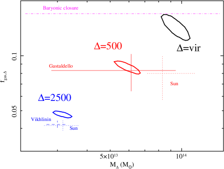
Figure 9.— Contours of ${\rm f_{gas}}$ versus mass at different over-densities. The magenta (dash-dot) line indicates the Universal baryon fraction (annotated “baryonic closure”). We overlay results from the literature.

In Table 2, we tabulate the best-fitting values and marginalized confidence regions for the gas and baryon fractions of the system at different overdensities. In performing this calculation, we included the mass in baryons of the central galaxy and the hot gas (inferred from our fit), and also folded in two additional, uncounted reservoirs of baryons, intra-cluster light and additional galaxies in the group. Vikhlinin et al. (1999) found that $\sim$25% of the V-band stellar light associated with galaxies was in non-central galaxies. We assumed that this also holds in the K-band, and adopted a K-band M/L ratio of 1 for these galaxies. Furthermore, for the virial mass of the system, we expect as much as $\sim$2 times the stellar mass of the central galaxy will be bound up in intra-cluster light (Purcell et al., 2007). If we make the reasonable assumption that these uncounted baryons are distributed in the same way as the dark matter (this is approximately true of the additional galaxy light reported by Vikhlinin et al.), the total mass inferred from our modelling (which did not explicitly include these components) will be correct. We discuss the sensitivity of our results to our treatment of these components in § 6.6. In practice, however, these uncounted components account for only $\sim$10% of the baryon budget, since most of the baryons are tied up in the hot gas halo.

In Fig 8, we display the radial dependence of enclosed baryon fraction, which rises modestly from ${\rm f_{b}}$$\sim$0.1 at 100 kpc to $0.17\pm 0.02$ by ${\rm R_{vir}}$, in excellent agreement with the Cosmological baryon fraction (0.17: Dunkley et al., 2009; Komatsu et al., 2011). We stress there is no extrapolation in this measurement of ${\rm f_{b}}$ at the virial radius, since the Suzaku data reach the virial radius in this system. This behaviour is strikingly similar to the isolated Galaxy NGC 720 (H11), which has a virial mass $\sim$2 orders of magnitude smaller than RXJ 1159+5531.

In Fig 8, we also show the radial distribution of the enclosed gas fraction, which rises steeply with radius (as is typically observed in groups and clusters, e.g. Vikhlinin et al. 2006). For comparison, we overlay the predictions of recent numerical simulations (Young et al., 2011), which systematically under-estimate the true gas fraction. At small scales (or higher overdensities) the low ${\rm f_{gas}}$ indicates that gas has either been bound up into stars or “pushed out” to large radii by feedback. However, the approximate baryonic closure of the system suggests that little gas has been evacuated completely from the system in such a process. That gas has been “pushed out” in this way is reflected in the differential gas fraction (i.e.the gas density divided by the total mass density at a given radius), which actually exceeds the Cosmological baryon fraction outside $\sim$500 kpc (Fig 8, right panel). In all, we find that $\sim$65% of the gas within ${\rm R_{vir}}$ actually lies outside ${\rm R_{500}}$, illustrating the importance of the Suzaku data for directly measuring it.

In Fig 9, we compare our enclosed ${\rm f_{gas}}$ constraints at different overdensities with values reported in the literature. Once again, our measurements agree well with Gastaldello et al. (2007b), but there are some modest discrepancies with Sun et al. (2009) and Vikhlinin et al. (2006), who found slightly smller ${\rm f_{gas}}$. We will discuss the possible origin of these differences in § 7.2.

4.4. Entropy profile

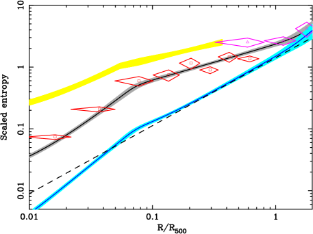
Figure 10.— Entropy profile model of RXJ 1159+5531, scaled by its characteristic entropy, and shown as a function of ${\rm R_{500}}$. The grey shaded region is the 1-$\sigma$ confidence region determined from our mass model fit. We overlay deprojected data-points from Chandra (triangles) and Suzaku (stars), which are determined more directly from the data, and agree well with the model. We stress the model is not fitted to these data. We note that the deprojection procedure in large spatial bins likely introduces non-neglible (unphysical) noise into the data-points (see § 6.4), and so they should be treated with caution. The dotted line indicates the “baseline” predictions from gravitational structure formation (Voit et al., 2005), and we find that the “${\rm f_{gas}}$-corrected” entropy profile (blue shaded region; see text), which agrees well with the baseline predictions out to $\sim$${\rm R_{vir}}$. Also shown (yellow region) is the scaled entropy profile of the isolated elliptical galaxy NGC 720, illustrating more entropy injection in the lower-mass system.

As expected for approximately hydrostatic gas, we find that we obtain a good fit to the data with a model requiring a monotonically rising entropy (S) profile. We show the model profile in Fig 10 (grey shaded region), scaled by the “characteristic entropy” ${K_{500}}$ (Voit et al., 2005), and shown as a function of fraction of ${\rm R_{500}}$ reached. In the inner part of the system, the slope ($S\sim R^{\beta}$) is slightly steeper than the canonical $\beta\sim$1.1, and the normalization is significantly enhanced over the “baseline” model for gravity-only structure formation simulations (Voit et al., 2005), indicating significant entropy injection. Above $\sim$40 kpc ($\sim$0.07${\rm R_{500}}$), the entropy profile flattens significantly, and converges with the (steeper) baseline model by ${\rm R_{vir}}$. For maximum flexibility, we allowed an additional break at large radii, but found that it was poorly constrained, and the overall shape of the distribution is very flat from $\sim$40 kpc to $\sim$${\rm R_{vir}}$; in fact, fits omitting the break are able to fit the data just as well, with only a minimal impact on the recovered gas properties (§ 6.9).

To provide a less model-dependent view of the entropy profile, we overlay in Fig 10 a series of data-points, which are directly computed from the deprojected density and temperature profiles. These were obtained by emulating the behaviour of the “projct” Xspec model, and correcting for emission projected into the line of sight from outside the outermost annulus (see H11). These data agree well with the smooth model, giving us confidence in our treatment of the data.

Following Pratt et al. (2010), we investigated the effect of scaling the entropy profile by a simple correction factor, $S_{corr}=S_{obs}(f_{g}/0.17)^{2/3}$, where $S_{corr}$ is the corrected entropy profile, and $S_{obs}$ is the observed (scaled) distribution. As for more massive galaxy clusters (Pratt et al.), and the isolated elliptical galaxy NGC 720 (H11), we find that $S_{corr}$ is in much better agreement with the baseline entropy model (Fig 10).

4.5. Rosat surface brightness profile

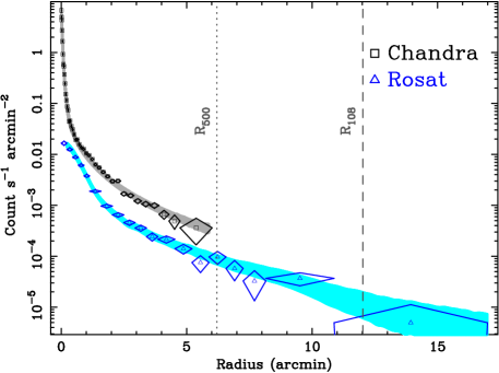
Figure 11.— Comparison of the flat-fielded, background-subtracted 0.3–7.0 keV Chandra (black squares) and 0.42–2 keV Rosat (blue triangles) surface brightness profiles for RXJ 1159+5531. Overlaid are the profiles predicted by the best-fitting model; the shaded regions correspond to the 1-$\sigma$ uncertainty. The vertical displacement between the Rosat and Chandra data reflects differences in the effective area curves and energy-bands. In practice, our model agrees very well with the Rosat data, out as far as $\sim$17′. The vertical lines indicate ${\rm R_{500}}$ and ${\rm R_{vir}}$.

We next explored whether the model fitted to the Chandra and Suzaku data are consistent with the Rosat surface brightness profile (e.g. Eckert et al., 2011). To do this, we computed the three-dimensional gas emissivity, based on our best-fitting models for the temperature, density and abundance profiles. This model was projected onto the sky and folded through the appropriate Rosat PSPC instrumental responses. To account for possible mis-calibration between the satellites, we allowed an arbitrary scaling of the model normalization between Chandra and Rosat. We broadened the surface brightness model by folding in the instrumental PSF, evaluated at 1 keV. We added a constant (sky) background component and allowed its normalization, and the aforementioned scaling factor, to fit to the Rosat surface brightness profile, using dedicated software based around the MINUIT fitting library. The best-fitting value of the scaling factor ($0.93\pm 0.03$) indicates good overall agreement, although there may be a modest calibration discrepancy, at least when observing a $\sim$1 keV source at large ($\sim$17′) off-axis angles with Rosat. Nevertheless, such a modest discrepancy will not affect our conclusions in the outer part of the group. The surface brightness profile was fitted out to $\sim$25′, and became consistent with the background outside $\sim$12′.

In Fig 11, we show the background-subtracted Rosat surface brightness profile (triangles) and, for comparison, the Chandra ACIS-S3 data. We overlay the predicted surface brightness models, illustrating excellent agreement with the Rosat data out beyond ${\rm R_{vir}}$. This strongly supports our treatment of the Suzaku (and Chandra) data, and confirms that the entropy profile does not exhibit substantial flattening outside $\sim$${\rm R_{500}}$.

5. The cosmic X-ray background

Figure 12.— Composite spectrum of the detected Chandra point-sources in the region of interest with fluxes $<2\times 10^{14}$${\rm erg\ s^{-1}\ cm^{-2}}$. The brightest few sources were omitted so that they do not unduly bias the fit. Overlaid is the canonical powerlaw ($\Gamma=1.41$) used to fit the CXB component, which gives a reasonably good overall fit to the data.

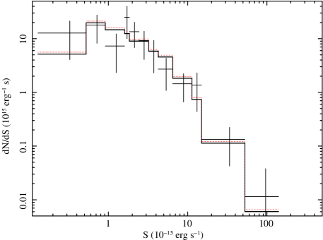
Figure 13.— The measured differential log N-log S relation for point-sources within the Chandra field of view. The down-turn at low fluxes is due to source detection incompleteness; we fold incompleteness and Eddington bias corrections into the fitted model. The dotted red line is the expected fit, based on the hard-source counts in Luo et al. (2008), and the solid black line is the CDF-S best-fitting model, rescaled to fit the data.

As is clear from Fig 2, the accurate determination of the gas properties in the outer two Suzaku annuli requires the background to be determined with high accuracy (see also § 6.2). The dominant background component of relevance is actually the cosmic X-ray background (CXB) resulting from (unrelated) undetected, background point-sources. In this section, we explore the accuracy with which the CXB component has been fitted in our Suzaku analysis.

Chandra’s spatial resolution allows a significant fraction of the CXB to be resolved into individual point sources, at least near the optical axis. By disentangling them from any diffuse emission, resolving the sources in this way allows the CXB spectral shape and normalization to be determined more precisely. Deep Chandra observations have yielded accurate measurements of the logN-logS distribution (and hence, average surface brightness) of background point sources along particular sightlines (e.g. Luo et al., 2008). Alternatively, X-ray spectra from regions of the sky free of foreground contamination have allowed the CXB shape and normalization to be carefully calibrated, averaged over small portions of the sky (e.g. De Luca & Molendi, 2004). However, due to cosmic variance and stochastic effects, the inferred surface brightness will not be well-enough known to use this information along other, arbitrary sightlines, such as that to RXJ 1159+5531. Ideally, therefore Chandra should be used to resolve the point-sources in each of the Suzaku annuli, and the resultant spectra can be used to refine the Suzaku analysis. Unfortunately, the more obstructed field of view of Chandra (at least in the ACIS-S configuration), coupled with the substantial degradation of the PSF (and hence, reduced detection efficiency) at $\mathrel{\hbox to0.0pt{\lower 3.0pt\hbox{$\sim$}\hss}\raise 2.0pt\hbox{$>$}}$ 4′ away from the optical axis, means that multiple Chandra observations are needed to mosaic the entirety of each Suzaku annulus at high enough precision. To complicate matters further, since point sources can be variable, contemporaneous observations with each satellite would ideally be used. Nevertheless, while individual sources can vary significantly, the integrated source properties are not expected to be strongly affected by variability (e.g. Kraft et al., 2001; Zezas et al., 2004).

Since the existing Chandra data did not meet these requirements, it was not possible to improve our Suzaku constraints using this approach. Nevertheless, it is still important to verify consistency between the Chandra and Suzaku CXB measurement. To do this, we first examined the sources detected by Chandra that lay within each Suzaku region. In the outermost region, we detected 9 sources, which we estimate (below) to contribute only $\sim$20% of the flux within this aperture. This estimate reflects both the fact that only $\sim$50% of this region is exposed with Chandra, and the large off-axis angles ($\sim$9-13′) under scrutiny. In the 2–5′ aperture, however, the Chandra data were more helpful; we estimate that $\sim$80% of the CXB flux was resolved into 26 detected sources. These estimates, of course, assume that the detected sources did not vary in brightness significantly between the Chandra and Suzaku observations.

In principle, one can sum the spectra of all detected sources within each region, and use that to determine the shape (if not the normalization) of the CXB spectrum. However, this estimate suffers from a bias, since it assumes that the spectrum of a background AGN is independent of its flux, which is not true. If we omitted sources above a particular flux limit from this calculation, the composite spectrum was systematically flatter. Fits to the CXB spectrum measured from unresolved background emission in source-free regions of the sky should not be affected by this problem, and so in our default analysis, we parameterized the CXB spectrum as a powerlaw with $\Gamma=1.41$, as found by De Luca & Molendi (2004). The incompleteness correction of the composite spectrum that is necessary to test formal consistency between this model and the Chandra data is beyond the scope of this paper. However, in Fig 12 we show the composite spectrum of sources fainter than $2\times 10^{-14}$${\rm erg\ s^{-1}\ cm^{-2}}$ (omitting the few, bright point sources in the field so as not to skew unfairly the spectral shape), which agrees reasonably well (if not perfectly) with this model. In § 6.2 we find that modest variation in the slope of the CXB component ($\pm$5%) does not strongly affect our conclusions.

While the CXB shape may vary modestly between sightlines, the uncertainty on its normalization is likely to be more problematical for our analysis. To verify consistency between the Suzaku flux in each aperture and the Chandra esimates requires an estimate not only of the mean flux, but also the uncertainty on it, from undetected sources in each region. To measure the mean flux, it was first necessary to determine the normalization and shape of the average logN-logS distribution for the point sources along the RXJ 1159+5531 line of sight. Since cosmic variance is unlikely to be strong between each Suzaku region, we considered all sources detected by Chandra that lay within the Suzaku XIS0 field of view. Following Humphrey & Buote (2008), we subtracted a local background from each source spectrum and converted the counts to 0.5–7.0 keV flux, assuming a powerlaw model ($\Gamma$=1.55) with Galactic absorption, while taking into account the spatial dependence of the effective area. Given the measured fluxes and spatial distribution, we do not believe any of these sources to be X-ray binaries associated with the central galaxy. The resulting logN-logS distribution (in $dN/dS$ form) is shown in Fig 13. In order to interpret these data, it was necessary to fit a model, correcting for both incompleteness at low fluxes and the Eddington bias. In Humphrey & Buote (2008), we discuss in detail how these corrections were carried out. In short, we corrected the model (not the data) based on the results of extensive Monte Carlo simulations in which fake sources were added (in a spatially uniform, random fashion) to the Chandra images, and the source detection algorithm was used to try to detect them and determine their flux.

We found that the $dN/dS$ distribution could be well-fitted with a (incompleteness-corrected) broken powerlaw model (with a break at $7.4\times 10^{-15}$${\rm erg\ s^{-1}\ cm^{-2}}$, and negative logarithmic differential slopes 1.3 and 2.6 below and above the break, respectively) that we also found could fit the hard-band logN-logS distribution reported by Luo et al. (2008) for the Chandra Deep Field South (CDF-S) line of sight. The best-fitting model is shown in Fig 13, which is very close to the fit to the CDF-S data (shown, correctly normalized for the observed region of sky). This good agreement gives us confidence in our treatment of the data.

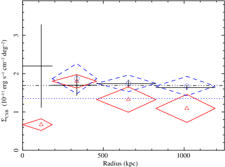
Figure 14.— The 0.5–7.0 keV surface brightness profile ($\Sigma_{CXB}$) of the CXB component, measured from the Suzaku, Rosat and Chandra data. We show the best-fitting $\Sigma_{CXB}$ from the default Suzaku analysis (black dash-dot-dot line), and $\Sigma_{CXB}$ determined independently from the Suzaku data in each region (black crosses). Also shown are the estimates from the Rosat surface brightness profile (dashed error bars; blue circles) and from fitting the Chandra point source distributions (red triangles). The blue dotted line is the expected flux from integrating the logN-logS point source distribution along the CDF-S line-of-sight (Luo et al., 2008, see text). We find excellent agreement between the different estimates. Note that the CXB component need not be constant with radius, and so we only expect good agreement only between the fitted data-points, not the approximate (constant) models shown.

While the average normalization of the CXB component along the RXJ 1159+5531 sightline can be determined in this way, the actual flux measured in any annulus is subject to stochastic scatter about this value due to the discrete source nature of the CXB. To account for this, we undertook Monte Carlo simulations, as outlined below:

1. Using the best-fitting logN-logS relation, described above, we determined the total number of sources per square degree, N₀ with flux $>10^{-16}$${\rm erg\ s^{-1}\ cm^{-2}}$. On each simulation, we added Gaussian noise to N₀ to reflect uncertainties ($\pm 12$%) in the fit to the logN-logS relation.

2. For each Suzaku region $i$, which has area $A_{i}$, we drew N_i sources that have fluxes distributed like the logN-logS relation between $10^{-16}$ and $10^{-12}$${\rm erg\ s^{-1}\ cm^{-2}}$. N_i was itself Poisson distributed around $N_{0}A_{i}$.

3. Based on the fraction of the Suzaku region covered by Chandra, and our source detection incompleteness estimates at each flux, every source has a particular probability of being detected. Using this information, we randomly assigned a state (detected, or not detected) to each source.

4. In each region $i$, we estimated the CXB flux by summing up the flux of all simulated sources flagged as “undetected”, and added in the flux of the real detected sources and the expected flux of sources below $10^{-16}$${\rm erg\ s^{-1}\ cm^{-2}}$ (by integrating the logN-logS relation).

5. We repeated steps 1–4 a large number of times to determine the average CXB flux and its uncertainty in each region $i$. This estimate accounts for both stochastic scatter and the uncertainty on the logN-logS normalization from our fit.

In Fig 14, we show the estimated X-ray flux for each bin. along with the value measured from the Suzaku spectral fitting. We show both the best-fitting value for our default analysis (in which the CXB normalization per square degree is tied between all the annuli), and the constraints on the CXB flux when the the normalization is allowed to fit freely in each region. The Chandra results appear to be in good agreement with the Suzaku measurements. If the integrated flux is very sensitive to the properties of individual, bright point sources, we would expect the CXB surface brightness measured by Suzaku to show significant scatter between each radial bin, in excess of the measured statistical error. In fact, the CXB surface brightness is consistent with being constant with radius.

As a final consistency check, we also explored whether the Rosat data agreed with the Suzaku results. We extracted the Rosat radial surface brightness profile in the band 1–2 keV; based on the best-fitting Suzaku background model, we expect that $\sim$95% of the background emission in this region comes from the unresolved CXB. We restricted the photons to be from the region of sky imaged by XIS0 (although we also excluded a 3.4′-wide region in the vicinity of the inner support ring shadow). We subtracted off the particle background, the expected (small) contribution from the soft Galactic background components (which was assumed to be spatially uniform), and the surface brightness profile predicted from our best fitting mass model (see § 4.5). The remaining counts should come from the CXB emission. Rebinning the profile to match the Suzaku annuli, and converting counts to flux by folding the canonical CXB model through the Rosat response matrices (computed close to the centre of RXJ 1159+5531), we obtained an estimate of the CXB surface brightness in excellent agreement with the Suzaku measurements (Fig 14).

6. Systematic error budget

In this section, we address the sensitivity of our results to various data analysis choices that were made. In most cases, it is difficult or impractical to express these assumptions through a single additional model parameter over which one might hope to marginalize, and so we adopted the pragmatic approach of investigating how our results changed if the assumptions were arbitrarily adjusted. We focused on those systematic effects likely to have the greatest impact on our conclusions, and list in Tables 1 and 2 the change to the marginalized value of each key parameter for each test. We outline below how each test was performed.

6.1. Dark Matter profile

One of the major sources of uncertainty on the recovered mass model is the coice of DM mass model. While the NFW model is theoretically motivated, we also experiemented with the so-called “cored logarithmic” mass model (Binney & Tremaine, 2008). This model tends to predict higher masses (by $\sim$60%), and correspondingly smaller gas fractions, at large scales. Although we cannot distinguish between the NFW and cored logarithmic models on the basis of $\chi^{2}$ alone, the ratio of the Bayesian evidence ($2.6\times 10^{-3}$) implies that the cored logarithmic model, with the adopted priors (a flat prior on the asymptotic circular velocity, between 10 and 2000 $km\ s^{-1}$, and a flat prior on $log_{10}r_{c}$, where $r_{c}$ is the core radius, over the range $0\leq log_{10}r_{c}\leq 3$.) is a poorer description of the data at $\sim$3.0-$\sigma$.

Another modification to the DM halo profile that is well-motivated theoretically, although less secure observationally (Humphrey et al., 2006; Gnedin et al., 2007; Napolitano et al., 2010), is so-called “adiabatic contraction” (Blumenthal et al., 1986; Gnedin et al., 2004; Abadi et al., 2009), where the DM halo density profile reacts to the gravitational influence of baryons that are condensing into stars by becoming cuspier. Modifying the NFW profile with the algorithm of Gnedin et al. (2004), has only a very slight effect on the best-fitting mass model (“$\Delta$AC” in Tables 1 and 2). This reflects that the scale radius of the DM halo is much larger than the effective radius of the stellar mass component.

6.2. Background

Since the data were background-dominated in the outermost Suzaku annuli, the treatment of the background was a potentially serious source of systematic uncertainty. To investigate the extent to which our results are sensitive to this, we explored a range of different choices. First, for the Chandra data, we adopted the standard blank-field events files distributed with the CALDB to extract a background spectrum for each annulus. Since the blank-field files for each CCD have different exposures, spectra were accumulated for each CCD individually, scaled to a common exposure time and then added. The spectra were renormalized to match the observed count-rate in the 9–12 keV band. These “template” spectra were then used as a background in Xspec, and the background model components were omitted from our fit. This gave a formally poorer fit, but did not strongly affect our conclusions. Second, since the Suzaku non X-ray background spectra generated by xisnxbgen may be uncertain, we allowed their normalization to scale by $\pm$5%.

At the temperature of the gas in the outermost annuli ($\sim$1 keV), the dominant background component is the CXB. In § 5, we demonstrated that the best-fitting CXB model to our data is in excellent agreement with predictions for the line of sight to RXJ 1159+5531. However, there were still uncertainties in our treatment. Specifically, by default, we assumed a constant surface brightness for the CXB component, which may not be formally correct. We therefore experimented with allowing the CXB normalization to fit freely in each Suzaku annulus (Fig 14). This did not significantly affect our results. Additionally, there is uncertainty on the spectral shape of the CXB component. Given the statistical uncertainty on the shape of the CXB parameterization found by De Luca & Molendi (2004), we varied the slope of the CXB powerlaw component by $\pm 5$%. Although this affected the error on the gas density at the largest radii, our conclusions were not significantly altered. Allowing a larger change in the slope did have a more significant effect on the density and temperature, however, motivating the need for deep Chandra data to resolve and constrain the CXB at the largest scales (§ 7.6). We summarize the results in Tables 1 and 2 (“$\Delta$Background”).

6.2.1 Solar Wind Charge Exchange

An additional background component can arise from the interaction of the Solar wind with interstellar material and the Earth’s exosphere. This should manifest itself as a time-variable, soft component that can be modelled as a series of narrow Gaussian lines, the intensity of which correlate with the Solar wind activity (e.g. Snowden et al., 2004). We did not explicitly include components to account for this “Solar Wind Charge Exchange” (SWCX) in our fits, although the soft background components are partially degenerate with it. To explore whether the SWCX could have affected our conclusions, we used the Solar Wind Ion Composition Spectrometer (SWICS) instrument aboard the Advanced Composition Explorer (ACE) spacecraft (McComas et al., 1998) to identify periods of enhanced SWCX emission. Following Snowden et al. (2004), we assumed it to be negligible when the ${\rm O^{+7}/O^{+6}}$ ratio falls below $\sim$0.2, and selected times during each observation which met this criterion. While the Chandra data were moderately affected ($\sim$60% of the data were excluded by this cut), in the low surface brightness regime, the Suzaku data were most important, and these were only mildly affected ($\sim$9% of the data were removed by this cut; the 0.5–1.0 keV count-rate was enhanced only by $\sim$6% if all the data were used). The corrected Chandra and Suzaku spectra were fitted to obtain the temperature and density profiles, and folded through our mass modelling apparatus. We found that our results were not substantially affected by correcting for the SWCX component (“$\Delta$SWCX” in Tables 1 and 2).

6.3. Stray light

Stray light from bright point sources within $\sim 1^{\circ}$ can, in principle, be scattered by the mirrors into the field of view, and provide an additional source of background. By far the brightest point source identified by the Rosat All-Sky Survey (RASS) within this angular distance from RXJ 1159+5531 is is NGC 3998, a foreground Sy1 galaxy which is 17′ from RXJ 1159+5531. To investigate the potential impact of stray light, we included an additional component in our spectral modelling, corresponding to the contamination from NGC 3998 to each annulus. We estimated the amount of stray light leakage by using xissimarfgen to generate suitable ancillary response files for each annulus, with the locus of NGC 3998 as the origin for the photons. We modelled the emission from NGC 3998 as an absorbed powerlaw, with $N_{H}$, $\Gamma$ and the normalization fixed to the values derived from archival XMM-Newton data by Ptak et al. (2004). We found that the stray light contamination was $<20$% of the source flux below $\mathrel{\hbox to0.0pt{\lower 3.0pt\hbox{$\sim$}\hss}\raise 2.0pt\hbox{$<$}}$ 2 keV. The stray light component is much harder than the $\sim$1 keV spectrum of the hot gas, and is partially degenerate with the CXB spectral component. Therefore, we found that adding this component had minimal effect on our results (“$\Delta$Stray light” in Tables 1 and 2).

6.4. Projection/ Deprojection

In our analysis, we modelled the projected temperature and density in each annulus by evaluating the hydrostatic model for the temperature and density in three dimensions, and projecting it onto the line of sight. In principle, the results can be sensitive to the outermost radius used in the projection calculation. By default, we adopted 2${\rm R_{vir}}$, but we also explored varying this limit between ${\rm R_{vir}}$ and 3${\rm R_{vir}}$. This had a minor impact on our results (“$\Delta R_{max}$” in Tables 1 and 2).

In this work, we fitted the projected, rather than the deprojected data (as done, for example, in H06). In general, fitting the projected data leads to smaller statistical error bars, but potentially larger systematic uncertainties (e.g. Gastaldello et al., 2007b), and so it is important to investigate the likely magnitude of such errors. To do this, we examined the effect on our results of spherically deprojecting the data. We achieved this by using the Xspec projct model. To account for emission projected into the line of sight from regions outside the outermost annulus, we added an apec plasma model to each annulus, with abundance 0.2 (consistent with the outermost annulus) and the temperature and normalization determined from projecting onto the line of sight the best-fitting gas temperature and density models described in § 4.1, but considering the models only outside $\sim$1200 kpc.

We note that the results from a deprojection analysis in the large radial bins used here should be treated with considerable caution. Since the procedure assumes constant density and emissivity (hence temperature and abundance) in each shell, which is substantial simplication (see Fig 5), this can introduce significant, unphysical noise (e.g. see § 3.3 of Buote 2000a; Finoguenov & Ponman 1999). Nevertheless, we found that the best-fitting derived results were not significantly affected when the deprojected (rather than the projected) temperature and density profiles were used (“$\Delta$Deprojection” in Tables 1 and 2). In Fig 6, we show a series of mass “data-points” obtained from the deprojected density and temperature profiles, using the “traditional” mass analysis method described in Humphrey et al. (2009a, see also ). These data agree very well with the best-fitting mass model found in our projected analysis. Similarly, the entropy profile derived directly from the deprojected data displays overall agreement with the results of our projected analysis, although the data-points exhibit unphysical “choppiness” due to the deprojection noise (Fig 10).

6.5. Priors

Since the choice of priors on the various parameters is arbitrary in our analysis, it is important to determine to what extent they could affect our conclusions. To do this, we replaced each arbitrary choice in turn with an alternative, reasonable prior. Specifically, for each parameter describing the entropy profile, we switched from a flat prior on that parameter to a flat prior on its logarithm. We used a flat prior on the DM halo mass, rather than on its logarithm, and, instead of the flat prior on $\log c_{DM}$, we adopted the distribution of c around M found by either Buote et al. (2007) or Macciò et al. (2008) as a (Gaussian) prior. The effect of these choices is no larger than the statistical errors on each parameter, especially for the baryon fraction measured at $R_{200}$ or higher overdensities (“$\Delta$Fit priors” in Tables 1 and 2).

6.6. Stellar light

Since the scale radius of the DM halo is very much larger than the effective radius of the stellar light, we would not expect a careful treatment of the stellar light to be important for accurately measuring the total mass of the system (in contrast with the lower-mass, elliptical galaxy, regime: Humphrey et al., 2006). To illustrate this, we excluded the central $\sim$20 kpc (roughly twice ${\rm R_{e}}$) from our analysis. Since the stellar mass is relatively unimportant at this radial scale (Fig 6), we fixed the stellar M/L ratio to its best-fitting value. This had a minimal impact on our conclusions.

Our measurement of ${\rm f_{b}}$ includes a canonical amount of intra-cluster light, which was not directly detected. Since the true contribution of this component (and its M/L ratio) is unknown, we explored how significantly ${\rm f_{b}}$ was affected if this component was completely omitted, or if its M/L ratio was fixed at 1 (slightly higher than the best-fitting M/L ratio for the central galaxy). These choices did not substantially affect our results (“$\Delta$Stars” in Tables 1 and 2).

6.7. Emissivity correction

In our default analysis, the projected temperature and density profile were weighted by the gas emissivity, folded through the instrumental responses (for details, see Appendix B of Gastaldello et al., 2007b). Since the computation of the gas emissivity assumes that the three dimensional gas abundance profile is identical to the projected profile (which is unlikely to be true), it is important to assess how sensitive our conclusions are to the emissivity correction. To do this, we adopted the extreme approach of ignoring the spatial variation of the gas emissivity altogether. We found that this had a very small effect on our results ($\Delta$Weighting in Tables 1 and 2).

6.8. PSF correction

Our Suzaku analysis results depend on the careful treatment of spectral mixing between each annulus, which occurs due to the modest spatial resolution of the telescope (see H11; Reiprich et al. 2009). Our approach was to calculate mixing between the annuli with the xissimarfgen task, which uses ray-tracing. To explore whether small errors in this procedure could affect our results, we experimented with scaling the amount of light that is scattered into each annulus by $\pm$5%. This did not appreciably affect our conclusions (“$\Delta$PSF” in Tables 1 and 2).

6.9. Remaining tests

We here outline the remaining tests we carried out, as summarized in Tables 1 and 2. First of all, since the inter-calibration of the Suzaku XIS units may not be perfect, we experimented with using only one of the units in the Suzaku analysis, and cycled through each choice. We also considered using only the Chandra data. We found that our results were resilient to this choice (“$\Delta$Instrument”).

To assess the impact of various spectral-fitting data analysis choices on our results, in turn we varied the neutral hydrogen column density by $\pm$25%, performed the fit over a restricted energy range (0.7–7.0 keV), and replaced the APEC plasma model with a MEKAL model. The impact of these choices is comparable to the statistical errors on the parameters (“$\Delta$Spectral”). To examine the error associated with distance uncertainties, we varied the distance to RXJ 1159+5531 by $\pm$30%, finding the effect, particularly on ${\rm f_{b}}$ and ${\rm f_{gas}}$  to be relatively minor (“$\Delta$Distance”).

In order to provide maximum flexibility in our fitting at large radius, our parameterization of the entropy profile included an arbitrary break at large radius. We found that, in general, the break radius tended to large scales, consistent with it not being required in our fits. We experimented with fitting a model without this break, obtaining a good fit ($\chi^{2}$/dof=14.6/17) in close agreement with our default model (“$\Delta$Entropy”).

Finally, to examine the possible errors associated with our treatment of the covariance between the density data-points, we investigated adopting a more complete treatment that considers the covariance between all the temperature and density data-points, as well as adopting the more standard (but incorrect) approach of ignoring the covariance altogether. The best-fitting $\chi^{2}$ value did not change significantly ($\pm$5) with these different choices, and so the effect on our fits is not large (“$\Delta$Covariance” in Tables 1 and 2).

7. Discussion

By combining our new deep Suzaku observation of the very relaxed fossil group/ poor cluster RXJ 1159+5531 with archival Chandra data, we have now obtained an unprecedented census of the baryons and dark matter over almost 3 orders of magnitude in radial range, from $\sim$kpc scales to the virial radius ($R_{108}=1100$ kpc). We discuss here the implications of these new measurements, in detail.

7.1. Hydrostatic equilibrium

Our best-fitting hydrostatic model fits the density and temperature data-points extremely well, strongly supporting the hydrostatic approximation for this system; despite highly nontrivial temperature and density profiles, a smooth, physical mass model and a monotonically rising entropy profile (required for stability against convection) were able to reproduce them well. This would require a remarkable conspiracy between the temperature and density if this approximation were seriously in error. At the crucial, largest scales, it is striking that we see no evidence of the peculiarities, such as a flat entropy profile or very high ${\rm f_{gas}}$ value, that characterized the disturbed systems Perseus and Virgo (Simionescu et al., 2011; Urban et al., 2011), and might point to deviations from the hydrostatic approximation in those systems. This agreement between the models and data holds even down to $\sim$kpc scales, which had been omitted in some previous studies (Vikhlinin et al., 2006; Sun et al., 2009). While there is weak evidence for a small disturbance within the central $\sim$10 kpc (§ 2.1), recent studies of systems that are manifestly more disturbed than RXJ 1159+5531 indicate that the mass derived from azimuthally-averaged temperature and density profiles is relatively robust to such features (global errors being $\sim$10–20%: Churazov et al., 2008; Buote & Humphrey, 2011a, for a detailed discussion). In any case, whether or not we include data at these small scales has only a minimal effect on our conclusions (§ 6.6).

The closeness of the system to hydrostatic equilibrium is unsurprising, given its round, relaxed-looking X-ray isophotes (Fig 1). Numerical simulations of structure formation suggest that deviations from hydrostatic equilibrium in morphologically relaxed-looking systems are not large, so that errors in the recovered mass distribution should be no larger than $\sim$25% (e.g. Tsai et al., 1994; Buote & Tsai, 1995; Nagai et al., 2007; Piffaretti & Valdarnini, 2008; Fang et al., 2009). Finally, it is important to note that, as a (highly evolved) fossil group, the accretion rate of the system should be small, hence possible associated morphological and dynamical perturbations at the largest scales will be minimized.

7.2. Mass Profile

The total mass profile of RXJ 1159+5531 out to the virial radius is very well fitted by a model comprising an NFW dark matter halo, a stellar component and gas (plus, at the smallest scales, a black hole), in good accord with theory. We note that such agreement is not guaranteed for any model, since at least one other model (the cored logarithmic potential) is rejected at $\sim$3-$\sigma$ in our fitting (§ 6.1). Previous studies have suggested that fossil groups may have significantly enhanced concentration parameters, likely due to their early epoch of formation (e.g. Khosroshahi et al., 2007). In the case of RXJ 1159+5531, however, the halo concentration parameter ($11.2\pm 1.6$) is in good agreement both with theoretical predictions (from dark matter-only simulations) for this mass range (Bullock et al., 2001; Macciò et al., 2008) and with the empirical relation derived by Buote et al. (2007). Similar results were obtained for the other fossil systems discussed in G07 and Sun et al. (2009).

Our best-fitting mass model parameters are in excellent agreement with the Chandra measurements made by G07, although with much smaller error bars (Fig 7). The reduction in the size of the errors reflects both the addition of the high-quality Suzaku data at large radii (which helps to pin down the flattening of the mass profile at these scales), and various recent enhancements made to our mass-modelling procedure that improve the robustness of the fit to sources of systematic uncertainty (see Buote & Humphrey, 2011a). In particular, by rigorously enforcing the Schwarzschild criterion for stability against convection, the parameter space is substantially shrunk.

While our results agree with G07, puzzling discrepancies exist with the other published mass parameterizations (Vikhlinin et al., 2006; Sun et al., 2009). These fits used only the Chandra data, and eliminated the central $\sim$40 kpc from the fit. The mass distribution was inferred from the gas density and temperature profiles using the traditional “smoothed inversion” method (Buote & Humphrey, 2011a, for a review), which can introduce non-negligible systematic errors (e.g. Humphrey et al., 2009a). In Fig 5, we show the (projected) temperature and (deprojected) density profiles of Vikhlinin et al. (2006), while we show their recovered mass profile in Fig 6. While the temperature and density data agree well with our results, there is modest disagreement in the mass distribution at large ($\mathrel{\hbox to0.0pt{\lower 3.0pt\hbox{$\sim$}\hss}\raise 2.0pt\hbox{$>$}}$  300 kpc) and small ($\mathrel{\hbox to0.0pt{\lower 3.0pt\hbox{$\sim$}\hss}\raise 2.0pt\hbox{$<$}}$  50 kpc) scales. We attribute these discrepancies to systematic errors in the smoothed inversion technique, but they cannot explain the significant differences in the parameterized fits. Fitting an NFW model to these data, we obtain best-fitting parameters ($\log M_{500}=13.8$, $\log c_{500}=0.8$) that are very close to our measurements, albeit with large fit residuals at large scales. Rather than fitting the enclosed mass distribution directly, Vikhlinin et al. actually fitted the gravitating mass density profile derived from their data. In this case, an NFW density model fit was primilary constrained by the data at large radii, yielding a much lower concentration. In both cases, however, a simple powerlaw actually fitted the profiles better than NFW. We therefore attribute the lower concentration and higher mass found by Vikhlinin et al. to systematic errors in their derivation of the density profile, which is inherently more uncertain than the enclosed mass. Since Sun et al. did not provide individual mass profiles in their paper, it was not possible to carry out a similar comparison with their work.

7.3. The baryon fraction

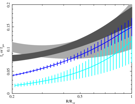
Figure 15.— The radial profile of ${\rm f_{b}}$ and ${\rm f_{gas}}$ for RXJ 1159+5531 (dark grey, dark blue regions, respectively), versus fraction of ${\rm R_{vir}}$. In comparison, we also show the same quantities for the isolated elliptical galaxy NGC 720 (light grey, light blue, respectively). Note the overall similarity in the ${\rm f_{b}}$ profile shape, despite significant discrepancies in ${\rm f_{gas}}$.

We were able to place tight constraints on both the gas and baryon fraction out to the virial radius of the system. While ${\rm f_{gas}}$ rises fairly steeply with radius (so that $\sim$60% of the total gas mass lies outside $\sim$${\rm R_{500}}$), we found that ${\rm f_{b}}$ rises more modestly from $\sim$0.1 at $\sim$100 kpc to approach the Universal baryon fraction (Dunkley et al., 2009; Komatsu et al., 2011) by ${\rm R_{vir}}$. This is consistent with the picture that X-ray bright groups may be baryonically closed (Mathews et al., 2005). Intriguingly, in the isolated, Milky Way-mass elliptical galaxy NGC 720 (almost $\sim$2 orders of magnitude lower in mass), we found a remarkably similar trend. In Fig 15, we compare the profiles for the two systems, scaled with respect to the virial radius. Despite the different ${\rm f_{gas}}$ profiles, ${\rm f_{b}}$ is quite consistent over a wide radial range. Giodini et al. (2009) similarly found a conspiracy between the stellar and gas mass to produce a total baryon fraction at ${\rm R_{500}}$ that is relatively insensitive to the virial mass of the halo. This indicates that, whatever processes are involved in redistributing the baryons in the system, in general the baryons are not being ejected, at least down to $\sim$Milky Way masses.

While ${\rm f_{b}}$ asymptotes to the Universal value by ${\rm R_{vir}}$, the local gas fraction exceeds this limit outside $\sim$${\rm R_{500}}$. Such an enhancement is to be expected if feedback is redistributing baryons in the potential well, but not completely evacuating them from the system. The apparent delicate balance between the gravitational potential and the energy injection from feedback that allows, over a wide range of virial masses, the gas to be pushed out almost to ${\rm R_{vir}}$, but not evacuated from the system, may simply reflect that the mass of gas available to fuel feedback scales with the mass of the system.

Within ${\rm R_{2500}}$ and ${\rm R_{500}}$, our ${\rm f_{gas}}$ measurements were in good agreement with G07, although slightly higher than those found by Vikhlinin et al. (2006) and Sun et al. (2009) (see Fig 9). This reflects a slightly lower gas density found by those authors (e.g. Fig 5), at least within ${\rm R_{2500}}$. These results are also in good accord with similar measurements made in other systems (see Fig 11 of H11), indicating that RXJ 1159+5531, despite being a fossil group, does not experience a highly unusual evolution of its IGrM. In contrast to the outskirts of Perseus, we found no evidence of a systematically over estimated ${\rm f_{gas}}$, which might hint at additional processes such as deviations from hydrostatic equilbrium or sphericity, or clumpiness of the IGrM (Simionescu et al., 2011). The low accretion rate expected for an old fossil group may reduce the impact of these effects in RXJ 1159+5531. We note that we cannot entirely rule out clumping in the outer parts of RXJ 1159+5531, but if present, it must operate in a finely-balanced conspiracy with ${\rm f_{b}}$ in such a manner as to produce a total baryon fraction very close to the cosmological value. In our opinion, such a scenario falls foul of Occam’s razor.

7.4. Entropy profile

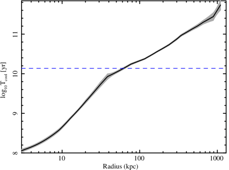
Figure 16.— Cooling time profile of RXJ 1159+5531. Most of the gas in the system has a cooling time longer than the Hubble time (indicated with the dashed line).

The entropy profile of RXJ 1159+5531 shows remarkably similar characteristics to that of other galaxy groups (e.g. Gastaldello et al., 2007a; Mahdavi et al., 2005; Finoguenov et al., 2007; Sun et al., 2009; Cavagnolo et al., 2009; Johnson et al., 2009; Flohic et al., 2011). In the innermost regions, the profile rises steeply (close to $S\propto r^{1.1}$, but offset upwards from the baseline entropy model, Voit et al. 2005), then flattens outside $\sim$0.06${\rm R_{500}}$ (where the cooling time $\sim 10^{10}$Gyr: Fig 16), and converges with the baseline model by $\sim$${\rm R_{500}}$. As expected for hydrostatic gas, S rises monotonically with radius, and we found little evidence of any further breaks in the entropy profile. This overall shape is similar to what is predicted for models in which both stellar winds and AGN contribute to feedback (McCarthy et al., 2010). Significantly, we did not find the characteristic flattening outside $\sim$${\rm R_{500}}$ reported for Perseus and Virgo (Simionescu et al., 2011; Urban et al., 2011), either in the deprojected data, or in our fits with a parameterized model (which had sufficient parameters to capture such behaviour). Therefore, whatever processes are involved in producing such a feature cannot be ubiquitous in massive groups or clusters (or, at least, fossil groups).

As seen in massive galaxy clusters (Pratt et al., 2010), the central parts of groups (Flohic et al., 2011) and the isolated elliptical galaxy NGC 720 (H11), when we scaled the entropy profile by $(f_{gas}/0.17)^{2/3}$, we found it was brought into fairly close agreement with the baseline, adiabatic model (Fig 10). For RXJ 1159+5531, we have now confirmed that this relation holds even out to the virial radius. Taken together with the local ${\rm f_{gas}}$ constraints, it seems that the primary effect of feedback on the baryons is to redistribute the hot gas within the halo, rather than to raise its temperature, or eject it (Mathews & Guo, 2011).

7.5. The pressure profile of RXJ 1159+5531

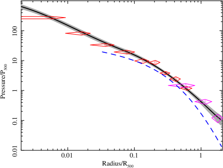
Figure 17.— Pressure profile for RXJ 1159+5531. The dashed blue line is the canonical model of Arnaud et al. (2010).

Recently, it has become evident that the thermal pressure profiles of galaxy clusters and groups, when scaled appropriately, exhibit remarkable uniformity, at least between $\sim$0.5–1.0${\rm R_{500}}$, which has important implications for understanding and calibrating standard scaling relations. Arnaud et al. (2010) proposed a canonical pressure profile model, based on observed clusters within $\sim$${\rm R_{500}}$ and numerical simulations at larger scales. Sun et al. (2011) confirmed that this profile holds for galaxy groups within $\sim$${\rm R_{500}}$. With RXJ 1159+5531, it is now possible to test this model at larger scales. In Fig 17, we show the scaled pressure profile of RXJ 1159+5531, with the canonical model of Arnaud et al. overlaid. At small scales ($\mathrel{\hbox to0.0pt{\lower 3.0pt\hbox{$\sim$}\hss}\raise 2.0pt\hbox{$<$}}$ 0.1${\rm R_{500}}$), there is some disagreement, but this is not unexpected, based on the cluster and group samples. There is general agreement between $\sim$0.2–0.5${\rm R_{500}}$, but the model significantly diverges from the observed pressure distribution at larger scales. Since the global properties of RXJ 1159+5531 are in agreement with standard scaling relations (e.g. Sun et al., 2009), it is unlikely that this represents an artefact of, for example, its fossil group nature. More measurements of the pressure profile out to $\sim$${\rm R_{vir}}$ are clearly needed.

7.6. Constraining the CXB

Despite the data being background dominated at large radius, our results appear to be reasonably robust. This is implied by the well-behaved nature of the density, temperature and mass profiles, the good agreement between the different satellites (in particular, the agreement with the Rosat surface brightness profile), and the reliable measurement of the CXB normalization in our Suzaku fits. Nevertheless, the gas density at the largest scales was sensitive to the precise background, specifically the CXB spectrum (which is the dominant background component). There are, therefore, real concerns that, if the adopted model is not accurate, we may be mis-characterizing the gas properties in the outskirts of the group. As discussed in § 5, one way to mitigate these worries is to employ a Chandra mosaic of the outer Suzaku annuli, enabling us to resolve a large fraction of the CXB component into point sources, from which the CXB shape and normalization can be directly measured. Combining Chandra and Suzaku in this way exploits their complementary capabilities (the high spatial resolution of Chandra; the low instrumental background and good spectral resolution of Suzaku), and should allow the robust detection of gas out to ${\rm R_{vir}}$ to become routine.

8. Conclusions

In our joint Suzaku, Chandra and Rosat analysis of RXJ 1159+5531, we found:

1. By choosing objects with an advantageous combination of distance, mass and surface brightness, it is possible to detect the gas to ${\rm R_{vir}}$ in a single Suzaku pointing. This approach provides better observational efficiency than the multiple pointings needed to mosaic nearby systems, while providing better azimuthal coverage.

2. Applying this approach to the morphologically relaxed fossil group RXJ 1159+5531, we were able to measure the distribution of gas and gravitating matter out to ${\rm R_{vir}}$ for the first time in a system with a mass as low as $10^{14}$${\rm M_{\odot}}$.

3. Within ${\rm R_{vir}}$, the total baryon fraction approached the cosmological value, implying that feedback only redistributed the baryons within the halo, rather than ejecting them.

4. The entropy profile was enhanced over the model from gravity-only cosmological simulations, implying significant feedback. However, outside $\sim$0.06${\rm R_{500}}$, the profile flattened, and converged with the gravity-only model near ${\rm R_{vir}}$. After correcting for the gas fraction, the entropy profile was close to the self-similar predictions of gravitational structure formation simulations, as observed in massive galaxy clusters.

5. In contrast with the Virgo and Perseus clusters, there was no evidence of further flattening in the entropy profile outside $\sim$${\rm R_{500}}$, nor unusually high ${\rm f_{gas}}$ measurements. This indicates that significant gas clumping cannot be ubiquitous near $\sim$${\rm R_{vir}}$, at least for relaxed (fossil) groups.

6. There is good agreement between the best-fitting model for the gas emission and the Chandra, Suzaku and Rosat data, as well as the agreement in the cosmic X-ray background (the dominant background component) measurements made with each satellite.

7. The dominant uncertainty in the gas properties at large radius, the shape CXB spectrum, can be significantly improved upon by using a Chandra mosaic of the outermost Suzaku regions to resolve the CXB into its component point sources so its properties can be constrained directly.

References

- Abadi et al. (2009) Abadi, M. G., Navarro, J. F., Fardal, M., Babul, A., & Steinmetz, M. 2009, arXiv:0902.2477
- Allen et al. (2008) Allen, S. W., Rapetti, D. A., Schmidt, R. W., Ebeling, H., Morris, R. G., & Fabian, A. C. 2008, MNRAS, 383, 879
- Allen et al. (2002) Allen, S. W., Schmidt, R. W., & Fabian, A. C. 2002, MNRAS, 334, L11
- Arnaud (2005) Arnaud, M. 2005, in Background Microwave Radiation and Intracluster Cosmology, ed. F. Melchiorri & Y. Rephaeli, 77
- Arnaud et al. (2010) Arnaud, M., Pratt, G. W., Piffaretti, R., Böhringer, H., Croston, J. H., & Pointecouteau, E. 2010, A&A, 517, A92
- Asplund et al. (2004) Asplund, M., Grevesse, N., & Sauval, J. 2004, in Cosmic abundances as records of stellar evolution and nucleosynthesis, ed. F. N. Bash & T. G. Barnes (ASP Conf. series), astro-ph/0410214
- Bautz et al. (2009) Bautz, M. W., et al. 2009, PASJ, 61, 1117
- Binney & Tremaine (2008) Binney, J. & Tremaine, S. 2008, Galactic Dynamics (2nd ed.; Princeton, NJ: Princeton University Press)
- Blumenthal et al. (1986) Blumenthal, G. R., Faber, S. M., Flores, R., & Primack, J. R. 1986, ApJ, 301, 27
- Böhringer et al. (1994) Böhringer, H., Briel, U. G., Schwarz, R. A., Voges, W., Hartner, G., & Trümper, J. 1994, Nature, 368, 828
- Borgani et al. (2005) Borgani, S., Finoguenov, A., Kay, S. T., Ponman, T. J., Springel, V., Tozzi, P., & Voit, G. M. 2005, MNRAS, 361, 233
- Bryan & Norman (1998) Bryan, G. L. & Norman, M. L. 1998, ApJ, 495, 80
- Bullock et al. (2001) Bullock, J. S., Kolatt, T. S., Sigad, Y., Somerville, R. S., Kravtsov, A. V., Klypin, A. A., Primack, J. R., & Dekel, A. 2001, MNRAS, 321, 559
- Buote (1999) Buote, D. A. 1999, MNRAS, 309, 685
- Buote (2000a) Buote, D. A. 2000a, ApJ, 539, 172
- Buote (2000b) Buote, D. A. 2000b, MNRAS, 311, 176
- Buote et al. (2004) Buote, D. A., Brighenti, F., & Mathews, W. G. 2004, ApJ, 607, L91
- Buote & Fabian (1998) Buote, D. A. & Fabian, A. C. 1998, MNRAS, 296, 977
- Buote et al. (2007) Buote, D. A., Gastaldello, F., Humphrey, P. J., Zappacosta, L., Bullock, J. S., Brighenti, F., & Mathews, W. G. 2007, ApJ, 664, 123
- Buote & Humphrey (2011a) Buote, D. A. & Humphrey, P. J. 2011a, in Hot Interstellar Matter in Elliptical Galaxies, arXiv:1104.0012
- Buote & Humphrey (2011b) Buote, D. A. & Humphrey, P. J. 2011b, MNRAS, submitted (arXiv:1109.6656)
- Buote et al. (2003) Buote, D. A., Lewis, A. D., Brighenti, F., & Mathews, W. G. 2003, ApJ, 594, 741
- Buote & Tsai (1995) Buote, D. A. & Tsai, J. C. 1995, ApJ, 439, 29
- Cash (1976) Cash, W. 1976, A&A, 52, 307
- Cavagnolo et al. (2009) Cavagnolo, K. W., Donahue, M., Voit, G. M., & Sun, M. 2009, ApJS, 182, 12
- Churazov et al. (2008) Churazov, E., Forman, W., Vikhlinin, A., Tremaine, S., Gerhard, O., & Jones, C. 2008, MNRAS, 388, 1062
- De Luca & Molendi (2004) De Luca, A. & Molendi, S. 2004, A&A, 419, 837
- Dickey & Lockman (1990) Dickey, J. M. & Lockman, F. J. 1990, ARA&A, 28, 215
- Dunkley et al. (2009) Dunkley, J., et al. 2009, ApJS, 180, 306
- Eckert et al. (2011) Eckert, D., Molendi, S., Gastaldello, F., & Rossetti, M. 2011, A&A, 529, A133
- Eke et al. (2004) Eke, V. R., et al. 2004, MNRAS, 348, 866
- Fang et al. (2009) Fang, T., Humphrey, P., & Buote, D. 2009, ApJ, 691, 1648
- Feroz & Hobson (2008) Feroz, F. & Hobson, M. P. 2008, MNRAS, 384, 449
- Feroz et al. (2009) Feroz, F., Hobson, M. P., & Bridges, M. 2009, MNRAS, 398, 1601
- Finoguenov & Ponman (1999) Finoguenov, A. & Ponman, T. J. 1999, MNRAS, 305, 325
- Finoguenov et al. (2007) Finoguenov, A., Ponman, T. J., Osmond, J. P. F., & Zimer, M. 2007, MNRAS, 374, 737
- Flohic et al. (2011) Flohic, H. M. L. G. et al. 2011, in preparation
- Gastaldello et al. (2007a) Gastaldello, F., Buote, D. A., Humphrey, P. J., Zappacosta, L., Brighenti, F., & Mathews, W. G. 2007a, in Heating versus Cooling in Galaxies and Clusters of Galaxies, ed. H. Böhringer, G. W. Pratt, A. Finoguenov, & P. Schuecker, 275
- Gastaldello et al. (2007b) Gastaldello, F., Buote, D. A., Humphrey, P. J., Zappacosta, L., Bullock, J. S., Brighenti, F., & Mathews, W. G. 2007b, ApJ, 669, 158
- Gavazzi (2005) Gavazzi, R. 2005, A&A, 443, 793
- George et al. (2009) George, M. R., Fabian, A. C., Sanders, J. S., Young, A. J., & Russell, H. R. 2009, MNRAS, 395, 657
- Giodini et al. (2009) Giodini, S., et al. 2009, ApJ, 703, 982
- Gnedin et al. (2004) Gnedin, O. Y., Kravtsov, A. V., Klypin, A. A., & Nagai, D. 2004, ApJ, 616, 16
- Gnedin et al. (2007) Gnedin, O. Y., Weinberg, D. H., Pizagno, J., Prada, F., & Rix, H.-W. 2007, ApJ, 671, 1115
- Gould (2003) Gould, A. 2003, preprint, astro-ph/0310577
- Graham (2007) Graham, A. W. 2007, MNRAS, 379, 711
- Gultekin et al. (2009) Gultekin, K., et al. 2009, ApJ, 698, 198
- Haiman et al. (2001) Haiman, Z., Mohr, J. J., & Holder, G. P. 2001, ApJ, 553, 545
- Hoshino et al. (2010) Hoshino, A., et al. 2010, PASJ, 62, 371
- Humphrey & Buote (2006) Humphrey, P. J. & Buote, D. A. 2006, ApJ, 639, 136
- Humphrey & Buote (2008) Humphrey, P. J. & Buote, D. A. 2008, ApJ, 689, 983
- Humphrey & Buote (2010) Humphrey, P. J. & Buote, D. A. 2010, MNRAS, 403, 2143
- Humphrey et al. (2008) Humphrey, P. J., Buote, D. A., Brighenti, F., Gebhardt, K., & Mathews, W. G. 2008, ApJ, 683, 161
- Humphrey et al. (2009a) Humphrey, P. J., Buote, D. A., Brighenti, F., Gebhardt, K., & Mathews, W. G. 2009a, ApJ, 703, 1257, (H09)
- Humphrey et al. (2011) Humphrey, P. J., Buote, D. A., Canizares, C. R., Fabian, A. C., & Miller, J. M. 2011, ApJ, 729, 53
- Humphrey et al. (2006) Humphrey, P. J., Buote, D. A., Gastaldello, F., Zappacosta, L., Bullock, J. S., Brighenti, F., & Mathews, W. G. 2006, ApJ, 646, 899, (H06)
- Humphrey et al. (2009b) Humphrey, P. J., Liu, W., & Buote, D. A. 2009b, ApJ, 693, 822
- Ishisaki et al. (2007) Ishisaki, Y., et al. 2007, PASJ, 59, 113
- Jetha et al. (2007) Jetha, N. N., Ponman, T. J., Hardcastle, M. J., & Croston, J. H. 2007, MNRAS, 376, 193
- Johnson et al. (2009) Johnson, R., Ponman, T. J., & Finoguenov, A. 2009, MNRAS, 395, 1287
- Kaastra et al. (2006) Kaastra, J. S., Werner, N., Herder, J. W. A. d., Paerels, F. B. S., de Plaa, J., Rasmussen, A. P., & de Vries, C. P. 2006, ApJ, 652, 189
- Kaiser (1986) Kaiser, N. 1986, MNRAS, 222, 323
- Kawaharada et al. (2010) Kawaharada, M., Okabe, N., Umetsu, K., Takizawa, M., Matsushita, K., Fukazawa, Y., Hamana, T., Miyazaki, S., Nakazawa, K., & Ohashi, T., 2010, ApJ, 714, 423
- Khosroshahi et al. (2007) Khosroshahi, H. G., Ponman, T. J., & Jones, L. R. 2007, MNRAS, 377, 595
- Komatsu et al. (2011) Komatsu, E., et al. 2011, ApJS, 192, 18
- Kraft et al. (2001) Kraft, R. P., Kregenow, J. M., Forman, W. R., Jones, C., & Murray, S. S. 2001, ApJ, 560, 675
- Kriss et al. (1983) Kriss, G. A., Cioffi, D. F., & Canizares, C. R. 1983, ApJ, 272, 439
- Luo et al. (2008) Luo, B., et al. 2008, ApJS, 179, 19
- Macciò et al. (2008) Macciò, A. V., Dutton, A. A., & van den Bosch, F. C. 2008, MNRAS, 391, 1940
- Mahdavi et al. (2005) Mahdavi, A., Finoguenov, A., Böhringer, H., Geller, M. J., & Henry, J. P. 2005, ApJ, 622, 187
- Mathews & Brighenti (2003) Mathews, W. G. & Brighenti, F. 2003, ARA&A, 41, 191
- Mathews et al. (2005) Mathews, W. G., Faltenbacher, A., Brighenti, F., & Buote, D. A. 2005, ApJ, 634, L137
- Mathews & Guo (2011) Mathews, W. G. & Guo, F. 2011, ApJ, 738, 155
- Mazzotta et al. (2004) Mazzotta, P., Rasia, E., Moscardini, L., & Tormen, G. 2004, MNRAS, 354, 10
- McCarthy et al. (2010) McCarthy, I. G., Schaye, J., Ponman, T. J., Bower, R. G., Booth, C. M., Dalla Vecchia, C., Crain, R. A., Springel, V., Theuns, T., & Wiersma, R. P. C. 2010, MNRAS, 406, 822
- McComas et al. (1998) McComas, D. J., Bame, S. J., Barker, P., Feldman, W. C., Phillips, J. L., Riley, P., & Griffee, J. W. 1998, Space Science Reviews, 86, 563
- Nagai & Lau (2011) Nagai, D. & Lau, E. T. 2011, ApJ, 731, L10
- Nagai et al. (2007) Nagai, D., Vikhlinin, A., & Kravtsov, A. V. 2007, ApJ, 655, 98
- Napolitano et al. (2010) Napolitano, N. R., Romanowsky, A. J., & Tortora, C. 2010, MNRAS, in press
- Navarro et al. (1997) Navarro, J. F., Frenk, C. S., & White, S. D. M. 1997, ApJ, 490, 493
- Nomoto et al. (1997a) Nomoto, K., Hashimoto, M., & Tsujimoto, T. 1997a, Nucl. Phys. A, 616, 79
- Nomoto et al. (1997b) Nomoto, K., Iwamoto, K., Nakasoto, N., Thielemann, F. K., Brachwitz, F., Tsujimoto, T., Kubo, Y., & Kishimoto, N. 1997b, Nucl. Phys. A, 621, 467
- Piffaretti et al. (2003) Piffaretti, R., Jetzer, P., & Schindler, S. 2003, A&A, 398, 41
- Piffaretti & Valdarnini (2008) Piffaretti, R. & Valdarnini, R. 2008, A&A, 491, 71
- Ponman et al. (1994) Ponman, T. J., Allan, D. J., Jones, L. R., Merrifield, M., McHardy, I. M., Lehto, H. J., & Luppino, G. A. 1994, Nature, 369, 462
- Ponman et al. (2003) Ponman, T. J., Sanderson, A. J. R., & Finoguenov, A. 2003, MNRAS, 343, 331
- Pratt et al. (2010) Pratt, G. W., Arnaud, M., Piffaretti, R., Böhringer, H., Ponman, T. J., Croston, J. H., Voit, G. M., Borgani, S., & Bower, R. G. 2010, A&A, 511, A85
- Prugniel & Simien (1997) Prugniel, P. & Simien, F. 1997, A&A, 321, 111
- Ptak et al. (2004) Ptak, A., Terashima, Y., Ho, L. C., & Quataert, E. 2004, ApJ, 606, 173
- Purcell et al. (2007) Purcell, C. W., Bullock, J. S., & Zentner, A. R. 2007, ApJ, 666, 20
- Reiprich et al. (2009) Reiprich, T. H., Hudson, D. S., Zhang, Y., Sato, K., Ishisaki, Y., Hoshino, A., Ohashi, T., Ota, N., & Fujita, Y. 2009, A&A, 501, 899
- Simionescu et al. (2011) Simionescu, A., et al. 2011, Science, in press (arXiv:1102.2429)
- Snowden et al. (2004) Snowden, S. L., Collier, M. R., & Kuntz, K. D. 2004, ApJ, 610, 1182
- Springel & Hernquist (2003) Springel, V. & Hernquist, L. 2003, MNRAS, 339, 312
- Sun et al. (2011) Sun, M., Sehgal, N., Voit, G. M., Donahue, M., Jones, C., Forman, W., Vikhlinin, A., & Sarazin, C. 2011, ApJ, 727, L49
- Sun et al. (2009) Sun, M., Voit, G. M., Donahue, M., Jones, C., Forman, W., & Vikhlinin, A. 2009, ApJ, 693, 1142
- Tozzi & Norman (2001) Tozzi, P. & Norman, C. 2001, ApJ, 546, 63
- Tsai et al. (1994) Tsai, J. C., Katz, N., & Bertschinger, E. 1994, ApJ, 423, 553
- Urban et al. (2011) Urban, O., Werner, N., Simionescu, A., Allen, S. W., & Böhringer, H. 2011, MNRAS, in press (arXiv:1102.2430)
- Vikhlinin et al. (2006) Vikhlinin, A., Kravtsov, A., Forman, W., Jones, C., Markevitch, M., Murray, S. S., & Van Speybroeck, L. 2006, ApJ, 640, 691
- Vikhlinin et al. (1999) Vikhlinin, A., McNamara, B. R., Hornstrup, A., Quintana, H., Forman, W., Jones, C., & Way, M. 1999, ApJ, 520, L1
- Voevodkin & Vikhlinin (2004) Voevodkin, A. & Vikhlinin, A. 2004, ApJ, 601, 610
- Voit & Donahue (2005) Voit, G. M. & Donahue, M. 2005, ApJ, 634, 955
- Voit et al. (2005) Voit, G. M., Kay, S. T., & Bryan, G. L. 2005, MNRAS, 364, 909
- Voit & Ponman (2003) Voit, G. M. & Ponman, T. J. 2003, ApJ, 594, L75
- Werner et al. (2008) Werner, N., Durret, F., Ohashi, T., Schindler, S., & Wiersma, R. P. C. 2008, Space Sci. Rev., 134, 337
- White et al. (1993) White, S. D. M., Navarro, J. F., Evrard, A. E., & Frenk, C. S. 1993, Nature, 366, 429
- Young et al. (2011) Young, O. E., Thomas, P. A., Short, C. J., & Pearce, F. 2011, MNRAS, 127
- Zabludoff & Mulchaey (1998) Zabludoff, A. I. & Mulchaey, J. S. 1998, ApJ, 496, 39
- Zezas et al. (2004) Zezas, A., Fabbiano, G., Baldi, A., King, A. R., Ponman, T. J., Raymond, J. C., & Schweizer, F. 2004, in Revista Mexicana de Astronomia y Astrofisica Conference Series, ed. G. Tovmassian & E. Sion, 53–54