A two-Higgs-doublet interpretation of a small Tevatron $Wjj$ excess

Abstract

We show that a $Wjj$ excess in Tevatron data could be explained in the context of the standard non-supersymmetric two-Higgs-doublet model (2HDM) for appropriately chosen parameters. Correlated signals in the $\gamma\gamma$ and $W^{+}W^{-}b\overline{b}$ final states are predicted and are on the verge of being detectable. The proposed model is most attractive if the cross section for the $Wjj$ excess is $\mathrel{\raise 1.29167pt\hbox{$<$\kern-7.5pt\lower 4.30554pt\hbox{$\sim$}}}1-2~{}{\mbox{pb}}$.

The discrepancy between the CDF Aaltonen:2011mk and D0 Abazov:2011rf results implies considerable uncertainty as to whether there is an excess of $Wjj$ events in the $M_{jj}\sim 140~{}{\rm GeV}$ region. Nonetheless, it is interesting to explore the different theoretical approaches that could produce such an excess. Many possibilities have appeared in the literature, including several Higgs sector approaches. A probably incomplete summary is the following: approaches based on $SU(2)$ doublet scalars with or without extra singlets Wang ; Babu ; Dutta:2011kg ; Segre:2011tn ; Chen ; $Z$-prime models Hooper ; Cheung ; new colored state models XPWang ; Dobrescu ; Carpenter:2011yj ; supersymmetry models Kilic ; Sato ; technicolor models Lane ; string theory models stringy ; and within the context of the Standard model He ; Sullivan:2011hu ; Plehn:2011nx . This Letter demonstrates that the excess could be explained by the simplest non-supersymmetric two-Higgs-doublet (2HDM) model with completely standard Yukawa coupling structure. The model predicts correlated signals in the $\gamma\gamma$ and $W^{+}W^{-}b\overline{b}$ final states that are on the verge of detection.

We begin with a general overview of the approach. We employ a two-Higgs-doublet model of Type-II (a convenient summary appears in the HHG hhg ). In the context of the 2HDM, the masses of the light and heavy CP-even Higgs bosons, $h$ and $H$, of the CP-odd Higgs boson, $A$, and of the charged Higgs boson $H^{\pm}$, as well as the value of $\tan\beta=v_{u}/v_{d}$ ($v_{u,d}=\langle H^{0}_{u,d}\rangle$ where $H^{0}_{u,d}$ couple to up-type, down-type quarks, respectively) and the CP-even Higgs sector mixing angle $\alpha$ can all be taken as independent parameters, whose values will determine the $\lambda_{i}$ of the general 2HDM Higgs potential.

To obtain a $Wjj$ signal with Tevatron cross section of order $\mathrel{\raise 1.29167pt\hbox{$>$\kern-7.5pt\lower 4.30554pt\hbox{$\sim$}}}1~{}{\mbox{pb}}$, the first ingredient is to note that the cross section for $gg\rightarrow A$ is highly enhanced at a given $m_{A}$ relative to the cross section for a SM Higgs boson at $m_{h_{SM}}=m_{A}$ when $\tan\beta<1$. The $Wjj$ signal derives from the (dominant) $A\rightarrow H^{\pm}W^{\mp}$ decay channel with $H^{\pm}\rightarrow cs$. Note that this particular mode does not contain $b$ quarks, as consistent with the CDF observations. Using the predicted value of $BR(H^{+}\rightarrow cs)\sim 0.2$ for $m_{H^{\pm}}\sim 140~{}{\rm GeV}$ when $\tan\beta$ is small, one finds that a cross section for $gg\rightarrow A\rightarrow H^{\pm}W^{\mp}\rightarrow csW^{\mp}$ as large as the CDF value of $\sim 4~{}{\mbox{pb}}$ can only be achieved for $m_{A}\in[250,300]~{}{\rm GeV}$ if $\tan\beta\mathrel{\raise 1.29167pt\hbox{$<$\kern-7.5pt\lower 4.30554pt\hbox{$\sim$}}}1/10$, a domain for which the top-quark Yukawa coupling is non-perturbative, $\alpha_{t}\equiv\lambda_{t}^{2}/(4\pi)>1$. However, a smaller $Wjj$ cross section of order $1-2~{}{\mbox{pb}}$ is possible for $\alpha_{t}\sim 1$. We now present more details.

In the 2HDM there are only two possible models for the fermion couplings that naturally avoid flavor changing neutral currents (FCNC), Model I and Model II. In Model II, our focus here, the tree-level couplings of the Higgs bosons are:

$$\begin{array}[]{|c|c|c|c|}\hline\cr&h&H&A\cr\hline\cr t\overline{t}&{\cos\alpha\over\sin\beta}&{\sin\alpha\over\sin\beta}&-i\gamma_{5}\cot\beta\cr\hline\cr b\overline{b}&-{\sin\alpha\over\cos\beta}&{\cos\alpha\over\cos\beta}&-i\gamma_{5}\tan\beta\cr\hline\cr WW,ZZ&\sin(\beta-\alpha)&\cos(\beta-\alpha)&0\cr\hline\cr\end{array}\vspace*{-.12in}$$ (1)

We will fix $\alpha$ relative to $\beta$ by requiring that the $h$ be SM-like, i.e. $\sin(\beta-\alpha)=1$. We also choose $m_{h}=115~{}{\rm GeV}$ for easy consistency with precision electroweak data. If the $\lambda_{i}$ of the Higgs potential are kept highly perturbative, the decoupling limit, in which $m_{H},m_{H^{\pm}}\rightarrow m_{A}$ and $\sin^{2}(\beta-\alpha)\rightarrow 1$, sets in fairly quickly as $m_{A}$ increases Gunion:2002zf . To describe a $Wjj$ excess requires that $m_{H^{\pm}}<m_{A}$ (but $m_{H}\sim m_{A}$ is useful to enhance the signal), implying that the decoupling limit does not apply at the masses of interest. This requires that several of the $\lambda_{i}$ are substantial but still below the $\lambda_{i}^{2}/(4\pi)\sim 1$ beginning of the non-perturbative domain.

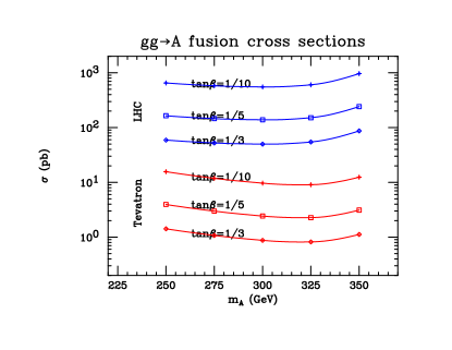
Figure 1: Tevatron and LHC cross sections for $gg\rightarrow A$ for representative $\tan\beta<1$ values.

Looking at Eq. (1), it is apparent that the cross section for $gg\rightarrow A$ can be large when $\cot\beta>1$. It is also useful to recall that the fermionic loop function for the $A$ is substantially larger than that for the $H$ (the CP-even Higgs that could contribute to the $Wjj$ excess if the $h$ is SM-like); e.g. asymptotically $F_{1/2}^{A}(\tau)\rightarrow 2$ in comparison to $F_{1/2}^{H}(\tau)\rightarrow-4/3$ when $\tau=4m_{f}^{2}/m_{A}^{2}\rightarrow\infty$, implying a cross section gain by a factor of $9/4$ for $A$ vs. the $H$ in the heavy fermion mass limit. We have computed the $gg\rightarrow A$ (and $gg\rightarrow H$) cross section using HIGLU Spira:1996if and a private program and obtained essentially the same results. Results for $\sigma(gg\rightarrow A)$ are plotted in Fig. 1. These results include NLO and NNLO corrections as in HIGLU. Some useful benchmark numbers for $m_{A}=250~{}{\rm GeV}$ are

$$\begin{array}[]{|l|l|l|l|}\hline\cr\tan\beta&1/3&1/5&1/10\cr\hline\cr\sigma(gg\rightarrow A)_{Tevatron}&1.4~{}{\mbox{pb}}&3.9~{}{\mbox{pb}}&15.7~{}{\mbox{pb}}\cr\hline\cr\sigma(gg\rightarrow A)_{LHC}&59.1~{}{\mbox{pb}}&164.3~{}{\mbox{pb}}&652.9~{}{\mbox{pb}}\cr\hline\cr\end{array}$$ (2)

Figure 2: $BR(H^{+}\rightarrow c\overline{s})$ (solid blue) and $BR(H^{+}\rightarrow t\overline{b})$ (red dots) as a function of $\tan\beta$ for $m_{H^{\pm}}=140~{}{\rm GeV}$ and Model II couplings. Inclusion of off-shell decay configurations is essential for the $t\overline{b}$ final state.

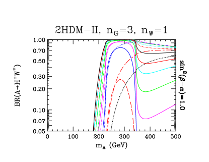
Figure 3: $BR(A\rightarrow H^{\pm}W^{\mp})$ as a function of $m_{A}$ for $m_{H^{\pm}}=140~{}{\rm GeV}$ and Model II couplings. In this and subsequent plot for the $A$, we have taken $m_{H}=140~{}{\rm GeV}$. The legend is as follows: solid black$\rightarrow\tan\beta=1$; red dots$\rightarrow\tan\beta=1.5$; solid red$\rightarrow\tan\beta=1/1.5$; cyan dots$\rightarrow\tan\beta=2$; solid cyan$\rightarrow\tan\beta=1/2$; green dots$\rightarrow\tan\beta=3$; solid green$\rightarrow\tan\beta=1/3$; magenta dots$\rightarrow\tan\beta=5$; solid magenta$\rightarrow\tan\beta=1/5$; blue dots$\rightarrow\tan\beta=10$; solid blue$\rightarrow\tan\beta=1/10$; long red dashes plus dots$\rightarrow\tan\beta=30$; pure long red dashes$\rightarrow\tan\beta=1/30$; black dotdash$\rightarrow\tan\beta=50$. This and subsequent figures must be viewed in color in order to resolve the different $\tan\beta$ cases. Results plotted include off-shell decay configurations. $n_{G}=3$, $n_{W}=1$ means 3 generations, no sequential $W^{\prime}$.

We define the effective $Wjj$ cross section for a Higgs boson $X$:

$$\sigma_{Wjj}^{X}\equiv BR(X\rightarrow H^{\pm}W^{\mp})BR(H^{+}\rightarrow c\overline{s})\sigma(gg\rightarrow X),$$ (3)

where $X=A$ and $X=H$ are the relevant Higgs bosons. As a benchmark to keep in mind, we will suppose that $\sigma_{Wjj}^{A}\sim 1~{}{\mbox{pb}}$ is appropriate for describing the Tevatron $Wjj$ excess. $BR(H^{+}\rightarrow c\overline{s})$ (computed privately and using HDECAY Djouadi:1997yw ) is displayed in Fig. 2 where we see that a value of $\sim 0.22$ applies for $\tan\beta\in[1/10,1/3]$. For $m_{A}=250~{}{\rm GeV}$, Fig. 3 shows that $BR(A\rightarrow H^{\pm}W^{\mp})\sim 0.95,0.874,0.64$ for $\tan\beta=1/3,1/5,1/10$ (the solid green, magenta, blue lines), respectively. For $m_{A}=250~{}{\rm GeV}$ we then obtain $BR(A\rightarrow H^{\pm}W^{\mp})BR(H^{+}\rightarrow c\overline{s})\sim 0.21,0.19,0.14$ for $\tan\beta=1/3,1/5,1/10$. Using the $\sigma(gg\rightarrow A)$ cross sections of Eq. (2), for $m_{A}=250~{}{\rm GeV}$ we find $\sigma_{Wjj}^{A}(Tevatron)\sim 0.3~{}{\mbox{pb}},\ 0.75~{}{\mbox{pb}},\ 2.2~{}{\mbox{pb}}$ for $\tan\beta=1/3,\ 1/5,\ 1/10$, respectively. The corresponding values of $\alpha_{t}$ are $0.63,\ 1.75,\ 7$. Only the latter is uncomfortably (but not drastically) non-perturbative, implying a preference for $\sigma_{Wjj}^{A}\mathrel{\raise 1.29167pt\hbox{$<$\kern-7.5pt\lower 4.30554pt\hbox{$\sim$}}}1~{}{\mbox{pb}}$. It is quite important to note that the main reason that $\sigma_{Wjj}^{A}$ is not larger is the small value of $BR(H^{+}\rightarrow c\overline{s})$ that is a consequence of the dominance of off-shell $H^{+}\rightarrow t^{*}\overline{b}$ decays for $m_{H^{\pm}}=140~{}{\rm GeV}$. (This dominance decreases rapidly if $m_{H^{\pm}}$ is decreased; for $m_{H^{\pm}}$ significantly lower that $140~{}{\rm GeV}$ higher $\sigma_{Wjj}^{A}$ would thus be achieved.) For $m_{A}\mathrel{\raise 1.29167pt\hbox{$>$\kern-7.5pt\lower 4.30554pt\hbox{$\sim$}}}300~{}{\rm GeV}$, $\sigma_{Wjj}^{A}$ is about 50% smaller than the $m_{A}=250~{}{\rm GeV}$ values quoted above, see Fig. 1.

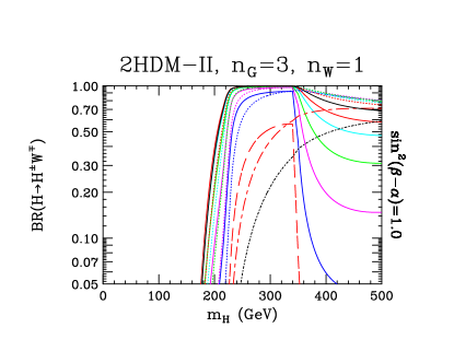
Figure 4: $BR(H\rightarrow H^{\pm}W^{\mp})$ as a function of $m_{A}$ for $m_{H^{\pm}}=140~{}{\rm GeV}$ and Model II couplings. In this and subsequent plots for the $H$, we have taken $m_{A}=200~{}{\rm GeV}$. The legend is as in Fig. 3.

As apparent from Eq. (2), $\sigma(gg\rightarrow A)$ is much larger at the LHC. Focusing on $m_{A}=250~{}{\rm GeV}$ and including the earlier quoted $BR(A\rightarrow H^{\pm}W^{\mp})BR(H^{+}\rightarrow c\overline{s})$ values of $0.21,\ 0.19,\ 0.14$ we obtain $\sigma_{Wjj}^{A}(LHC)=12.4~{}{\mbox{pb}},\ 31.2~{}{\mbox{pb}},\ 91.4~{}{\mbox{pb}}$ for $\tan\beta=1/3,\ 1/5,\ 1/10$, respectively. The number of $Wjj$ events will be enormous for the soon-to-be-achieved $L=1~{}{\mbox{fb}^{-1}}$. We anxiously await the appropriate LHC analyzes.

It is, of course, interesting to assess the extent to which $gg\rightarrow H\rightarrow H^{\pm}W^{\mp}$ with $H^{+}\rightarrow c\overline{s}$, $H^{-}\rightarrow\overline{c}s$ could contribute to the $Wjj$ final state (recall that the $h$ is taken to be light and SM-like so that only the $H$ is relevant for the $Wjj$ excess). We have already noted that $\sigma_{Wjj}^{H}<\sigma_{Wjj}^{A}$ due to the smaller fermionic loop function. Actual ratios at the Tevatron are: $\sigma_{Wjj}^{A}/\sigma_{Wjj}^{H}\sim 2.6,\ 3.0,\ 5.0$ for $m_{A}=m_{H}=250,\ 300,\ 350~{}{\rm GeV}$. Meanwhile, the $BR(H\rightarrow H^{\pm}W^{\mp})BR(H^{+}\rightarrow c\overline{s})$ values are similar to those quoted for the $A$. Thus, for the preferred $m_{H}\in[250-300]~{}{\rm GeV}$ mass range, the $H$ would yield a $Wjj$ signal of order $30\%-40\%$ of the $A$ result. If the $H$ and $A$ are not fairly degenerate, this would yield a somewhat spread out net $Wjj$ signal, despite the $\mathrel{\raise 1.29167pt\hbox{$<$\kern-7.5pt\lower 4.30554pt\hbox{$\sim$}}}1~{}{\rm GeV}$ total widths of the $A$ and $H$ (for the $\tan\beta$ values being discussed), given the experimental $M_{jj}$ resolution of order $15~{}{\rm GeV}$. This is perhaps suggested by the absence of any distinct peaking in the $Wjj$ mass in the data. Another interesting point is that in this model with $m_{H}$ not very different from $m_{A}$, there would be no signal in the $Zjj$ channel due to the absence of $H\rightarrow AZ$ and $A\rightarrow HZ$ decays.

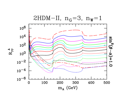
Figure 5: $R_{\gamma\gamma}$ for the 2HDM-II $A$. The legend is as in Fig. 3. This figure takes account of all the $A$ decay modes, including especially $A\rightarrow H^{\pm}W^{\mp}$ as well as $A\rightarrow t\overline{t}$ (off-shell) decays.

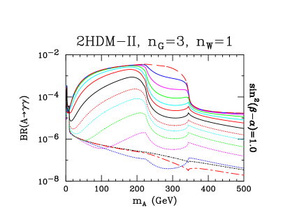
Figure 6: $BR(A\rightarrow\gamma\gamma)$ for the 2HDM-II $A$ after including $A\rightarrow H^{\pm}W^{\mp}$ and $A\rightarrow t\overline{t}$ off-shell decays in the present scenario. The legend is as in Fig. 3.

Other signals should be seen if the model is correct. In particular, as pointed out in Gunion:2011ww , there is a very large $A\rightarrow\gamma\gamma$ signal for small $\tan\beta$. A plot of $R_{\gamma\gamma}^{A}\equiv[\Gamma_{gg}^{A}BR(A\rightarrow\gamma\gamma)]/[\Gamma_{gg}^{h_{SM}}BR(h_{SM}\rightarrow\gamma\gamma)]$ is given in Fig. 5. For $\tan\beta\sim 1/3,1/5$ and $m_{A}\sim 250~{}{\rm GeV}$, $R_{\gamma\gamma}^{A}\sim 10^{2},10^{3}$, respectively! Such a signal will soon be observed at the LHC if present and might also be observable with current Tevatron data. To assess actual event rates one can combine the actual branching ratio for $A\rightarrow\gamma\gamma$, plotted in Fig. 6 with the cross sections for $gg\rightarrow A$ plotted in Fig. 1.

For example, for $\tan\beta=1/5$ and $m_{A}=250~{}{\rm GeV}$, in the case of the Tevatron one finds $\sigma(gg\rightarrow A)BR(A\rightarrow\gamma\gamma)\sim 3.9~{}{\mbox{pb}}\times 4.8\cdot 10^{-4}\simeq 1.9\times 10^{-3}~{}{\mbox{pb}}$, yielding $\sim 10$ events for $L=5.4~{}{\mbox{fb}^{-1}}$. This must be compared to the number of events expected in the SM. Ref. Aaltonen:2010cf performs an analysis for $L=5.4~{}{\mbox{fb}^{-1}}$. Their net efficiency times acceptance is $\sim 0.12$, implying a predicted number of $A\rightarrow\gamma\gamma$ events of order $1.2$. The actual number of observed events is consistent with the SM prediction, as shown in their Fig. 2. They set a 95% CL limit of $\sigma BR(\gamma\gamma)\mathrel{\raise 1.29167pt\hbox{$<$\kern-7.5pt\lower 4.30554pt\hbox{$\sim$}}}0.05~{}{\mbox{pb}}$ at $M_{\gamma\gamma}=250~{}{\rm GeV}$, a factor of $\sim 25$ above our typical prediction. At the LHC, the corresponding calculation is $\sigma(gg\rightarrow A)BR(A\rightarrow\gamma\gamma)\sim 164~{}{\mbox{pb}}\times 4.8\cdot 10^{-4}=0.08~{}{\mbox{pb}}$. For $L=36~{}\mbox{pb}^{-1},1~{}{\mbox{fb}^{-1}}$ this yields $\sim 3,80$ events, respectively. Ref. cmsgravitonstudy uses $L=36~{}\mbox{pb}^{-1}$ data to set a limit of $\sigma\times BR(\gamma\gamma)\mathrel{\raise 1.29167pt\hbox{$<$\kern-7.5pt\lower 4.30554pt\hbox{$\sim$}}}0.7~{}{\mbox{pb}}$ at $M_{\gamma\gamma}=250~{}{\rm GeV}$, a factor of about $8$ above the prediction for the present scenario. This shows that the present scenario for obtaining a $Wjj$ excess will be strongly tested once the currently available LHC data sets with $L=1~{}{\mbox{fb}^{-1}}$ are analyzed.

Of course, the $H$ also yields a large $\gamma\gamma$ signal (again of order $30\%-40\%$ that of the $A$) that most probably would be detected as a separate peak if $m_{H}$ differs from $m_{A}$ by more than $10~{}{\rm GeV}$, given the excellent $\sim 2~{}{\rm GeV}$ mass resolution in $M_{\gamma\gamma}$ for the LHC detectors and given that the total $A$ and $H$ widths are of order $1~{}{\rm GeV}$.

Finally, there is an interesting signal in the $gg\rightarrow A\rightarrow H^{\pm}W^{\mp}\rightarrow t^{*}\overline{b}W^{-}+\overline{t}^{*}bW^{+}$ final state deriving from the $BR(H^{+}\rightarrow t^{*}\overline{b})\sim 0.7$ (off-shell) decays, see Fig. 2, where $t^{*}\rightarrow W^{+}b$. The resulting final states of $W^{+}W^{-}b\overline{b}$ will not peak in either $Wb$ mass combination. The cross section for this final state is, however, significant: for $m_{A}=250~{}{\rm GeV}$ and $\tan\beta=1/5$, one finds $\sigma(WWbb)\sim 2.8~{}{\mbox{pb}}$ compared to $\sigma_{Wjj}^{A}\sim 0.75~{}{\mbox{pb}}$ and $\sigma_{Wjj}^{H}\sim 0.28~{}{\mbox{pb}}$. Although this $\sigma(WWbb)$ is somewhat smaller than that for direct $t\overline{t}\rightarrow W^{+}W^{-}b\overline{b}$ production, it is still sizable and might lead to some “anomalies” in the $W^{+}W^{-}b\overline{b}$ final state. It would be very interesting to determine whether or not such anomalies in the $W^{+}W^{-}b\overline{b}$ final state would have been noticed in current data and, if not, how much LHC integrated luminosity would be needed to detect them. One should note that for this model to achieve the CDF $Wjj$ cross section of $\sim 4~{}{\mbox{pb}}$ would imply an anomalous $W^{+}W^{-}b\overline{b}$ final state cross section that is larger than that coming directly from $t\overline{t}\rightarrow W^{+}W^{-}b\overline{b}$ production.

If a 4th generation is present with $m_{t^{\prime},b^{\prime}}\sim 400~{}{\rm GeV}$, then $\Gamma_{gg}^{A}$ and, therefore, $\sigma_{Wjj}^{A}$ is increased substantially at any fixed $\tan\beta$. However, $\tan\beta$ is restricted to lie in the range $\tan\beta\in[1/2,2]$ in order to keep $\lambda_{t^{\prime},b^{\prime}}^{2}/(4\pi)\mathrel{\raise 1.29167pt\hbox{$<$\kern-7.5pt\lower 4.30554pt\hbox{$\sim$}}}1$. The resulting $gg\rightarrow A$ rate is then more or less the same as for $\tan\beta\in[1/3,1/5]$ with no 4th generation.

Enhanced $gg\rightarrow A$ cross sections also arise in a Model I 2HDM if $\tan\beta<1$. However, the enhancement is not quite as great as for Model II. In addition, $BR(H^{+}\rightarrow c\overline{s})\sim 0.13$ for $\tan\beta\in[1/3,1/10]$. As a result, the $Wjj$ cross section that can be achieved in Model I is smaller by about a factor of three as compared to that achieved for the $Wjj$ final state in the case of Model II.

To summarize, we have shown that if $\tan\beta$ is small then a Model II two-Higgs-doublet sector with $m_{A}$, and possibly $m_{H}$, of order $250~{}{\rm GeV}-300~{}{\rm GeV}$ can lead to a very interesting signal in the $Wjj$ final state that could match that seen by CDF at the Tevatron. To get a cross section as large as that originally claimed by CDF would force one to $\tan\beta\mathrel{\raise 1.29167pt\hbox{$<$\kern-7.5pt\lower 4.30554pt\hbox{$\sim$}}}1/10$, values for which the top-quark Yukawa coupling is quite large and moderately non-perturbative. However, a $Wjj$ signal with cross section of order $1~{}{\mbox{pb}}$, as possibly consistent with a combination of CDF and D0 data, is quite possible without entering into the domain of non-perturbative top-quark Yukawas. Correlated signals in the $W^{+}W^{-}b\overline{b}$ and $\gamma\gamma$ final states are expected. These final states are interesting targets for exploration in their own right. The predicted correlations between the $Wjj$, $W^{+}W^{-}b\overline{b}$ and $\gamma\gamma$ signals makes the model proposed herein highly testable and points out the importance of taking into account the latter types of signals in order to fully assess the consistency of the model. At the LHC, the predicted $Wjj$ cross sections and those for the correlated signals are of order 40 times as large as at the Tevatron. As the integrated LHC luminosity approaches $L=1~{}{\mbox{fb}^{-1}}$ the model will most probably be definitively eliminated or confirmed. As a final note, the masses for the $m_{H^{\pm}}$, $m_{A}$ and $m_{H}$ needed to explain the possible $Wjj$ excess using the approach described here cannot be achieved within the minimal supersymmetric model context.

References

(1)
T. Aaltonen et al. [ CDF Collaboration ],
Phys. Rev. Lett. 106, 171801 (2011),
arXiv:1104.0699.
(2)
V. M. Abazov et al. [ D0 Collaboration ],
arXiv:1106.1457.
(3)
Q. H. Cao, M. Carena, S. Gori, A. Menon, P. Schwaller, C. E. M. Wagner and L. T. M. Wang,
arXiv:1104.4776.
(4)
K. S. Babu, M. Frank, S. K. Rai,
arXiv:1104.4782.
(5)
B. Dutta, S. Khalil, Y. Mimura, Q. Shafi,
arXiv:1104.5209.
(6)
G. Segre, B. Kayser,
arXiv:1105.1808.
(7)
C. H. Chen, C. W. Chiang, T. Nomura and Y. Fusheng,
arXiv:1105.2870.
(8)
M. R. Buckley, D. Hooper, J. Kopp and E. Neil,
arXiv:1103.6035.
(9)
K. Cheung and J. Song,
arXiv:1104.1375.
(10)
X. P. Wang, Y. K. Wang, B. Xiao, J. Xu and S. h. Zhu,
arXiv:1104.1917.
(11)
B. A. Dobrescu and G. Z. Krnjaic,
arXiv:1104.2893.
(12)
L. M. Carpenter, S. Mantry,
arXiv:1104.5528.
(13)
C. Kilic and S. Thomas,
arXiv:1104.1002.
(14)
R. Sato, S. Shirai and K. Yonekura,
arXiv:1104.2014.
(15)
E. J. Eichten, K. Lane and A. Martin,
arXiv:1104.0976.
(16)
L. A. Anchordoqui, H. Goldberg, X. Huang, D. Lust and T. R. Taylor,
arXiv:1104.2302.
(17)
X. G. He and B. Q. Ma,
arXiv:1104.1894.
(18)
Z. Sullivan, A. Menon,
arXiv:1104.3790.
(19)
T. Plehn, M. Takeuchi,
arXiv:1104.4087.
(20)The Higgs Hunters Guide,
John F. Gunion, Howard E. Haber, Gordon Kane, Sally Dawson. 1990.
Series: Frontiers in Physics, 80; QCD161:G78
(21)
J. F. Gunion, H. E. Haber,
Phys. Rev. D67, 075019 (2003),
[hep-ph/0207010].
(22)
M. Spira,
Nucl. Instrum. Meth. A 389, 357 (1997)
[arXiv:hep-ph/9610350],
arXiv:hep-ph/9510347.
(23)
A. Djouadi, J. Kalinowski, M. Spira,
Comput. Phys. Commun. 108, 56-74 (1998),
[hep-ph/9704448].
(24)
J. F. Gunion,
arXiv:1105.3965.
(25)
T. Aaltonen et al. [ CDF Collaboration ],
Phys. Rev. D83, 011102 (2011).
[arXiv:1012.2795].