PACS Evolutionary Probe (PEP) - A Herschel Key Program

Deep far-infrared photometric surveys studying galaxy evolution and the nature of the cosmic infrared background are a key strength of the Herschel mission. We describe the scientific motivation for the PACS Evolutionary Probe (PEP) guaranteed time key program and its role in the complement of Herschel surveys, and the field selection which includes popular multiwavelength fields such as GOODS, COSMOS, Lockman Hole, ECDFS, EGS. We provide an account of the observing strategies and data reduction methods used. An overview of first science results illustrates the potential of PEP in providing calorimetric star formation rates for high redshift galaxy populations, thus testing and superseeding previous extrapolations from other wavelengths, and enabling a wide range of galaxy evolution studies.

1 Motivation

Over the last two decades, it has become increasingly clear that no understanding of galaxy evolution can be obtained without accounting for the energy that is absorbed by dust and re-emitted at mid- and far-infrared wavelengths. For example, early attempts to reconstruct the cosmic star formation history suffered from uncertainties in the obscuration corrections that have to be applied to the rest frame ultraviolet measurements (e.g. Madau madau96 (1996), Lilly et al. lilly96 (1996)). Soon, the importance of luminous dusty high redshift galaxies was highlighted by the detection of infrared-luminous populations both in the mid-infrared (e.g. Aussel et al. aussel99 (1999), Genzel & Cesarsky genzel00 (2000)) and the submm (e.g. Hughes et al. hughes98 (1998)). Mainly due to the large mid-infrared legacy that the Spitzer mission provided for extragalactic studies (Soifer et al. soifer08 (2008)), a global consistency between these two perspectives from the rest frame ultraviolet and from the rest frame mid-IR side could be achieved (e.g. Hopkins and Beacom hopkins06 (2006)). This is because the rest frame ultraviolet obscuration on average can be constrained by comparing the observed ultraviolet emission to the sum of ultraviolet and infrared emission. Extrapolation from the mid-infrared to the rest far-infrared was still necessary, however, on the basis of SED assumptions that were untested at the redshifts to which they had to be applied.

At the same time, the detection of the cosmic far-infrared background (CIB) with total energy content similar to the optical/near-infrared one (Puget et al. puget96 (1996), Hauser et al. hauser98 (1998)) highlighted the importance of dust emission in the cosmic energy budget. An increase with redshift in the energy output of dusty galaxies relative to others was inferred both from the shape of the CIB and from the more rapid increase with redshift of IR energy density compared to ultraviolet energy density in the resolved observations (e.g., Le Floc’h lefloch05 (2005)). All these lines of evidence strongly suggest that our picture of high redshift galaxy evolution is substantially incomplete and emphasize the need for direct rest frame ‘calorimetric’ far-infrared measurements of individual high-z galaxies, in order to avoid SED extrapolation and to increasingly replace population averages with individual measurements. While small cryogenic space telescopes like ISO and Spitzer were already equipped with sensitive far-infrared detectors, they were for these wavelengths rapidly limited by source confusion, and thus focussed on the study of local objects, or at z$\gtrsim$0.5 on study of only the most luminous galaxies. They also were able to resolve only a small fraction of the cosmic infrared background.

Table 1: PEP fields

Field	RA	DEC	Size	PA	wavelengths	Observations	Time
	degree, J2000		arcmin	degree	$\mu$m		hours
COSMOS	150.11917	2.20583	85$\times$85	0	100,160	Nov 2009 – Jun 2010	196.9
Lockman Hole XMM	163.17917	57.48000	24$\times$24	0	100,160	Oct 2009 – Nov 2009	32.1
EGS	214.82229	52.82617	67$\times$10	40.5	100,160	May 2011 – June 2011	34.8
ECDFS	53.10417	-27.81389	30$\times$30	0	100,160	Feb 2010 – Feb 2011	32.8
GOODS-S	53.12654	-27.80467	17$\times$11	-11.3	70,100,160	Jan 2010	239.7
GOODS-N	189.22862	62.23867	17$\times$11	41	100,160	Oct 2009	25.8
Cl0024+16	6.62500	17.16250	6$\times$6	45	100,160	Jun 2010	6.2
Abell 370	39.97083	-1.57861	4$\times$4	45	100,160		5.3
MS0451.6-0305	73.55000	-3.01667	4$\times$4	45	100,160	May 2010	5.3
Abell 1689	197.87625	-1.34000	4$\times$4	45	100,160	Jan 2011 –	13.0
RXJ1347.5-1145	206.87708	-11.75250	4$\times$4	45	100,160	Feb 2011	5.3
MS1358.4+6245	209.97625	62.51000	4$\times$4	45	100,160	May 2010	5.3
Abell 1835	210.25833	2.87889	4$\times$4	45	100,160	Feb 2011	5.3
Abell 2218	248.97083	66.20611	4$\times$4	45	100,160	Oct 2009	10.2
Abell 2219	250.08333	46.71194	4$\times$4	45	100,160	May 2010	5.3
Abell 2390	328.40417	17.69556	4$\times$4	45	100,160	May 2010	5.3
RXJ0152.7-1357	38.17083	-13.96250	10$\times$5	45	100,160,250,350,500	Mar 2010 – Jan 2011	5.8
MS1054.4-0321	164.25092	-3.62428	10$\times$5	0	100,160,250,350,500	Jun 2010 – Dec 2010	5.8

With ESA’s Herschel space observatory (Pilbratt pilbratt10 (2010)) and its PACS (Poglitsch et al. poglitsch10 (2010)) and SPIRE (Griffin et al. griffin10 (2010)) instruments, this has changed dramatically. With its 3.5 m passively cooled mirror it provides the much improved spatial resolution (thus reduced source confusion) and the sensitivity needed for the next significant step in far-infrared studies of galaxy evolution. Members of the PACS instrument consortium, the Herschel Science Centre and mission scientist M. Harwit have joined forces in the PACS Evolutionary Probe (PEP) deep extragalactic survey, to make use of this opportunity. PEP aims to resolve the cosmic infrared background and determine the nature of its constituents, determine the cosmic evolution of dusty star formation and of the infrared luminosity function, elucidate the relation of far-infrared emission and environment and determine clustering properties. Other main goals include study of AGN/host coevolution, and determination of the infrared emission and energetics of known high redshift galaxy populations.

PEP encompasses deep observations of blank fields and lensing clusters, close to the Herschel confusion limit, in order to probe down to representative high redshift galaxies, rather than being restricted to individually interesting extremely luminous cases. PEP is focussed on PACS 70, 100, and 160 $\mu$m observations. SPIRE observations of the PEP fields are obtained in coordination with PEP by the HerMES survey (Oliver et al. oliver11 (2011)). Larger and shallower fields are observed by HerMES (70 deg²) as well as by the H-ATLAS survey (570 deg², Eales et al. eales10 (2010)), while the GOODS-Herschel program (Elbaz et al. elbaz11 (2011)) provides deeper observation in (part of) the GOODS fields that are also covered by PEP. Finally, the Herschel lensing survey (Egami et al. egami10 (2010)) substantially increases the number of lensing clusters observed with Herschel, adding about 40 clusters to the 10 objects covered by PEP. Fig. 1 compares for 160$\mu$m wavelength the area and exposure of the PEP surveys (Table 1) with that of these other major Herschel extragalactic surveys.

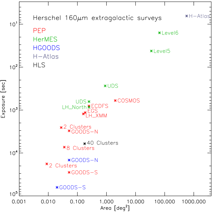
Figure 1: Area and 160$\mu$m exposure of PEP surveys (red) compared to other major Herschel extragalactic surveys. Exposure is defined as survey time (including overheads) multiplied with the ratio of PACS array size and survey area. 1000 sec exposure corresponds to an approximate 3$\sigma$ depth of 8 mJy. Scaling this as exposure^-0.5 to smaller/deeper fields will be too optimistic because of increasing overhead fractions and beginning source confusion.

In this paper, we describe the field selection, observing strategy and data analysis methods of PEP. We give a complete overview of the planned PEP observations and their execution status as of June 2011 (Table 1). We provide a detailed account of the science demonstration phase (SDP) data sets for GOODS-N and Abell 2218, and give an overview of first science results.

2 Field selection

A key element in selecting a field for a deep Herschel extragalactic survey is the availability of a strong multi-wavelength database from X-rays to radio wavelengths, which is fundamental to many of the science results discussed in Sect. 6. In particular, deep optical, near-IR, and Spitzer imaging, as well as a comprehensive set of photometric and spectroscopic redshifts are an essential asset for most of the far-infrared studies of galaxy evolution that we envisage. Deep X-ray data are invaluable for using the potential of Herschel for studying the AGN – host galaxy coevolution.

Another requirement is a low galactic far-infrared background in order to minimize contamination by galactic ‘cirrus’ structure and by individual galactic foreground objects. This naturally coincides with the selection criteria of extragalactic surveys at other wavelengths. In the X-ray regime, for example, these are pushing for a low galactic foreground obscuration. Given that the power spectra of far-infrared emission of galactic cirrus are steeply decreasing towards higher spatial frequencies (e.g., Kiss et al. kiss01 (2001)), such cirrus contamination is much less of a practical worry for point source detection in deep Herschel fields compared to the previous smaller cryogenic space telescopes. In any case, our blank field selection includes some of the lowest galactic foreground fields (Lockman Hole, CDFS, 100 $\mu$m sky brightness $\sim$0.4 MJy/sr), reaching up to $\sim$0.9 MJy/sr (COSMOS). Our individual cluster fields typically show a 100 $\mu$m galactic foreground of 1-2 MJy/sr, with a maximum of 4.5 MJy/sr (Abell 2390).

Table 2: AOR parameters used for the PEP fields

Field	Nominal scan direction							Orthogonal scan direction
	Leg	Step	NL	Angle		NRep	NAOR	Leg	Step	NL	Angle		NRep	NAOR
	′	″		°				′	″		°
COSMOS	85	Hom	Sq	70	Arr	1	24	85	Hom	Sq	160	Arr	2	25
Lockman Hole XMM	24	50	30	0	Sky	2	10	24	50	30	90	Sky	2	10
EGS	67	50	13	4 0.5	Sky	2	13	10	50	81	130.5	Sky	2	8
ECDFS	30	50	37	0	Sky	2	8	30	50	37	90	Sky	2	8
GOODS-S 70/160	17	25	27	348.7	Sky	2	48	11	25	41	78.7	Sky	2	48
GOODS-S 100/160	17	25	27	348.7	Sky	2	54	11	25	41	78.7	Sky	2	54
GOODS-N	17	25	27	41	Sky	2	11	11	25	41	131	Sky	2	11
Cl0024+16	6	20	19	45	Arr	15	1	6	20	19	315	Arr	15	1
Abell 370	4	20	13	45	Arr	22	1	4	20	13	315	Arr	22	1
MS0451.6-0305	4	20	13	45	Arr	22	1	4	20	13	315	Arr	22	1
Abell 1689	4	20	13	45	Arr	18	3	4	20	13	315	Arr	18	3
RXJ1347.5-1145	4	20	13	45	Arr	22	1	4	20	13	315	Arr	22	1
MS1358.4+6245	4	20	13	45	Arr	22	1	4	20	13	315	Arr	22	1
Abell 1835	4	20	13	45	Arr	22	1	4	20	13	315	Arr	22	1
Abell 2218	4	20	13	45	Arr	14	3	4	20	13	315	Arr	14	3
Abell 2219	4	20	13	45	Arr	22	1	4	20	13	315	Arr	22	1
Abell 2390	4	20	13	45	Arr	22	1	4	20	13	315	Arr	22	1
RXJ0152.7-1357	10	25	13	45	Sky	6	3	5	25	25	135	Sky	2	3
MS1054.4-0321	10	25	13	0	Sky	6	3	5	25	25	90	Sky	2	3

Our largest field is the contiguous 2 square degree COSMOS (Scoville et al. scoville07 (2007)) observed for about 200 hours to a 3$\sigma$ depth at 160 $\mu$m of 10.2 mJy. At this level, integral number counts reach one source per 24 beams (Berta et al. berta10 (2010, 2011)), similar to the 5$\sigma$ 40 beams/source definition of the ‘confusion limit’ used by, e.g., Rowan-Robinson et al. (roro01 (2001)). Slightly deeper observations have been obtained for the Lockman Hole (e.g. Hasinger et al. hasinger01 (2001)), the Extended Groth Strip EGS covered by the Aegis survey (Davis et al. davis07 (2007)), and the extended Chandra Deep Field South (ECDFS) for which the name has been coined in the X-rays (Lehmer et al. lehmer05 (2005)) but a multitude of data exist at other wavelengths. Refined analysis of source confusion (Dole et al. dole04 (2004)) suggests that with the 100 $\mu$m and 160 $\mu$m number counts turning over at a depth that is reached with PEP (Berta et al. berta10 (2010, 2011)), deeper observations can still be extracted reliably, in particular when using position priors from very deep 24 $\mu$m data (e.g. Magnelli et al. magnelli09 (2009)). We make use of this in our deepest blank field observations which are centered on the GOODS fields (Dickinson et al. in prep.), with strong emphasis on the GOODS-S. GOODS-S also is the only field which we additionally observe at 70 $\mu$m, to a depth where Spitzer/MIPS would be confused. For redshifts around 1, our blank field observations sample a range of environments from the field to moderately massive clusters, which are known in particular in COSMOS due to its large angular size but still excellent multiwavelength characterisation. In order to extend this to the full range of environments at this redshift, we add dedicated observations of two of the best studied massive z$\sim$1 clusters, RXJ0152.7-1357 (e.g. Ebeling et al. ebeling00 (2000)) and MS1054.4-0321 (e.g. Tran et al. tran99 (1999)).

We use the amplification provided by massive galaxy clusters to study sources that would otherwise be too faint for direct observations even in our deepest blank fields, and to provide highest quality SEDs on more luminous objects that are also detectable in the blank fields. For that purpose, we have selected ten of the best studied lensing clusters at redshifts z$\sim$0.2–0.5. With 4′ size our observations for these fields are optimized for studying lensed background objects. They will additionally detect part of the cluster members from the central region, but not the cluster outskirts and the adjacent field population.

Main parameters of our survey fields are summarized in Table 1.

3 Observing strategy

The scan map is the PACS photometer observing mode that is best suited to get deep maps close to the confusion limit, for regions that are dominated by (almost) point sources. During a PACS prime mode scan map observation, the telescope moves back and forth in a pattern of parallel scan lines that are connected by short turnaround loops. During such a scan, the PACS photometer arrays take data samples at 10 Hz frequency. Given the presence of 1/f noise in the PACS bolometers, we consistently follow the recommendation to adopt a medium scan speed of 20 arcsec/sec that reduces the effects of 1/f noise on point source sensitivity compared to slow scan speed of 10 arcsec/sec, while not yet causing point spread function (PSF) degradation which is present in fast scans at 60 arcsec/sec because of data sampling and detector time constants.

Much of the science from deep far-infrared surveys strongly benefits from the availability of ancillary multiwavelength data that historically have been obtained in fields of a certain shape and orientation. We have matched our blank field data to such constraints (e.g. the shape/orientation of the mid-IR GOODS fields) by typically defining scan layouts in ‘sky’ coordinates rather than ‘array’ coordinates that rotate with epoch of observation. This is also facilitating the combination of data from different epochs. Exceptions to this approach are the COSMOS field (discussed below) and the small lensing cluster fields for which there is no preferred orientation.

Reaching the desired depths for our fields requires multiple passages over a given point in the sky. Rather than simply repeating a single scan we use this to improve the redundancy of the data. Specifically, the observation setup for PEP includes

• Scans in both nominal and orthogonal directions. While the highpass-filtered data reduction discussed in Sect. 4 does not require this, such crosslinking is essential for alternative reductions with full inversion algorithms such as the MadMap implementation in the Herschel Common Science System (HCSS) software environment. Typically, we obtain the same number of astronomical observing requests (AORs) in nominal and orthogonal scan direction, often concatenated in pairs. For the very elongated EGS and z$\sim$1 clusters we overweight maps scanning along the long axis, in order to reduce overhead losses that are caused by the time spent in scan turnaround loops.

• Small cross-scan separations, specifically the size of one of the eight PACS ‘blue’ detector array matrices ($\sim$50″) or fractions 1/2 or 1/2.5 of it. Simple models demonstrate that for such a scan pattern homogeneous coverage maps are produced already from a single detector matrix, for any relative orientation of the scan direction and the inter-matrix gaps. By definition, this pattern also averages out sensitivity variations between detector matrices over most of the final map. If this redundant mapping scheme led to short execution times of a single scanmap over the field but deeper observations were needed, the scanmap was repeated within an AOR to reach a total execution time between one and a few hours.

• Often, many AOR pairs with a plausible execution time that is not exceeding a few hours each, are still needed to achieve the required depth. Then, AOR positions may be dithered by a fraction of the cross-scan separation to further improve spatial redundancy, and the corner of the map where the scan is started may be varied.

The two square degree COSMOS field is a special case where the described observing strategy would lead to extremely long individual AORs. During one of the about two month long Herschel visibility periods of COSMOS, the PACS arrays are always similarly oriented on this region of the sky, with a position angle of the long axis about 20$\pm 10$ °. This permits an AOR setup in the efficient ‘homogeneous coverage’ mode in array coordinates, keeping the individual AOR length below 5 hours but staying well matched to the roughly square nonrotated orientation of many COSMOS ancillary data sets. This is illustrated by the actual coverage map obtained with PACS (Fig. 2).

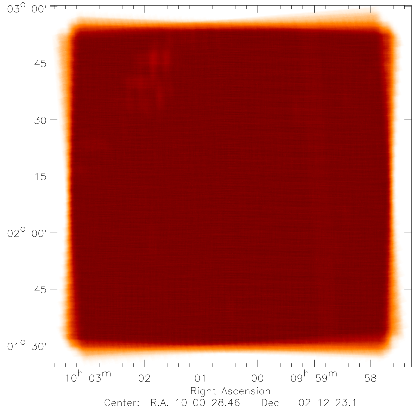
Figure 2: Actual 160 $\mu$m coverage map of the COSMOS field. Spots of reduced coverage near the top left of the map are due to dropping of data because of ‘speed bumps’ (see text).

Table 2 provides the key parameters of the actual PACS AOR implementations for each field. No significant source variability is expected for the dust-dominated emission of almost all detected sources. For this reason no timing contraints needed to be applied in the scheduling. For practical reasons scheduling of all AORs of a field during a visibility period was aimed for, and was typically but not always achieved. For fields near the plane of the ecliptic (COSMOS), asteroid passages may introduce another time dependent factor, as clearly demonstrated in mid-infrared detections during Spitzer observations of the COSMOS field (Sanders et al. sanders07 (2007)). The contrast between galaxies and asteroids is more favourable in the far-infrared. Still, bright asteroids would be detectable in individual maps if present but were not identified when differencing our individual COSMOS maps from a coaddition.

SPIRE maps for most of the PEP fields are obtained in coordinated observations by the HerMES key program (Oliver et al. oliver11 (2011)). For the two z$\sim$1 clusters we implemented within PEP simple 10′$\times$10′ ‘large’ SPIRE scanmaps in nominal scan speed, spatially dithering between five concatenated independent repetitions.

4 Data Analysis

4.1 Reduction of scanmap data and map creation

For scanning instruments with detectors that have a significant 1/f low frequency noise component, map creation usually follows one of two alternative routes. One is using full ‘inversion’ algorithms as widely applied by the cosmic microwave background community and the other uses highpass filtering of the detector timelines and subsequent direct projection, frequently used for Spitzer MIPS 70 or 160 $\mu$m reductions. An algorithm of the first ‘inversion’ type is available in the HCSS Herschel data processing in the form of an implementation and adaption to Herschel of a version of the MadMap code (Cantalupo et al. cantalupo10 (2010)). The alternative option that we adopt and describe in more detail below is using highpass filtering of the detector timelines and a direct ‘naive’ mapmaking. This choice is made because for our particular case of deep field observations, MadMap presently does not reach the same point source sensitivity, and the preservation of diffuse emission is not important for our science case. As noted, the cross-linked design of the PEP observations however does permit the future application of such inversion codes.

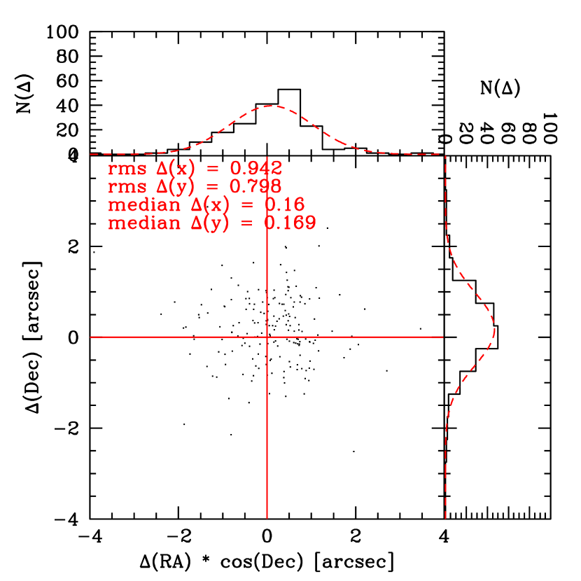
Figure 3: Offsets of GOODS-N 100 $\mu$m sources detected at $>5\sigma$ in a ‘blind’ extraction, compared to the corresponding 24 $\mu$m positions of the MIPS catalog used by Magnelli et al. (magnelli09 (2009)). A global offset has already been subtracted when deriving the PACS map.

Our reduction first proceeds on a per AOR level and is based on scanmap scripts for the PACS photometer pipeline (Wieprecht et al. wieprecht09 (2009)) in HCSS, with parameter settings and additions optimized for our science case. After retrieving PACS data and satellite pointing information we apply the first reduction steps to the time-ordered PACS data frames, identifying functional blocks in the data, flagging bad pixels, flagging any saturated data, converting detector signals from digital units to volts and the chopper position from digital units to physical angle.

After adding to the time-ordered data frames the instantaneous pointing obtained from the Herschel pointing product, we apply ‘recentering’ corrections. These are derived by comparing PACS maps obtained in a separate first processing of partial datablocks to deep 24 $\mu$m catalogs with accurate astrometry. Deep radio catalogs can also be used successfully. The corrections are derived by stacking at the positions of 24 $\mu$m sources a PACS 100 $\mu$m or 70 $\mu$m map that is obtained from typically about 15 minutes of data, and measuring the offset of the stacked PACS detection. The measured position offset is then corrected for this block of data in the original frames. The blocks used were typically restricted to one scan direction (all ‘odd’ or ‘even’ scanlegs of a map repetition, or subsets for the large COSMOS maps). By this procedure we correct for (1) the global offset pointing error of Herschel which is of order 2″ RMS and thus nonnegligible compared to PACS beamsizes, (2) differential pointing errors between different AORs that would lead to PSF smearing, in particular if AORs have been observed spread over long periods with different spacecraft orientations, (3) residual timing offsets between PACS data and pointing information that manifest themselves in small offsets between odd and even numbered scanlines and (4) pointing drifts over $\gtrsim$0.5 hour timescales within an AOR. Overall this leads to subarcsecond astrometry and reduces unnecessary PSF smearing by pointing effects. As a verification of this approach, Figure 3 compares the positions from a blind 100 $\mu$m catalog based on the final GOODS-N map with 24 $\mu$m positions.

Short glitches in the detector timelines caused by ionizing particle hits are flagged and interpolated with an HCSS implementation of the multi-resolution median transform, developed by Starck & Murtagh (starck98 (1998)) to detect faint sources in ISOCAM data. The different signatures of real sources and glitches in the pixel timeline at medium scan speed are discriminated by a multi-scale transform. This procedure is known to produce false detections on bright point sources. This was no problem for our deep field data except for a few bright COSMOS sources for which we locally reduced the glitch detection sensitivity.

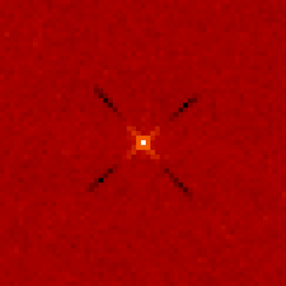
Figure 4: Correlation map extracted from GOODS-N 100 $\mu$m data, reflecting correlations induced by map projection and – in scan direction – by residual low frequency noise and highpass filtering. Correlations across the GOODS-N map are highly uniform and depend only on the relative $\Delta$x, $\Delta$y pixel positions, represented here with respect to the central pixel.

The ‘1/f’ noise of the PACS photometers, in fact roughly $\propto f^{-0.5}$ over the relevant frequencies, is removed by subtracting from each timeline the timeline filtered by a running box median filter of radius 15 samples (30″) at 70 $\mu$m or 100 $\mu$m and 26 samples (52″) at 160 $\mu$m. A mask is used to exclude sources from the median derivation. The mask is created by thresholding a S/N map produced from a smoothed coadded map that is including all AORs. Tests were done adding simulated sources to the timelines before masking and before highpass filtering. These tests were done on the real timelines of the full Lockman Hole AOR set for the red filter, thus implicitly including all real sky structures. They indicate that the filtering modifies the fluxes by less than 5% for masked point sources and $\sim$16% for very faint unmasked point sources. These results apply to ‘extragalactic deep field’ skies that are composed of many point sources and to our specific highpass filter setting. Extended sources need different filtering radii or reduction methods.

Flatfielding and flux calibration is done via the standard PACS pipeline calibration files. Because of the excellent in-flight stability of the photometer response, no use is made of the observations of the calibration sources internal to PACS that are obtained within each AOR. PEP science demonstration phase data were reduced using earlier versions of the responsivity calibration file and corrections derived on the stars $\gamma$Dra, $\alpha$Tau, and $\alpha$CMA; they are within 5% of the currently valid Version 5 of the reponsivity calibration file that has been validated over a wider set of flux calibration stars and asteroids.

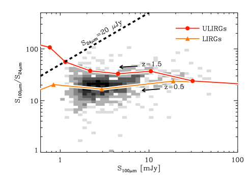
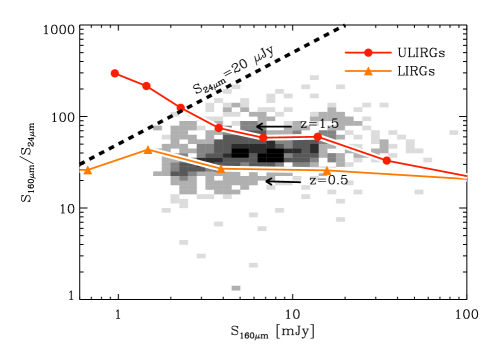
Figure 5: (Left) PACS 100 $\mu$m to MIPS 24 $\mu$m flux density ratio as a function of the PACS 100 $\mu$m prior catalog flux density. Shaded grey regions show the space density distribution of galaxies observed in the GOODS-S field. In that field, the MIPS 24 $\mu$m and PACS 100 $\mu$m catalogs reach at 3-$\sigma$ limit of 20 $\mu$Jy and 1.2 mJy, respectively. Red dots and orange triangles present the evolution with redshift of the PACS-to-MIPS flux density ratio of ultra-luminous (ULIRGs) and luminous (LIRGs) infrared galaxies, respectively, predicted using the Chary & Elbaz (chary01 (2001)) library. Each symbol corresponds to a given redshift, in intervals of $\Delta z=0.5$. On each track, we indicate on one point its corresponding redshift as well as as the path followed for increasing redshifts. The dashed black line represents the limit of the parameter space reachable using the MIPS 24 $\mu$m catalog available in this field; all the PACS 100 $\mu$m sources below this line would have a MIPS 24 $\mu$m counterpart in this catalog. (Right) PACS 160 $\mu$m to MIPS 24 $\mu$m flux density ratio as function of the PACS 160 $\mu$m flux density. Symbols and lines are the same as in the left panel.

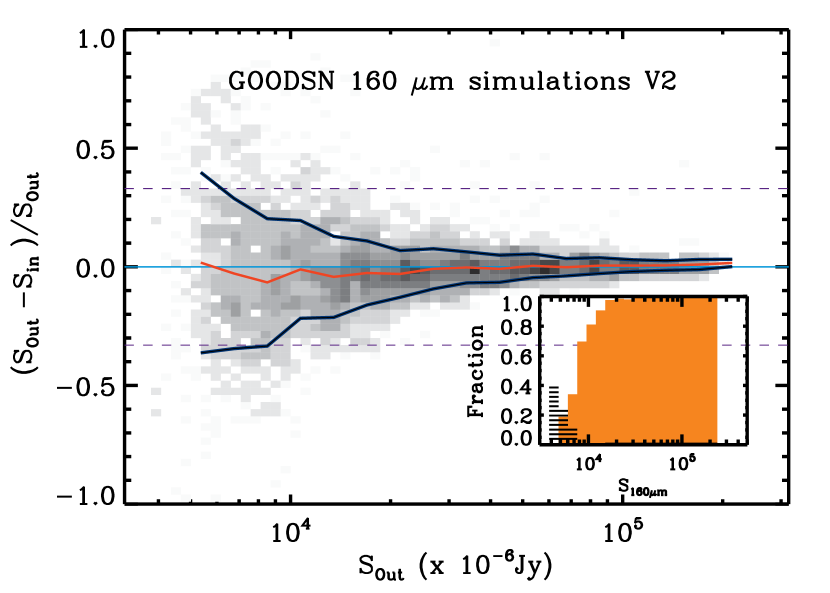
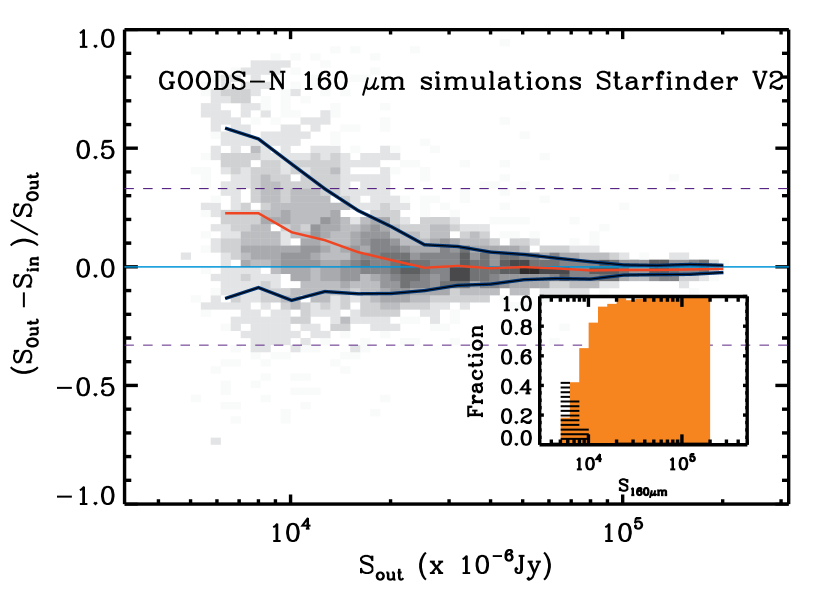
Figure 6: Results of artifical source addition experiments for the GOODS-N 160 $\mu$m extractions. Top: prior extraction, Bottom: blind extraction. The red lines represent the average photometric accuracy, blue lines set the standard deviation observed in each flux bin (after 3$\sigma$ clipping). The systematic boosting in the blind extraction is corrected in the final blind catalog. Given that, input and output fluxes are consistent with each other within a few percent, testifying that PACS fluxes are reliably extracted and retrieved by the adopted source extraction methods. The orange histogram represents the detection rate (or completeness) computed on the artificial injected sources, while black histograms denote cp the fraction of spurious sources as a function of output flux.

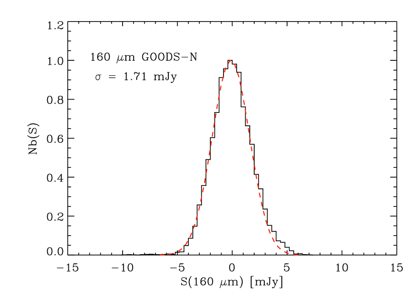
Figure 7: Noise estimate from randomly placing apertures on the GOODS-N 160 $\mu$m residual map.

Before creating maps from the timelines we discard various unsuitable parts of the data:

1. Observations of the internal calibration sources and a short subsequent interval during which the signal re-stabilizes. SDP observations had an erroneously large frequency of such calibration blocks.

2. Data taken during the turnaround loops between scans. The nominal pointing accuracy is not guaranteed during this phase, and highpass filtering effects on source flux are more severe if the telescope slows down strongly or even stops during a subtantial part of the filtering window.

3. Before a reduction of the star tracker operating temperature in Herschel operational day 320, ‘speed bumps’ in the satellite movement occured, when stars crossed irregularly behaving star tracker pixels. This led to an unkown mispointing. These events can be identified by comparing the two angular velocities obtained from (1) differentiating the positions on sky reported in subsequent entries of the pointing product and (2) the direct angular rate information in the pointing product.

4. Blue PACS bolometer data occasionally show fringes in the signal due to magnetic field interference that is heavily aliased into the timelines and final maps. Maps created separately for each individual scan line were visually inspected and scans clearly affected by fringing excluded from final mapping.

Maps are obtained from the timelines for each AOR via the HCSS ‘photProject’ projection algorithm, which is equivalent to a simplified version of the ‘drizzle’ method (Fruchter & Hook fruchter02 (2002)). Given the high data redundancy in the deep fields, PSF widths and noise correlation in the final map can be reduced choosing smaller projection drops than the physical PACS pixel size. Drop sizes between 1/8 and 1/4 of the physical PACS pixel size were used, depending on redundancy of the individual maps for each field. Weights of the different detectors in the projection consider the inverse variance derived from the noise in the dataset itself.

Maps from each AOR were coadded into final maps, weighting the indivudal maps by the effective exposure of each pixel. The final error map was computed as the standard deviation of the weighted mean. PSF fitting using the methods described in Sect. 4.2 assumes errors that are uncorrelated between neighbouring pixels. In practice, correlations exist due to projection and due to to the correlations that are caused by residual 1/f noise in the filtered timelines, in particular along the scan direction. We have verified that, because of the high redundancy of the data, these correlations are close to uniform across the final map, with less than 2% variation on the correction factor that is derived below. Thus we derived from PSF shape and correlation information a mean correlation correction factor which was then accounted for in the errors on the extracted fluxes. A correlation map is constructed, starting by collecting series of paired pixel values with same relative pixel coordinate offsets i,j. We take values $\Delta$f defined as the deviation in flux of a pixel in an individual AOR map from the corresponding pixel in the final map. This is a deviation from the mean with expectation value 0. Such values are taken for a large number of pairs in different positions in each AOR map and from different AORs. For each pixel-pairs series $\Delta$f_1,2, which corresponds to a specific i,j pixel offset, a correlation coefficient is calculated:

$$\rho(i,j)=\frac{\sum{\Delta f_{1}\Delta f_{2}}}{\sqrt{\sum{(\Delta f_{1})^{2}}}\sqrt{\sum{(\Delta f_{2})^{2}}}}$$ (1)

The correlation coefficients are stored as a map and written to the i,j position relative to the central pixel. Figure 4 shows an example correlation map. Normal error propagation for a weighted sum $g(x_{1}..x_{n})=\sum_{k=1}^{n}{a_{k}\cdot x_{k}}$, where the error are $\sigma_{k}$ and correlation coefficients $\rho(k,l)$ is:

$$\sigma_{g}^{2}=\displaystyle\sum_{k,l=1}^{n}{a_{k}\sigma_{k}\cdot a_{l}\sigma_{l}\cdot\rho(k,l)}$$ (2)

Given a PSF stamp with pixel values $P_{k}$ and a correlation between every two pixels $\rho(i,j)$ known from their relative position, the correlation correction factor to the derived errors is:

$$f^{2}=\frac{\displaystyle\sum\limits_{k}{P_{k}^{2}}}{\displaystyle\sum\limits_{i,j}{P_{i}P_{j}\rho(i,j)}}$$ (3)

$f$ is the ratio of the propagated error without correlations and the error calculated with the correlation terms. This assumes a near uniform error map on a scale of a PSF. For the typical pixel sizes (2″ and 3″ at 100 $\mu$m and 160 $\mu$m) and projection parameters used in the PEP SDP reductions, the corrections are about $f\approx 1.4$ for the 70 $\mu$m and 100 $\mu$m maps and $f\approx 1.6$ for the 160 $\mu$m maps.

Before availability of version 6 of the ArrayInstrument calfile that is containing the spatial transformation from PACS focal plane to sky, 160 $\mu$m data showed a $\approx$ 1″ spatial offset from 70 $\mu$m or 100 $\mu$m data. We corrected for this ad hoc in the 160 $\mu$m map fits headers, using offsets derived from a comparison of preliminary catalogs in the two bands.

4.2 Catalog creation

We extract source catalogs using point source fitting routines outside HCSS. We have used both blind extraction via the Starfinder PSF-fitting code (Diolaiti et al. diolaiti00 (2000)) and a guided extraction using 24 $\mu$m source priors, following the method described in Magnelli et al. (magnelli09 (2009)). We fitted with point spread functions extracted from the maps. Since these observed PSFs are limited in radius, we used for aperture corrections point spread functions obtained on Vesta. In order to match the observations, these were rotated to match the satellite position angle for each observation of a field, coadded and slightly convolved with a gaussian to match the actual FWHM of the combined map. For our reduction methods and projection into 2″ map pixels at 70 and 100 $\mu$m and 3″ at 160 $\mu$m, we have PSF FWHM for the 70, 100, and 160 $\mu$m maps of 6.46″, 7.39$\pm$0.10″, and 11.29$\pm$0.1″. The FWHM values are from gaussian fits to the core of the observed PSF. For the 100 and 160 $\mu$m widths we quote the error of the mean of measurements from five different fields.

All PEP blank fields benefit from extensive multi-wavelength coverage that is allowing guided extraction based on source positions at shorter wavelengths, where the depth and resolution of the observations are higher. This approach resolves most of the blending issues encountered in dense fields and allows straightforward multi-wavelength association (Magnelli et al. magnelli09 (2009), magnelli11 (2011); Roseboom et al. roseboom10 (2010)). However, to use this powerful method, prior source catalogs have to contain all the sources in the PACS images. Deep MIPS 24 $\mu$m observations, available for all our blank fields, should fulfill this criterion since they have higher resolution and are deeper than our current PACS observations. Moreover, since the 24 $\mu$m emission is strongly correlated with the far-infrared emission, those catalogs will not contain a large excess of sources without far-infrared counterparts. This largely avoids deblending far-infrared sources into several unrealistic counterparts, as could happen when using an optical prior catalog with very high source density. Figure 5 illustrates the validity of the MIPS 24 $\mu$m observations as PACS prior source positions.

At 100 $\mu$m, models and observations predict typical PACS-to-MIPS flux ratios in the range 5-50. A MIPS 24 $\mu$m catalog $50$ times deeper than the PACS observations is thus suited to perform guided source extraction. This is illustrated, for GOODS-S, in the left panel of Figure 5, where the observed PACS population lies well-below the boundary of the parameter space reachable by the MIPS 24 $\mu$m catalog. In all our blank fields, deep MIPS 24 $\mu$m catalogs fulfill this criterion (i.e., GOODS-S/N, COSMOS, LH, ECDFS, EGS…).

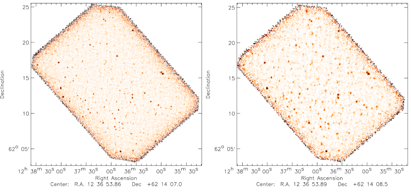
Figure 8: Science demonstration phase maps of the GOODS-N field. Left: 100 $\mu$m. Right: 160 $\mu$m

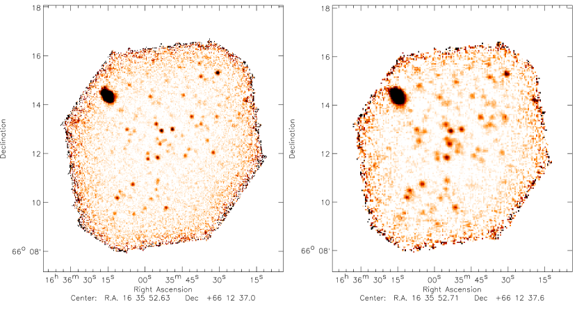
Figure 9: Science demonstration phase maps of the Abell 2218 lensing cluster field. Left: 100 $\mu$m. Right: 160 $\mu$m

At 160 $\mu$m, models and observations have typical PACS-to-MIPS flux ratios in the range 15-150. In all but one field, the deep MIPS 24 $\mu$m observations are at least 150 times deeper than our PACS observations; thus, they can be used as prior source positions. In GOODS-S, the deepest MIPS 24 $\mu$m observations are only 100 times deeper than our PACS observations. This limitation can be observed, in the right panel of Figure 5, as a slight truncation, at faint 160 $\mu$m flux density, of the high-end of the dispersion of the PACS-to-MIPS flux ratio. This truncation will introduce, at faint flux density, incompleteness in our prior catalog. However, we also observe that even at this faint 160 $\mu$m flux density, the bulk of the population has a PACS-to-MIPS flux ratio of $\thicksim 60$. The incompleteness introduced by the lack of MIPS 24 $\mu$m priors should thus be low or at least lower than the incompleteness introduced by source extraction methods at such low S/N. This was checked by comparing the GOODS-S 160 $\mu$m catalog obtained using blind source extraction with that obtained using guided source extraction: we find no significant difference, at faint 160 $\mu$m flux densities, in the number of sources in those two catalogs. In line with these finding, Magdis et al. (in prep) find very low fractions of 24$\mu$m undetected sources in very deep data from the GOODS-Herschel key program, $<2\%$ for ratios of detection limits S(100)/S(24)$>$43 and $<1\%$ for S(160)/S(24)$>$130.

Therefore, for all fields with deep MIPS 24 $\mu$m observations, we also extract source catalogs with a PSF-fitting method using 24 $\mu$m source positions as priors and following the method described in Magnelli et al. (magnelli09 (2009)). We used the same PSFs and aperture corrections as for the blind source extraction. Blind and prior catalogs were compared to verify the consistency between those two methods.

Completeness, fraction of spurious sources and flux reliability were estimated by running Monte Carlo simulations. Up to 10000 artificial sources were added to PACS science maps, and then extracted with the same techniques and configurations adopted for real source extraction. In order to avoid crowding, many such frames were created, each including a limited number of artificial sources. The number of frames and the number of sources added in each one depend on the size of the field under analysis and range between 20 and 500 sources (GOODS fields or COSMOS) per frame, repeated up to reaching the total of 10000. These synthetic sources cover a large range in flux, extending down to 0.5$\sigma$ ($\sigma$ being the measured rms noise in the PACS maps). The flux distribution follows the detected number counts, extrapolated to fainter level by means of the most successful fitting backward evolutionary model predictions (see Berta et al. berta11 (2011)). Sources are modelled using the Vesta PSF, manipulated as described above.

Figure 6 shows an example of results in the GOODS-N field at 160 $\mu$m. Completeness is defined here as the fraction of sources that have been detected with a photometric accuracy of at least 50% (Papovich et al. papovich04 (2004)). Spurious sources are defined as those extracted above 3$\sigma$ with an input flux lower than 3$\sigma$(Image). The systematic flux boosting in the blind extraction is corrected in the final blind catalog on the basis of these simulations.

Noise was estimated by extracting fluxes through 10000 apertures randomly positioned on residual maps. Figure 7 shows the distribution of the extracted fluxes, peaking around zero, as expected for a well subtracted background, and showing a Gaussian profile.

5 Science demonstration phase data

Figures 8 and 9 show the 100 $\mu$m and 160 $\mu$m maps of the GOODS-N and Abell 2218 fields as obtained during the Herschel science demonstration phase. A conservative threshold of 90% completeness is reached for the blind catalogs near 7 mJy and 15 mJy for 100 $\mu$m and 160 $\mu$m in the main parts of both GOODS-N and A2218. Above that level, the blind catalogs contain 153 and 126 sources for GOODS-N and 49 and 47 for Abell 2218, respectively. At the time of these observations, the Herschel scan maps were still exhibiting larger turnaround overheads than implemented later, and the PACS scanmap AOR had an unnecessarily large frequency of internal calibrations. Both these factors do not significantly affect the maps which are based on highpass-filtered reductions. With the exception of the overheads, these observations are representative for the results achievable in later mission periods during the observing times listed in Table 1, which reflect the later reduced overheads.

Figure 10: Comparison of blindly extracted and prior extracted 100 $\mu$m fluxes for the GOODS-N field.

Figure 10 compares 100 $\mu$m fluxes for the GOODS-N field between the blind (starfinder) extraction and extraction based on 24 $\mu$m priors. The blind detections have here been associated a posteriori to 24 $\mu$m sources, using a modification of the maximum likelihood method of Ciliegi et al. (ciliegi01 (2001)). The agreement is satisfactory with no systematic flux differences. Deviations occur at low fluxes where either catalog is incomplete and for few outliers where algorithms disagree in splitting a peak into two sources compared to one.

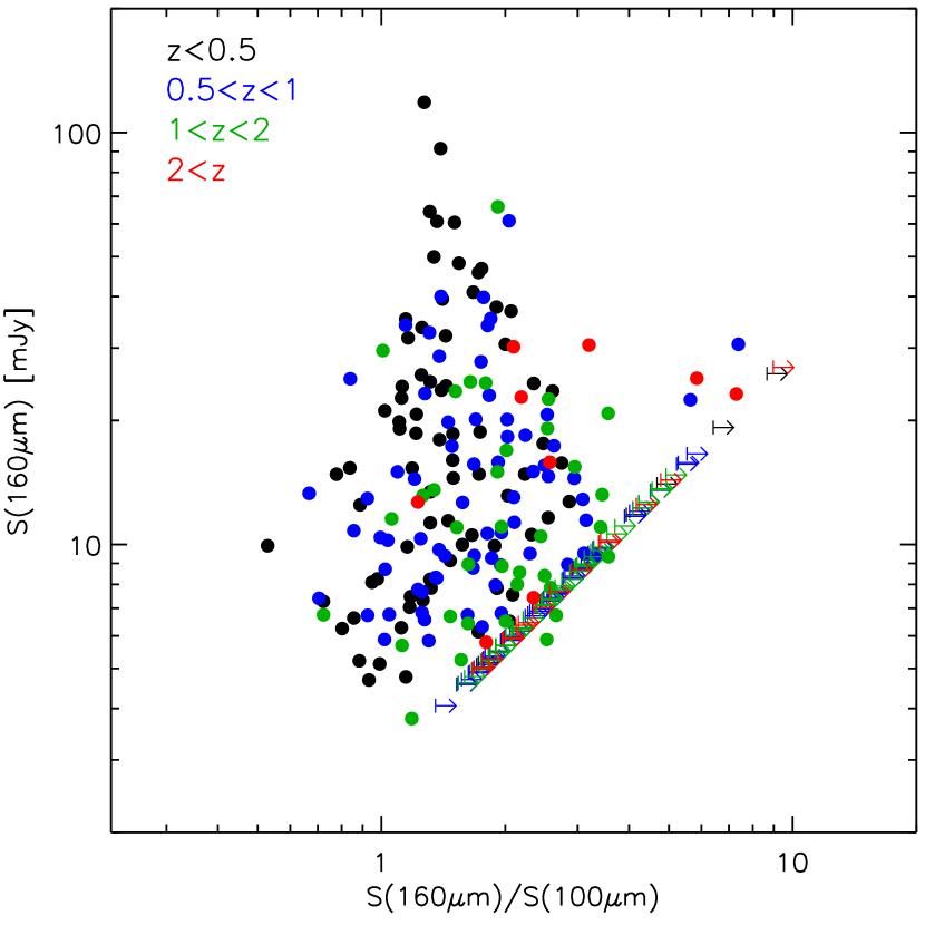
Figure 11: Color-magnitude diagram for 160 $\mu$m detected sources in the GOODS-N field

Figure 11 shows a ‘color-magnitude’ diagram for 160 $\mu$m detected sources in GOODS-N. As expected, there is a tendency for higher redshift sources to be redder in the 160/100 $\mu$m flux ratio, with considerable scatter due to measurement error and variation among the population. A detailed discussion of colors and SEDs is outside the scope of this work, see also Elbaz et al. (elbaz10 (2010)), Magnelli et al. (magnelli10 (2010)), Hwang et al. (hwang10 (2010)) and Dannerbauer et al. (dannerbauer10 (2010)) for first results on GOODS-N spectral energy distributions.

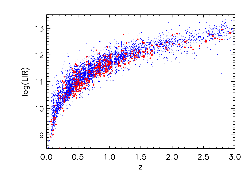
Figure 12: Red: Total infrared luminosity of GOODS-N sources detected above 3$\sigma$ in the PEP SDP data. Blue: Sources from the GOODS-S and COSMOS data illustrate the potential of the full PEP survey.

Figure 12 illustrates the potential of PEP to reach normal star forming galaxies up to redshifts z$\sim$2. The GOODS-N science demonstration phase data reach at z$\sim$2 infrared luminosities of 10¹²$L_{\odot}$ (star formation rates about 100 solar masses per year). The GOODS-N SDP observation thus reach the star formation ‘main sequence’ for massive galaxies at that redshift (Daddi et al. 2007a ). The GOODS-S data go deeper by a factor $\geq$2, and the COSMOS data provide the precious statistics at higher luminosities.

As an example of the PEP/PACS performance for deep surveys, the $>90\%$ completeness blind catalogs of the GOODSN and Abell 2218 SDP data will be released on the PEP website.

6 Overview of first science results of the PEP survey

6.1 The cosmic infrared background

One of the most imminent tasks of a large far-infrared space telescope is to resolve a large fraction of the cosmic infrared background into its constituent galaxies. The CIB peaks at roughly 150 $\mu$m (e.g. Dole et al. dole06 (2006)), making Herschel/PACS excellently suited to characterise the sources of its bulk energy output. Berta et al. (berta10 (2010)) used SDP observations of GOODS-N to derive 100 and 160 $\mu$m number counts down to 3.0 and 5.7 mJy, respectively. Altieri et al. (altieri10 (2010)) used strong lensing by the massive cluster Abell 2218 to push this limit down to 1 and 2 mJy, deeper by a factor $\sim$3 for both wavelengths. Berta et al. (berta11 (2011)) use a complement of PEP blank field observations including the deep GOODS-S observations to reach a similar depth as Altieri et al. but with the larger statistics provided by the blank field observations. They also add 70 $\mu$m counts overall reaching 1.1, 1.2, and 2.4mJy in the three PACS bands. To this depth, 58% (74%) of the COBE CIB as quoted by Dole et al. (dole06 (2006)) is resolved into individually detected sources at 100 (160 $\mu$m). These fractions reach 65% (89%) when including a P(D) analysis.

It is important to note that the direct COBE/DIRBE measurements have considerable uncertainties due to the difficulty of foreground subtraction. Similar to other wavelengths such as the $<$10keV X-rays (e.g. Brandt & Hasinger brandt06 (2006)) we are reaching the point where the lower limits to the cosmic background that are provided by the integral of the resolved Herschel measurements are more constraining than the direct measurements. Quoting ‘resolved fractions’ in reference to COBE hence starts to become problematic.

Because of the excellent multiwavelength coverage of the PEP fields, spectroscopic or photometric redshifts can be assigned to the detected sources, allowing us to determine the redshifts at which the CIB originates. To the depth reached by Berta et al. (berta11 (2011)), half of the resolved CIB originates at z$>$0.58, 0.67, 0.73 for wavelengths of 70, 100, and 160 $\mu$m, respectively. These redshifts are mild lower limits because they exclude faint sources that are not individually detected by Herschel, and naturally increase with wavelength, reflecting the dominant contributions by the far-infrared SED peak of increasingly distant objects.

Comparing the PEP counts and redshift distributions to backward evolutionary models tuned on pre-Herschel data, Berta et al. (berta11 (2011)) find for several models reasonable agreement with the total counts but more significant mismatches to the observed redshift distributions. Clearly, models have to be tuned in order to provide a satisfactory representation of the most recent data including Herschel.

The PEP GOODS-N SDP data have been used to derive first direct far-infrared based luminosity functions up to z$\sim$2–3 (Gruppioni et al. gruppioni10 (2010)). Strong evolution of the comoving infrared luminosity density (proportional to the star formation rate density) is found, increasing with redshift as $(1+z)^{3.8\pm 0.3}$ up to z$\sim$1. Global classification of the SEDs assigns to most objects either a starburst-like SED or an SED that is suggesting a modest AGN contribution.

6.2 ‘Calorimetric’ far-infrared star formation rates and star formation indicators

Star formation rates are one of the key measurables in galaxy evolution studies. ‘Calorimetric’ rest frame far-infrared measurements are the method of choice for massive and in particular dusty galaxies but have been out of reach for typical high-z galaxies in the pre-Herschel situation. Typically, star formation rates were measured from the rest frame ultraviolet, mid-infrared, submm/radio, or a combination of those methods. All of them require certain assumptions. Extracting a star formation rate from the rest frame ultraviolet continuum involves breaking the degeneracies between the star formation history and obscuration, and involves assumptions about the dust extinction law and/or geometry of the obscuring dust. Extrapolation from the mid-infrared or submm/radio requires the adoption of SED templates or assumptions that were derived locally but insufficiently tested at high redshift.

Nordon et al. (nordon10 (2010)) focussed on massive z$\sim$2 normal star forming galaxies that are currently the subject of intense study towards the role of secular and merging processes in their evolution (e.g. Förster Schreiber et al. foerster09 (2009)). They found ultraviolet-based star formation rates reasonably confirmed. At the rest frame optical bright end of these bright star forming galaxies, UV SFRs are overpredicting the calorimetric measurement by a factor 2 only. In contrast, a significant overprediction by a factor $\sim$4–7.5 was found when extrapolating from the 24 $\mu$m flux assuming that the local Universe Chary & Elbaz (chary01 (2001)) templates apply for the given mid-IR luminosity. This is in line with the encompassing SED studies of Elbaz et al. (elbaz10 (2010)) and Hwang et al. (hwang10 (2010)) which, combining PEP and HerMES as well as local Akari data, found that this overprediction by 24 $\mu$m extrapolation sets in at z$\sim$1.5, and that the FIR SED temperatures of high z galaxies are modestly colder than their local equivalents of similar total infrared luminosity.

There are two ways of looking at these results. Comparing at same total IR luminosity local galaxies with z$\sim$2 galaxies, the z$\sim$2 ‘overprediction’ when extrapolating from the mid-IR could either be due to an enhanced ratio of the PAH complex to the FIR peak, or due to a boosting of the mid-infrared emission via the continuum of a possibly obscured AGN (see also Papovich et al. papovich07 (2007) and Daddi et al. 2007b ). While most likely both factors are at work to some level, the setting in of the 24 $\mu$m overprediction at z$\sim$1.5 as well as Spitzer spectroscopy of mid-IR galaxies at these redshifts (Murphy et al. murphy09 (2009), Fadda et al. fadda10 (2010)) argues for a dominant role of stronger PAH. This is established by Nordon et al. nordon11 (2011) who show that z$\sim$2 GOODS-S galaxies with large 24 $\mu$m/FIR ratios indeed have PAH dominated spectra in the Fadda et al. (fadda10 (2010)) sample.

It is important to put this into the perspective of other properties of ${\rm L_{IR}}\sim 10^{12}L_{\odot}$ local and z$\sim$2 galaxies. Locally, such an object is a classical interacting or merging ‘ultraluminous infrared galaxy’ (ULIRG, Sanders & Mirabel sanders96 (1996)) with star formation concentrated in a few hundred parsec sized region. Such star formation rates are well above the local ‘main sequence’ (Brinchmann et al. brinchmann04 (2004)). At z$\sim$2, objects with the same star formation rates can be on the main sequence (Daddi et al. 2007a ) and are often not interacting/merging but massive, turbulent disks with star formation spread out over several kpc (e.g. Genzel et al. genzel08 (2008), Shapiro et al. shapiro08 (2008), Förster Schreiber et al. foerster09 (2009)). It is hence not surprising that SED templates calibrated on local compact mergers fail to reproduce the more extended star formation at z$\sim$2. The locally defined connotations of the ‘ULIRG’ term, beyond its basic definition by IR luminosity, obviously do not apply automatically at high redshift.

Rodighiero et al. (rodighiero10 (2010)) use the direct Herschel far-infrared star formation rates in the PEP GOODS-N field to characterize the evolution of the Specific Star Formation Rate (SSFR)/mass relation up to z$\sim$2. They find a steepening from an almost flat local relation to a slope of -0.5 at z$\sim$2.

Concerning the most highly star forming high redshift objects, Magnelli et al. (magnelli10 (2010)) combine the GOODS-N and Abell 2218 PACS data with submm surveys. They use PACS to sample the Wien side of the far-infrared SED of submm galaxies and optically faint radio galaxies with accurately known redshifts. The directly measured dust temperatures and infrared luminosities are in good agreement with estimates that are based on radio and submm data and are adopting the local universe radio/far-infrared correlation (see also the dedicated PEP/HerMES test of the high-z radio/far-infrared correlation by Ivison et al. (ivison10 (2010)). This confirmation of huge O(1000$M_{\odot}$yr^-1) star formation rates for SMGs is in support of a predominantly merger nature of SMGs, since such star formation rates are very hard to sustain with secular processes (e.g. Davé et al. dave10 (2010)).

6.3 The role of environment

PEP data cover a wide range of environments. As first steps, Magliocchetti et al. (magliocchetti11 (2011)) derive correlation functions and comoving correlation lengths at z$\sim$1 and 2 from the GOODS-S data which also provide evidence for most infrared bright z$\sim$2 galaxies in this field residing in a filamentary structure. At z$\sim$1, Popesso et al. (popesso11 (2011)) observe a reversal of the local star formation rate - density relation which is linked to the presence of AGN hosts that are favoring high stellar masses, dense regions and high star formation rates.

6.4 Studies of individual galaxy populations

Dannerbauer et al. (dannerbauer10 (2010)) use the $\lesssim 10\arcsec$ beam PEP maps to verify the identifications of (sub)millimeter galaxies and test the potential of PACS colors and mid-infrared to radio photometric redshifts for these objects. Santini et al. (santini10 (2010)) use the Herschel points to break the degeneracy between dust temperature and dust mass that is inherent to submm-only data, and derive high dust masses for a sample of submillimeter galaxies. Comparison of these high dust masses with the relatively low gas phase metallicities either implies incompletely understood dust properties or a layered structure which is combining low metallicity visible outer regions with a highly obscured interior.

Magdis et al. (magdis10 (2010)) use a stacked detection of z$\sim$3 Lyman break galaxies to constrain their far-infrared properties. Similar to the SMG/OFRG study of Magnelli et al. (magnelli10 (2010)), this work highlights the selection effects in the luminosity / dust temperature plane that are imposed by groundbased submm detection. Bongiovanni et al. (bongiovanni10 (2010)) study Lyman $\alpha$ emitters in the GOODS-N field. PACS detections of part of these galaxies are evidence for overlap with the dusty high redshift galaxy population.

6.5 AGN-host coevolution: Two modes?

Within the complex task of disentangling the coevolution of AGN and their host galaxies, and the role of AGN feedback, rest frame far-infrared observations provide a unique opportunity to determine host star formation rates. This rests on the assumption that the host dominates over the AGN in the rest frame far-infrared. This assumption is motivated by determinations of the intrinsic SED of the AGN proper, which is found to drop towards the far-infrared (e.g. Netzer et al. netzer07 (2007), Mullaney et al. mullaney11 (2011)). Compared to previous attempts from the submm (e.g. Lutz et al. lutz10 (2010)) and Spitzer (e.g. Mullaney et al. mullaney10 (2010)), Herschel performance provides a big step forward. Shao et al. (shao10 (2010)) use the PEP GOODS-N observations and the Chandra Deep Field North to map out the host star formation of AGN of different redshift and AGN luminosity. The host far-infrared luminosity of AGN with ${\rm L_{2-10keV}}\approx 10^{43}{\rm erg\,s}^{-1}$ increases with redshift by an order of magnitude from z=0 to z$\sim$1, similar to the increase with redshift in star formation rate of inactive massive galaxies. In contrast, there is little dependence of far-infrared luminosity on AGN luminosity, for ${\rm L_{2-10keV}}\lesssim 10^{44}{\rm erg\,s}^{-1}$ AGN at z$\gtrsim$1. In conjunction with properties of local and luminous high-z AGN, this suggests an interplay between two paths of AGN/host coevolution. A correlation of AGN luminosity and host star formation for luminous AGN reflects an evolutionary connection, likely via merging. For lower AGN luminosities, star formation is similar to that in non-active massive galaxies and shows little dependence on AGN luminosity. The level of this secular, non-merger driven star formation increasingly dominates over the correlation at increasing redshift.

7 Conclusions

Deep Herschel far-infrared surveys are a powerful new tool for the study of galaxy evolution and for unraveling the constituents of the cosmic infrared background. We have described here the motivation, field selection, observing strategy and data analysis for the PEP guaranteed time survey. Science demonstration phase data of GOODS-N and Abell 2218 are discussed to illustrate the performance of Herschel-PACS for this science. The wide range of initial science results from the PEP data is briefly reviewed.

- (1) Altieri, B., Berta, S., Lutz, D., et al., 2010, A&A, 518, L17
- (2) Aussel, H., Cesarsky, C.J., Elbaz, D., Starck, J.L. 1999, A&A, 342, 313
- (3) Berta, S., Magnelli, B., Lutz, D., et al., 2010, A&A, 518, L30
- (4) Berta, S., et al., 2011, A&A, in press
- (5) Bongiovanni, A., Oteo, I., Cepa, J., et al., 2010, A&A, 519, L4
- (6) Brandt, W.N., Hasinger, G., 2006, ARA&A, 43, 827
- (7) Brinchmann, J., Charlot, S., White, S.D.M., et al. 2004, MNRAS, 351, 1151
- (8) Cantalupo, C.M., Borill, J.D., Jaffe, A.H., Kisner, T.S., Stompor, R., 2010, ApJS, 187, 212
- (9) Chary, R., Elbaz, D., 2001, ApJ, 556, 562
- (10) Ciliegi, P., Gruppioni, C., McMahon, R., Rowan-Robinson, M., 2001, Ap&SS, 276, 957
- (11) Daddi, E., Dickinson, M., Morrison, G., et al. 2007, ApJ, 670, 156
- (12) Daddi, E., Alexander, D.M., Dickinson, M., et al. 2007, ApJ, 670, 173
- (13) Dannerbauer, H., Daddi, E., Morrison, G.E., et al. 2010, ApJ, 720, L144
- (14) Davé, R., Finlator, K., Oppenheimer, B.D., et al., 2010, MNRAS, 404, 1355
- (15) Davis, M., Guhathakurta, P., Konidaris, N. P., et al. 2007, ApJ, 660, L1
- (16) Diolaiti, E., Bendinelli, O., Bonaccini, D., et al. 2000, A&AS, 147, 335
- (17) Dole, H., Rieke, G.H., Lagache, G., et al., 2004, ApJS, 154, 93
- (18) Dole, H., Lagache, G., Puget, J.-L., et al., 2006, A&A, 451, 417
- (19) Eales, S., Dunne, L., Clements, D., et al. 2010, PASP, 122, 499
- (20) Ebeling, H., Jones, L.R., Perlman, E., et al., 2000, ApJ, 543, 133
- (21) Egami, E., Rex, M., Rawle, T.D., et al. 2010, A&A, 518, L12
- (22) Elbaz, D., Hwang, H.S., Magnelli, B., et al., 2010, A&A, 518, L29
- (23) Elbaz, D., et al. 2011, A&A, submitted (arXiv 1105.2537)
- (24) Fadda, D., Yan, L., Lagache, G., et al., 2010, ApJ, 719, 425
- (25) Förster Schreiber, N.M., Genzel, R., Bouché, N., et al., 2009, ApJ, 706, 1364
- (26) Fruchter, A. S. & Hook, R. N. 2002, PASP, 114, 144
- (27) Genzel, R., Cesarsky, C., 2000, ARA&A, 38, 761
- (28) Genzel, R., Burkert, A., Bouché, N., et al. 2008, ApJ, 687, 59
- (29) Griffin, M., Abergel, A., Abreu, A., et al. 2010, A&A, 518, L3
- (30) Gruppioni, C., Pozzi, F., Andreani, P., et al. 2010, A&A, 518, L27
- (31) Hasinger, G., Altieri, B., Arnaud, M., et al. 2001, A&A, 365, L45
- (32) Hauser, M.G., Arendt, R.G., Kelsall, T., et al., 1998, ApJ, 508, 25
- (33) Hopkins, A.M., Beacom, J.F., 2006, ApJ, 651, 142
- (34) Hughes, D.H., Serjeant, S., Dunlop, J., et al., 1998, Nature393, 241
- (35) Hwang, H.S., Elbaz, D., Magdis, G., et al., 2010, MNRAS, 409, 75
- (36) Ivison, R.J., Magnelli, B., Ibar, E., et al., 2010, A&A, 518, L31
- (37) Kiss, Cs., Ábrahám, P., Klaas, U., et al. 2001, A&A, 399, 177
- (38) Le Floc’h, E., Papovich, C., Dole, H., et al. 2005, AJ, 632, 169
- (39) Lehmer, B.D., Brandt, W.N., Alexander, D.M., et al., 2005, ApJS, 161, 21
- (40) Lilly, S.J, Le Fevre, O., Hammer, F., Crampton, D. 1996, ApJ. 460, L1
- (41) Lutz, D., Mainieri, V., Rafferty, D., et al., 2010, ApJ, 712, 1287
- (42) Madau, P., Ferguson, H.C., Dickinson, M.E., et al. 1996, MNRAS, 283, 1388
- (43) Magdis, G., Elbaz, D., Hwang, H.S., et al., 2010, ApJ, 720, L185
- (44) Magliocchetti, M., Santini, P., Rodighiero, P., et al., 2011, MNRAS, in press (arXiv:1105.4093)
- (45) Magnelli, B., Elbaz, D., Chary, R. R., et al. 2009, A&A, 496, 57
- (46) Magnelli, B., Lutz, D., Berta, S., et al., 2010, A&A, 518, L28
- (47) Magnelli, B., Elbaz, D., Chary, R.R., et al. 2011, A&A, 528, 35
- (48) Mullaney, J.R., Alexander, D.M., Huynh, M., Goulding, A., Frayer, D., 2010, MNRAS, 401, 995
- (49) Mullaney, J.R., Alexander, D.M., Goulding, A.D., Hickox, R.C., 2011, MNRAS, in press (arXiv:1102.1425)
- (50) Murphy, E.J., Chary, R.-R., Alexander, D.M., et al., 2009, ApJ, 698, 1380
- (51) Netzer, H., Lutz, D., Schweitzer, M., et al. 2007, ApJ, 666, 806
- (52) Nordon, R., Lutz, D., Shao, L., et al., 2010, A&A, 518, L24
- (53) Nordon, R., Lutz, D., Berta, S., et al., 2011, ApJ, submitted (arXiv:1106.1186)
- (54) Oliver, S., et al., 2011, MNRAS, submitted
- (55) Papovich, C., Dole, H., Egami, E., et al., 2004, ApJS, 154, 70
- (56) Papovich, C., Rudnick, G., Le Floc’h, e., et al., 2007, ApJ, 668, 45
- (57) Pilbratt, G., Riedinger, J.R., Passvogel, T., et al. 2010, A&A, 518, L1
- (58) Poglitsch, A., Waelkens, C., Geis, N., et al. 2010, A&A, 518, L2
- (59) Popesso, P., Rodighiero, G., Saintonge, A., et al., 2011, A&A, in press (arXiv:1104.1094)
- (60) Puget, J.-L., Abergel, A., Bernard, J.-P., et al., 1996, A&A, 308, L5
- (61) Rodighiero, G., Cimatti, A., Gruppioni, C., et al., 2010, A&A, 518, L25
- (62) Roseboom, I.G., Oliver, S., Kunz, M., et al., 2010, MNRAS, 409, 48
- (63) Rowan-Robinson, M., 2001, ApJ, 549, 745
- (64) Sanders, D.B., Mirabel, I.F., 1996, ARA&A, 34, 749
- (65) Sanders,D.B., et al. 2007, ApJS, 172, 86
- (66) Santini, P., Maiolino, R., Magnelli, B., et al. 2010, A&A, 518, L154
- (67) Scoville, N., Aussel, H., Brusa, M., et al. 2007, ApJS, 172, 1
- (68) Shao, L., Lutz, D., Nordon, R., et al., 2010, A&A, 518, L26
- (69) Shapiro, K.L., Genzel, R., Förster Schreiber, N.M., et al., 2008, ApJ, 682, 231
- (70) Soifer, B.T., Helou, G., Werner, M. 2008, ARA&A, 46, 201
- (71) Starck, J. & Murtagh, F. 1998,PASP, 110, 193
- (72) Tran, K.H., Kelson, D.D., van Dokkum, P., et al., 1999, ApJ, 522, 39
- (73) Wieprecht, E., et al. 2009, ADASS XVIII, eds. D. Bohlender, D. Durand and P. Dowler, ASP Conference Series 411, 531