Surrejoinder to the Comment on:
“Thermostatistics of Overdamped Motion of Interacting Particles”
by Y. Levin and R. Pakter.

I Initial considerations

The example investigated in Ref. andradeprl10 corresponds to a system of interacting vortices undergoing an overdamped motion, whose dynamical behavior is studied through a molecular dynamics procedure and the corresponding results, at the stationary state, are shown to be in perfect agreement with the solution of a nonlinear Fokker-Planck equation for $T=0$ as well as for finite values of $T$.

In their Rejoinder levin2 Levin and Pakter repeat some of the points raised in their previous Comment levin1 (already refuted in our first Reply reply1 ) and raise some new ones concerning our recent publication andradeprl10 . The present queries are refuted in this Surrejoinder, whenever relevant for the results of Ref. andradeprl10 . It should be mentioned that in both Comment levin1 and Rejoinder levin2 , one finds incorrect statements, as well as a clear lack of knowledge about important advances in the area related to Ref. andradeprl10 . In what follows, we highlight some misleading points found in Refs. levin2 ; levin1 .

(a) In Ref. levin1 the authors analyze the case $T=0$, and treat the system by replacing the interactions acting on a given particle by a potential, showing that this potential satisfies an inhomogeneous Helmholtz equation. By solving such an equation, the authors claim to have obtained an exact solution for this problem. Clearly, this is a misleading statement, since the authors have used a mean-field type of approximation to obtain the differential equation that led to their solution. This point has already been refuted, as can be seen on item (5) of our Reply reply1 , and we reinforce it herein. Unfortunately, the authors can not understand this fundamental restriction of their solution.

(b) In both Refs. levin2 and levin1 by Levin and Pakter, one can notice very clearly that these authors did not read Ref. andradeprl10 carefully. Our theory, like all other theories, has its validity subjected to some conditions. One of the most important conditions for this theory concerns the fact that the two-particles density may be approximated by the product of two one-particle densities, i.e., $\rho^{(2)}(x,x\prime,t)\approx\rho(x,t)\rho(x\prime,t)$. All counter-examples shown in Refs. levin1 ; levin2 violate this basic requirement, clearly written in our Letter andradeprl10 . It is not surprising that the the results obtained by these authors are in contrast with ours. In this Surrejoinder, we show an example of this, when we consider a particular counter-example used in the Rejoinder by Levin and Pakter levin2 , namely, the potential $\exp(-x^{4})$, and simulate it satisfying our conditions: the result is exactly what was predicted by our theory. We can only regret that such a hasty reading of our paper has led to a waste of (important) time of many scientists. We are not willing to spend more time in explaining again what is already clearly written in our paper.

(c) The fact that the system is described by Newton’s laws does not necessarily imply that one should have a Boltzmann-Gibbs statistical mechanics; the authors seem to ignore this very basic point.

(d) In both Comments levin1 ; levin2 , the authors show to be unaware of the vast literature developed in the last 15 years, concerning nonlinear Fokker-Planck equations and their relation to generalized entropies (different from the Boltzmann-Gibbs one); many of these references are cited in Ref. andradeprl10 . In the same way that the linear Fokker-Planck equation may be related to the Boltzmann-Gibbs entropy, as shown in standard statistical-mechanics textbooks, one can also show that nonlinear Fokker-Planck equations may be related to generalized entropies. The authors also do not seem to understand this important point.

II Two different physical situations

Consider the problem of a fixed amount of fluid confined to a flat-bottom cylindrical container. Assuming that the fluid is incompressible, simple hydrostatics says that the potential energy $U_{h}$ of such system is given by

$$U_{h}=\frac{\rho_{h}g}{2}\int{dxdy~{}z^{2}},$$ (1)

where $\rho_{h}$ is the density of the fluid, $g$ is the gravity, and $z(x,y)$ is the height of the column of fluid over a certain point. If energy if dissipated, the system should evolve towards the minimum potential energy, with a constant $z$ along the container. This seems quite obvious, but a specialist in liquids may present good evidence to contest all these observations. A simple look inside a narrow glass container filled with some fluid shows us the presence of a meniscus. Such specialist could even solve exactly the shape of the meniscus for a particular liquid and conclude that Eq. (1) is wrong as well as all conclusions derived from it. However, a narrow container is an unfair situation. In a wide container, Eq. (1) works perfectly at any point, but very close to the edge of the container. The specialist in liquids could also point out that his/her approach works better as it solves $z$ at any point of the system, far or close to the edge. However, this approach is more specific rather than more general, since the shape of the meniscus is highly dependent on the nature of the liquid and container, while Eq. (1) will work efficiently to any container, as long as it is not so narrow, filled with any incompressible fluid.

In this contribution we will show that the effects observed by Levin and Pakter levin2 ; levin1 , in the same way as a meniscus in a confined fluid, are negligible effects that are amplified in highly confined regimes. In the same way as the hydrostatic example mentioned above, one can solve this system, taking care of all microscopic details of the particular interaction, and find the whole profile, bulk and edge. We choose, however, a more general approach to this problem, that describes the correct way the particles distribute themselves in the bulk system. As we show in our Letter andradeprl10 , our approach works for systems where the particles spread over a region that is large, when compared with the typical interaction range over the particles. Moreover, our approach is more general than Levin and Pakter solution levin1 as it is NOT dependent on the particular interaction.

III Physical argumentation in favor of Tsallis entropy as a maximum for the system under investigation

In our Letter andradeprl10 , we have concluded that, under certain conditions, systems of interacting over-damped particles evolve to a state that maximizes Tsallis entropy with $\nu=2$. Contrary to what Levin and Pakter believe, this conclusion is not that surprising but can be demonstrated quite simply. The present derivation is a little less rigorous than the one we introduce in Ref. andradeprl10 , but easier to comprehend, and may help us to make our point.

Let us assume that one can obtain the potential energy of a system of interacting particles $U_{s}$ in the form,

$$U_{s}=\int{dxdy~{}u(x,y)},$$ (2)

where $u(x,y)$ is the density of potential energy. To determine $u$ we will use the simplifying assumption that the density of particles is continuous and constant. In this case we can identify $u(x,y)=\rho(x,y)U_{1}(\rho)$, where $\rho$ is the number of particles per unity of area, and $U_{1}(\rho)$ is the potential energy of a single particle due to the interaction with its neighbors. Under the assumption that $\rho$ is continuous and constant, we have,

$$U_{1}=\rho\int{dr^{2}U(r)}=a\rho,$$ (3)

where $a\equiv\int{dr^{2}U(r)}$, and $U(r)$ is a radially symmetrical interacting potential. Including the energy due to an external potential, $U_{e}$, we obtain,

$$U_{s}=\int{dxdy(a\rho+U_{e})\rho}.$$ (4)

We now consider that energy is dissipated until the system evolves towards the minimum energy. As we explain in our Letter andradeprl10 , the term in $\rho^{2}$ in Eq. (4) is identified with the negative of the Tsallis entropy with index $\nu=2$. Therefore such system evolves towards the maximum Tsallis entropy.

Clearly this method is valid only when some conditions are met. Firstly, we assume that $\rho$ is a continuous function that varies slowly within the interaction range of a particle. Precisely, in the derivation presented in Ref. andradeprl10 , we assume that, within the interaction range of the particles, we have $\rho(r)=\rho_{0}+\nabla\rho\cdot\mathbf{r}$, that is, we neglect terms of second order in the variation of the density profile, and assume that $\rho$ varies linearly within the interaction range. The inclusion into Eq. (4) of the external potential $U_{e}$ also imposes that it varies slowly with the interaction range. Situations where such condition do not hold include, but are not limited to, abrupt changes in the external potential.

As we explicitly stated in our Letter andradeprl10 , our approach is not adequate when $\rho$ in not locally homogeneous, for instance, hard-core potentials or potentials with an attractive part should induce local fluctuations that can not be considered in our method. Anther condition where it fails is with long-range potentials, where the interaction range is not defined. Also, if $\rho$ goes to zero at some point of the system, one can not assume the linear variation beyond this point, as a negative density has no meaning. This indicates that effects observed close to this point are not accounted for by our method. However, these effects are microscopic, in the sense that they vanish for distances a few units away of the interaction range.

To object to our method, Levin and Pakter considered systems with interaction range of some arbitrary length $\lambda$, and present results for particles confined to a region of only a few units of $\lambda$ (see the horizontal axis of Fig. 1 of their Comment levin1 and Fig. 2 of their Rejoinder levin2 ). As already mentioned, our method does not account for effects close to the edge of the profile, and since Levin and Pakter confine the particles to the extreme, these edge effects appear rather amplified in their results. In our Reply reply1 , we asked why Levin and Pakter decided to present results for this extreme case rather than in the conditions we considered and effectively studied (in their notation, this would be achieved by simply making $q^{2}N=800$). In this condition, the particles spread over a region more than a $100\lambda$ wide and edges effects become negligible. In Fig. 1 here we used their analytical solution to demonstrate that the effect they expect is indeed negligible for a less confined system. We ask now Levin and Pakter to stop diverging the subject. Do they admit that the blue curve of Fig. 1 is their analytical solution? Do they admit that any deviation of our solution is an edge effect that becomes negligible when the particles spread over several units of the interaction range $\lambda$? If they do not admit these statements, what are their evidences for the contrary? If they do admit it, why didn’t they write it clearly in their Comment levin1 ?

IV Reply to Levin and Pakter’s Rejoinder levin2

1) Levin and Pakter claim that the thermodynamic limit can be obtained only in the two ways: (a) by scaling the vortex charge to leave it proportional to $\sqrt{N}$; and (b) by rescaling the confining potential strength at the same time the number of particles grows, $\alpha\sim N$.

This statement is nothing but false. What Levin and Pakter appear not to know, but it is well explained in any introductory text on statistical mechanics, is that one obtains the thermodynamic limit by increasing the number of particles, while leaving the intensive properties of the system unchanged. For instance, think of $N$ particles confined in a box of volume $V$. To obtain the thermodynamic limit, one should scale both $V$ and $N$, keeping the average density $N/V$ constant. The outlandish scaling proposed by Levin and Pakter does not keep constant the density of particles that, in the asymptotic limit of this scaling, diverges to infinity. Therefore, although this scaling may result in a invariant form for $\rho/N$, it is not the correct way to obtain the thermodynamic limit. To Levin and Pakter benefit, we explain here how one should proceed to obtain the thermodynamic limit in a system like ours. In the same way as in the box mentioned previously, one should simply scale the dimension $L_{y}$ linearly with $N$, in order to keep $N/L_{y}$ constant. We invite Levin and Pakter to verify that in this way, different from their scaling, both the density profile and the average energy per particle do not diverge, but remain invariant with $N$.

2) Levin and Parker state that a differential equation for the particle density only makes sense in the limit where $N\to\infty$.

We agree. As we explained in item (1), it is possible to obtain this limit in a simple and straightforward way. For some reason, this escaped Levin and Pakter comprehension.

3) Levin and Pakter state that “even allowing the incorrect coarse-graining procedure of Andrade et al., (…) the density distribution will not be given by a q-exponential” since a q-exponential is a smooth function and can not explain the discontinuity observed in the edge of the density function. Moreover, Levin and Pakter state that this discontinuity is observed in our results.

If present, this discontinuity is surely not a relevant effect in the regime investigated by us, that is, less confined systems where particles spread over several units of the interaction range $\lambda$. In our first Reply reply1 to their Comment levin1 , we included in the inset of Fig. 1 (for clarity, repeated in Fig. 1 of this Surrejoinder) the solution proposed by Levin and Pakter for the conditions we studied. It became already clear from these results how negligible, if present, this effect would be in this regime. Regarding the numerical results presented in their Rejoinder levin2 , since they do not provide details of their simulations, we can not fathom what Levin and Pakter did wrong in their simulations, or even if they are really integrating the correct equations of motion [see Eq. (9) of our Letter]. Considering the evident asymmetry and non-smooth aspect of the curve presented in Fig. 1 of their Rejoinder levin2 , we can only guess that they did not perform an average over enough realizations. In any event, we now show in Fig. 1 of the present Surrejoinder our numerical solution along with their numerical and analytical solutions for the regime with $q^{2}N=800$, that reproduces the regime we investigate. As one can see, although there is a good agreement between our and their numerical solution, the analytical derivation does not follow the observed profile. We can, however, use Levin and Pakter’s qualitative solution at this regime to demonstrate that the discontinuity, if present, is negligible at the regime where the particles are not so confined.

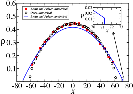
Figure 1: Numerical results for the density profile obtained from numerical simulations. We used the same conditions as Fig. 1 of our Letter andradeprl10 , namely, $N=800$, $\alpha=10^{-3}f_{0}/\lambda$, and $L_{y}=20\lambda$. The black circles and red squares correspond to the numerical simulation reported in Ref. andradeprl10 and in the Rejoinder by Levin and Pakter levin2 , respectively, while the straight blue line corresponds to the solution according to Eq. (3) from Levin and Pakter’s Comment levin1 . Clearly their solution is not compatible with the concavity of the density profile obtained from our molecular dynamics simulations. The inset shows that the discontinuity in their solution is barely noticeable for these physical conditions.

4) Levin and Pakter ask “for exactly what value of $N$ do the authors expect that Tsallis entropy will start determining the particle distribution at T=0?”

If Levin and Pakter had read our Letter with attention, they would know by now that as few as $800$ particles are enough to observe a distribution that follows our predictions and maximizes Tsallis entropy.

5) Levin and Pakter state that we do not provide “any reason or indication why they believe that the standard Boltzmann-Gibbs statistical mechanics will not apply to the system studied by them.”

We do not question that other approaches using BG statistics could be applied to solve the problem we have investigated. We are sure, however, that if correctly applied, these approaches should corroborate our results. Maybe Levin and Pakter still do not understand our results. In our approach, all the particle-particle interactions of the system are included into the Tsallis entropic term with $\nu=2$. For the case with $T>0$, this means that we map the problem of a non-ideal gas of particles into an ideal gas with an entropy that caries both BG and Tsallis contributions. The usefulness of our approach is that it can be generalized to a wide range of interaction potentials. By contrast, in order to treat the same problem only with BG statistics, one would need to include the particular interaction, which requires the solution to be specific for each type of interaction potential.

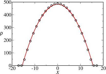
Figure 2: Numerical results for the density profile obtained from numerical simulations of a one-dimensional system and the interaction potential proposed in the Rejoinder by Levin and Pakter levin2 , namely, $U(x)=f_{0}\exp{[-(x/\lambda)^{4}]}/2$. This potential approaches a square-barrier, being rather difficult to simulate through standard molecular dynamics techniques. In order to obtain minimum energy configurations, we coupled a steepest-descent Monte Carlo algorithm. The system has $N=10000$ particles confined by an external potential with intensity $\alpha=3.0f_{0}/\lambda$. The solid line corresponds to the theoretical prediction Eq. (14) of our Letter andradeprl10 with $a=0.75$. As depicted, when the particles spread over several units of $\lambda$, we observe a parabolic profile. This is in perfect agreement with our theoretical model.

6) Levin and Pater state that from “Eq. (1) used by Andrade is derived the unlucky Eq. (13) of their PRL”, and that this equation leads to the conclusion that the stationary state for particles interacting by any short-range force is always parabolic. Levin and Pakter also present numerical results indicating that this result is not true for a potential given by $U(x)\sim e^{-x^{4}}$.

First, Levin and Pakter should note that we do NOT deduce Eq. (13) from Eq. (1), but from the equations of motion for the particles, Eq. (9) of the Letter andradeprl10 . Equation (13), however, is equivalent to the nonlinear Fokker-Plank equation, Eq. (5), that, as we show, drives the system towards the state that maximizes Tsallis entropy. Second, we invite Levin and Pakter to investigate this system in the conditions we know our method to be valid, that is, a system with a less intense confining potential, where particles spread over several units of the interaction range of the potential, instead of only four. We believe that had they followed these guidelines, by now they would know that this results in a parabolic density profile, as shown in Fig. 2. In short, as long as a few conditions are fulfilled, a wide family of short-range repulsive interaction potentials can be modeled by Eq. (13) of our Letter andradeprl10 .

7) Levin and Pakter claim that the velocity distribution follows Maxwell-Boltzmann.

We did not study velocity distributions in Ref. andradeprl10 , although this is an interesting property which deserves a careful analysis on its own. Herein, we notice again, as in many other parts of their Comments levin2 ; levin1 , that they state as ours, assumptions that we have never made. Could they indicate any allusions made in Ref. andradeprl10 concerning velocity distributions? This is not the best way to carry a fair scientific discussion.

8) Levin and Pakter state that our system “has nothing to do with Tsallis statistics.”

We believe that we have demonstrated that the system do evolve to the state of maximum Tsallis entropy. We are sorry that Levin and Pakter neither present any evidence of the contrary nor believe in our results.

V Final considerations

It is our understanding that, in their two Comments levin2 ; levin1 , Levin and Pakter did not give any relevant contributions to the problem addressed in Ref. andradeprl10 . Their arguments are, most of the times misleading. In our two replies, we have refuted their criticisms in full detail. We thus consider the present discussion as closed.

References

- (1) J. S. Andrade, Jr., G. F. T. da Silva, A. A. Moreira, F. D. Nobre, and E. M. F. Curado, Phys. Rev. Lett. 105, 260601 (2010).
- (2) Y. Levin and R. Pakter, arXiv:1105.1316v1 (2011).
- (3) Y. Levin and R. Pakter, arXiv:1104.0697v1 (2011).
- (4) J. S. Andrade, Jr., G. F. T. da Silva, A. A. Moreira, F. D. Nobre, and E. M. F. Curado, arXiv:1104.5036v1 (2011).