Geometric scaling behavior of the scattering amplitude for DIS with nuclei

Abstract:

The main question, that we answer in this paper, is whether the initial condition can influence on the geometric scaling behavior of the amplitude for DIS at high energy. We re-write the non-linear Balitsky-Kovchegov equation in the form which is useful for treating the interaction with nuclei. Using the simplified BFKL kernel, we find the analytical solution to this equation with the initial condition given by the McLerran-Venugopalan formula. This solution does not show the geometric scaling behavior of the amplitude deeply in the saturation region. On the other hand, the BFKL Pomeron calculus with the initial condition at $x_{A}=1/mR_{A}$ given by the solution to Balitsky-Kovchegov equation, leads to the geometric scaling behavior. The McLerran - Venugopalan formula is the natural initial condition for the Color Glass Condensate (CGC) approach. Therefore, our result gives a possibility to check experimentally which approach: CGC or BFKL Pomeron calculus, is more adequate.

1 Introduction.

Geometric scaling behavior of the scattering amplitude is one of the most qualitative and well founded features of the high energy scattering in the framework of the CGC approach. In the saturation domain it follows from the general structure of the non-linear equation (see Ref.[1]) that governs the scattering amplitude in high density QCD [2, 3, 4, 5, 6, 7]. In the vicinity of the saturation scale the geometric scaling behavior was derived [8] from the linear evolution [14, 9]. The geometric scaling behavior means that the amplitude turns out to be a function of one dimensionless variable: $\tau=r^{2}Q^{2}_{s}\left(x;b\right)$ instead of three variables: $x$ - the fraction of the energy carried by the parton interacting with the virtual photon in DIS, $r$- the typical size of the interacting dipole ($r\propto 1/Q$ where $Q$ is the photon virtuality), and $b$ is the impact parameter of the scattering process. Actually, the geometric scaling behavior reflects that the only dimensional parameter , that governs the scattering process in the saturation domain, is the saturation scale $Q_{s}$ and $\tau$ is just the only dimensionless variable that we can construct. Implicitly, such a behavior assumes that the amplitude in the saturation region does not depend on the initial condition for the non-linear equation. As we have mentioned this idea looks consistent with the geometric scaling behavior of the scattering amplitude in the perturbative QCD region near to the saturation scale [8].

However, it has been noticed in Ref. [10] that the geometric scaling behavior of the scattering amplitude cannot be correct for the DIS with nuclei if the McLerran-Venugopalan formula [4] is used as the initial condition for this process. This initial condition itself shows the saturation behavior on the scale which is the saturation scale at low energy ($Q_{s}\left(x=x_{0};b\right)$). Generally , this behavior could be different from the geometric scaling one as it is shown in Ref. [10].

In this paper we revisit this problem and we try to answer the following questions:(i) could the initial condition affect the behavior of the scattering amplitude at $\tau\,\gg\,1$; (ii) can we trust the McLerran-Venugopalan formula deeply in the saturation region; and (iii) what initial condition we need to use to reproduce the geometric scaling behavior.

We believe that all these questions are needed to be answered not only due to pure theoretical interest but also because the geometric scaling behavior is seen experimentally both for hadron and nucleus scattering (see Refs.[11]).

2 General solution to the simplified non-linear equation.

The nonlinear Balitsky-Kovchegov equation for the scattering amplitude of the dipole with size $r$ has the following form[6, 7]:

$$\frac{\partial N\left(r,Y;b\right)}{\partial\,Y}\,\,\, = \,\,\frac{C_{F}\,\alpha_{S}}{2\,\pi^{2}}\,\,\int\,d^{2}r^{\prime}\,K\left(r;r^{\prime}\right)\times\Big{\{}2N\left(r^{\prime},Y;\vec{b}\,-\,\frac{1}{2}\,(\vec{r}-\vec{r}\>^{\prime})\right)\,\,$$

$$- \,\,N\left(r,Y;\vec{b}\right)\,\,-\,\,N\left(r^{\prime},Y;\vec{b}-\frac{1}{2}\,(\vec{r}-\vec{r}\>^{\prime})\right)\,N\left(\vec{r}-\vec{r}\>^{\prime},Y;b-\frac{1}{2}\vec{r}\>^{\prime}\right)\Big{\}}$$

where $Y=\ln(1/x)$ is the rapidity of the incoming dipole; $N$ is the imaginary part of the scattering amplitude and $b$ is the impact parameter of this scattering process. $\alpha_{S}$ is the QCD coupling, below we will use the following notation $\bar{\alpha}_{S}=\alpha_{S}N_{c}/\pi$. The BFKL kernel $K\left(r;r^{\prime}\right)$ has the following form

$$K\left(r;r^{\prime}\right)\,\,=\,\,\frac{r^{2}}{(\vec{r}\,-\,\vec{r}\>^{\prime})^{2}\,r^{\prime 2}}\,$$ (2.2)

2.1 Simplified equation for scattering with nuclei

Considering the interaction of the dipole with a nucleus we can simplify this equation. Indeed, neglecting the non-linear term in Eq. (2) we have the linear BFKL equation and the amplitude for dipole-nucleus scattering can be written as

$$N^{BFKL}_{A}=\int d^{2}b^{\prime}\,N^{BFKL}_{N}\left(r,\,Y;\,\vec{b}\,-\,\vec{b}^{\prime}\right)\,T_{A}(b^{\prime})=T_{A}(b)\,\int d^{2}b"\,N_{N}(r,Y;\,b")\,=\,N_{N}\left(r,Y;t=0\right)T_{A}(b)$$ (2.3)

where $\vec{b}\,-\,\vec{b}^{\prime}\,\equiv\,\vec{b}"$ and $T_{A}(b)$ is the number of the nucleons at given impact parameter $b$ in the nucleus. It can be calculated as the following integral

$$T_{A}(b)\,\,=\,\,\int^{+\infty}_{-\infty}dz\,\rho\left(b,z\right)$$ (2.4)

where $\rho$ is the density of the nucleons in a nucleus and $z$ is the longitudinal coordinate of the nucleon. This number depends on $b$ but it is of the order of $A^{1/3}$.

In Eq. (2.3) we assumed that $|\vec{b}-\vec{b}^{\prime}|\leq R_{N}\,\ll\,b^{\prime}\approx R_{A}$. One can recognize that this is typical Glauber-type assumption which holds for interaction with nuclei if the energy is not so high that the radius dipole-nucleon interaction can be considered as much smaller than the nucleus radius. $N_{N}\left(r,Y;t=0\right)$ is the imaginary part of dipole-nucleon amplitude at momentum transfer $t=0$, which proportional to dipole-nucleon total cross section.

Let us solve Eq. (2) using Eq. (2.3) as the first iteration. One can see that the second iteration leads to the following expression

$$\frac{\partial N^{(2)}_{A}\left(r,Y;t=0\right)}{\partial\,Y}\,\,\, = \,\,\frac{\bar{\alpha}_{S}}{2\,\pi}\,\int\,\frac{d^{2}r^{\prime}\,r^{2}}{(\vec{r}\,-\,\vec{r}\>^{\prime})^{2}\,r^{\prime 2}}\,\times\Big{\{}2\,T_{A}(b)\,N^{BFKL}_{N}\left(r^{\prime},Y;t=0)\right)\,$$

$$- \,\,T_{A}(b)\,N^{BFKL}_{N}\left(r,Y;t=0\right)\,\,-\,\,T^{2}_{A}(b)\,N^{BFKL}_{N}\left(r^{\prime},Y;t=0)\right)\,N^{BFKL}_{N}\left(\vec{r}-\vec{r}\>^{\prime},Y;t=0\right)\Big{\}}$$

Introducing $N^{eff}_{N}=N_{A}/T(b)$ one can see that Eq. (2.1) can be viewed as the first iteration of the equation

$$\frac{\partial N^{eff}_{N}\left(r,Y;t=0\right)}{\partial\,Y}\,\,\, = \,\,\frac{\bar{\alpha}_{S}}{2\,\pi}\,\int\,\frac{d^{2}r^{\prime}\,r^{2}}{(\vec{r}\,-\,\vec{r}\>^{\prime})^{2}\,r^{\prime 2}}\,\times\Big{\{}2\,N^{eff}_{N}\left(r^{\prime},Y;t=0)\right)\,$$

$$- \,\,N^{eff}_{N}\left(r,Y;t=0\right)\,\,-\,\,T_{A}(b)\,N^{eff}_{N}\left(r^{\prime},Y;t=0)\right)\,N^{eff}_{N}\left(\vec{r}-\vec{r}\>^{\prime},Y;t=0\right)\Big{\}}$$

The non-linear equation in the form of Eq. (2.1) was firstly proposed in Refs. [2, 3] and it is valid for energies at which the radius of dipole - nucleon interaction is much smaller than the nucleus radius. The energy dependence of radius of dipole - nucleon interaction unfortunately cannot be solved in the framework of the Balitsky-Kovchegov non-linear equation of Eq. (2) (see Ref.[12]) since it demands some additional input from the non-perturbative QCD. The high energy phenomenology based on the soft Pomeron approach leads to

$$R^{2}\left(\mbox{dipole - nucleon}\right)\,=\,\,R^{2}_{0}+\alpha^{\prime}_{P}(0)\,Y\,\,\ll\,\,R^{2}_{A}$$ (2.7)

in wide range of rapidity $Y$ including the LHC energies for $R^{2}_{0}=10\,GeV^{-2}$ and $\alpha^{\prime}_{P}(0)\leq 0.2\,GeV^{-2}$.

2.2 Simplified BFKL kernel

The BFKL kernel of Eq. (2.2) is rather complicated and the analytical solution with this kernel has not been found. In Ref.[13] it was suggested to simplify the kernel by taking into account only log contributions. From formal point of view this simplification means that we consider only leading twist contribution to the BFKL kernel. Notice that the kernel of Eq. (2.2) includes all twists contributions. We are dealing with two kinds of logs in Eq. (2), which corresponds two different kinematic regions: $\tau\,<\,1$ and $\tau\,>\,1$.

2.2.1 $\tau\,<\,1$

In this kinematic region we can simplify $K\left(r;r^{\prime}\right)$ in Eq. (2) in the following way[13], since $r^{\prime}\gg r$ and $|\vec{r}-\vec{r}^{\prime}|>r$

$$\int d^{2}r^{\prime}\,K\left(r,r^{\prime}\right)\,\,\rightarrow\,\pi\,r^{2}\,\int^{\frac{1}{\Lambda^{2}_{QCD}}}_{r^{2}}\frac{dr^{\prime 2}}{r^{\prime 4}}$$ (2.8)

Introducing $n^{eff}_{N}\left(r,Y;t=0\right)=N^{eff}_{N}\left(r,Y;t=0\right)/r^{2}$ we obtain

$$\frac{\partial^{2}n^{eff}_{N}\left(r,Y;t=0\right)}{\partial Y\,\partial\ln\left(1/(r^{2}\Lambda^{2}_{QCD})\right)}\,\,\,=\,\,\frac{\bar{\alpha}_{S}}{2}\,\Big{(}2n^{eff}_{N}\left(r,Y;t=0\right)\,\,-\,\,r^{2}\Lambda^{2}_{QCD}\,T_{A}(b)\,\left(n^{eff}_{N}\right)^{2}\left(r,Y;t=0\right)\Big{)}$$ (2.9)

One can see that the simplified kernel of Eq. (2.8) sums $\Big{(}\bar{\alpha}_{S}\ln\left(r^{2}\,\Lambda^{2}_{QCD}\right)\Big{)}^{n}$.

2.2.2 $\tau\,>\,1$

The main contribution in this kinematic region originates from the decay of the large size dipole into one small size dipole and one large size dipole. However, the size of the small dipole is still larger than $1/Q_{s}$. This observation can be translated in the following form of the kernel

$$\int d^{2}r^{\prime}\,K\left(r,r^{\prime}\right)\,\,\rightarrow\,\pi\,\int^{r^{2}}_{1/Q^{2}_{s}(Y,b)}\frac{dr^{\prime 2}}{r^{\prime 2}}\,\,+\,\,\pi\,\int^{r^{2}}_{1/Q^{2}_{s}(Y,b)}\frac{d|\vec{r}-\vec{r}^{\prime}|^{2}}{|\vec{r}-\vec{r}^{\prime}|^{2}}$$ (2.10)

One can see that this kernel leads to the $\ln\left(r^{2}Q^{2}_{s}\right)$-contribution. Introducing a new function $\tilde{N}^{eff}_{N}\left(r,Y;t=0\right)\,\,=\,\,\int^{r^{2}}dr^{2}\,N^{eff}_{N}\left(r,Y;t=0\right)/r^{2}$ one obtain the following equation

$$\frac{\partial^{2}\tilde{N}^{eff}_{N}\left(r,Y;t=0\right)}{\partial Y\,\partial\ln r^{2}}\,\,=\,\,\bar{\alpha}_{S}\,\left\{\left(1\,\,-\,T_{A}\left(b\right)\,\frac{\partial\tilde{N}^{eff}_{N}\left(r,Y;t=0\right)}{\partial\ln r^{2}}\right)\,\tilde{N}^{eff}_{N}\left(r,Y;t=0\right)\right\}$$ (2.11)

The Mellin transform of the full BFKL kernel of Eq. (2.2) has the form

$$\chi\left(\gamma\right)\,\,=\,\,\int\frac{d\xi}{2\pi i}\,e^{-\gamma\xi}\,K\left(r;r^{\prime}\right)\,\,=\,\,2\psi(1)\,-\,\psi(\gamma)\,-\,\psi(1-\gamma)$$ (2.12)

where $\xi\,=\,\ln(r^{2}/r^{\prime 2})$ and $\psi(z)=d\ln\Gamma(z)/dz$ with $\Gamma(z)$ equal to Euler gamma function. The simplified kernel replaces Eq. (2.12) by the following expression

$$\chi\left(\gamma\right)\,\,=\,\,\left\{\begin{array}[]{l}\,\,\,\frac{1}{\gamma}\,\,\,\,\,\mbox{for}\,\,\,\tau\geq\,1\,;\\ \\ \,\,\,\frac{1}{1\,-\,\gamma}\,\,\,\,\,\mbox{for}\,\,\,\tau\,\leq\,1\,;\end{array}\right.$$ (2.16)

One can see that the advantage of the simplified kernel of Eq. (2.16) is that it provides a matching with the DGLAP evolution equation[14] in Double Log Approximation (DLA) for $\tau<1$. We will show below that this kernel leads to the geometric scaling behavior of the scattering amplitude. The other attempt[15] to use a simplified kernel is related to the BFKL kernel in the diffusion approximation,namely,

$$\chi(\gamma)\,\,=\,\,\omega_{0}\,\,+D\,\left(\gamma-\frac{1}{2}\right)^{2}\,\,+\,\,{\cal O}\left(\left(\gamma-\frac{1}{2}\right)^{3}\right)$$ (2.17)

with

$$\omega_{0}\,\,=\,\,4\,\bar{\alpha}_{S}\ln 2\,;\,\,\,\,\,\,\,\,\,D\,\,=\,\,14\bar{\alpha}_{S}\zeta(3)$$ (2.18)

In this approach we loose any matching with the GLAP evolution. Both simplified kernels reproduce the geometric scaling behavior giving the illustrations to the general conclusions of Ref.[1].

2.3 Traveling wave solution and the geometric scaling behavior of the scattering amplitude.

It is well known (see Refs.[2, 1, 15, 16]) that the equation for the saturation scale does not depend on the particular form of the non-linear term in Eq. (2) and it has the form

$$\ln\left(Q^{2}_{s}(Y)/Q^{2}(Y=Y_{0})\right)\,\,=\,\,\frac{\chi\left(\gamma_{cr}\right)}{1-\gamma_{cr}}\,\Big{(}Y\,\,-\,\,Y_{0}\Big{)}$$ (2.19)

with the critical anomalous dimension $\gamma_{cr}$ given by

$$-\frac{\partial\omega(\gamma_{cr})}{\partial\gamma_{cr}}\,\,=\,\,\frac{\omega(\gamma_{cr})}{1-\gamma_{cr}}$$ (2.20)

Inserting Eq. (2.12) in Eq. (2.20) one obtains

$$\gamma_{cr}\,\,=\,\,\frac{1}{2}\;\;\;\;\mbox{and}\;\;\;\;\ln\left(Q^{2}_{s}(Y)/Q^{2}(Y=Y_{0})\right)\,\,=\,\,4\bar{\alpha}_{S}\left(Y-Y_{0}\right)$$ (2.21)

In the vicinity of the saturation scale $\tau\to 1$ the behavior of the dipole amplitude has the form [16, 8]

$$N\left(Y;r\right)\,\,\propto\left(r^{2}Q^{2}_{s}\right)^{1-\gamma_{cr}}$$ (2.22)

We illustrate this behavior approaching to the saturation scale from the perturbative QCD region ($\tau\ll 1$). In this region we can use Eq. (2.9) neglecting the non-linear term. This equation has a simple DLA solution

$$n^{eff}_{N}\,\,=\,\,\exp\Big{(}2\sqrt{\bar{\alpha}_{S}\,\left(Y-Y_{0}\right)\,\ln\left(r^{2}\,Q^{2}_{s}\left(Y=Y_{0}\right)\right)}\Big{)}$$ (2.23)

which leads to the following expression for dipole -nucleus amplitude (see Eq. (2.3))

$$N_{A}\,\, = \,\,T_{A}\left(b\right)\,\exp\Big{(}2\sqrt{\bar{\alpha}_{S}\left(Y-Y_{0}\right)\,\ln\left(1/\left(r^{2}\,Q^{2}_{s}\left(Y=Y_{0}\right)\right)\right)}\,+\,\ln\left(r^{2}\,\,Q^{2}_{s}\left(Y=Y_{0}\right)\right)\Big{)}\,$$ (2.24)

$$\xrightarrow{\tau\to 1} \,T_{A}\left(b\right)\,\left(r^{2}Q^{2}_{s}\right)^{1/2}\,\exp\Big{(}-\frac{\ln^{2}\tau}{8\ln\left(Q^{2}_{s}\left(Y\right)/Q^{2}_{s}\left(Y=Y_{0}\right)\right)}\Big{)}$$

Therefore, in vicinity of the saturation scale if $\ln\tau\ll\sqrt{8\ln\left(Q^{2}_{s}\left(Y\right)/Q^{2}_{s}\left(Y=Y_{0}\right)\right)}$ the dipole-nucleus amplitude can be written as

$$N_{A}\,\,=\,\,T_{A}\left(b\right)\,\phi_{0}\,\left(r^{2}Q^{2}_{s}\right)^{1/2}\,\,=\,\,\phi_{0}e^{\frac{1}{2}z}$$ (2.25)

where

$$z\,\,=\,\,4\,\bar{\alpha}_{S}\left(Y-Y_{0}\right)\,+\,\ln\left(r^{2}Q^{2}_{s}\left(A;Y=Y_{0}\right)\right)\,\,=\,\,\xi_{s}\,\,+\,\xi$$ (2.26)

where

$$\xi_{s}\,=\,\ln\Big{(}Q^{2}_{s}\left(A;Y\right)/Q^{2}_{s}\left(A;Y=Y_{0}\right)\Big{)}\,=\,4\bar{\alpha}_{S}\left(Y-Y_{0}\right),\;\;\;\;\mbox{and}\;\;\;\xi\,=\,\ln\Big{(}r^{2}Q^{2}_{s}\left(A;Y=Y_{0}\right)\Big{)}$$ (2.27)

The saturation scale for nucleus we defined as $Q_{s}^{2}\left(A,Y=Y_{0}\right)\,\,=\,\,T^{2}_{A}\left(b\right)\,Q_{s}\left(N;Y=Y_{0}\right)$ where $Q_{s}\left(N;Y=Y_{0}\right)$ is the saturation scale for the nucleon at the initial energy. $\phi_{0}$ is a constant that absorbers all pre-exponential factors in the DLA solution. It is instructive to notice that $\phi_{0}\propto\bar{\alpha}_{S}$[2, 13].

Inside the saturation region we are looking for the solution of Eq. (2.11) in the form[13, 10]:

$$\widetilde{N}^{eff}_{N}\,\,=\,\,T^{-1}_{A}(b)\int^{\xi}_{\xi_{s}}d\xi^{\prime}\,\Big{(}1\,-\,e^{-\phi(\xi^{\prime},Y)}\Big{)}$$ (2.28)

From Eq. (2.28) one can see that we can easily to calculate the dipole-nucleus amplitude

$$N_{A}\,\,=\,\,T_{A}\left(b\right)N^{eff}_{N}\,\,=\,\,1\,\,-\,\,e^{-\phi\left(\xi,Y\right)}$$ (2.29)

Substituting Eq. (2.28) into Eq. (2.11) we obtain

$$\phi^{\prime}_{Y}\,e^{-\phi}\,\,=\,\,\bar{\alpha}_{S}\widetilde{N}^{eff}_{N}\,e^{-\phi}$$ (2.30)

Canceling $e^{-\phi}$ and differentiating with respect to $\xi$ we obtain the equation in the form:

$$\frac{\partial^{2}\phi}{\partial Y\,\partial\xi}\,\,=\,\,\,\bar{\alpha}_{S}\,\Big{(}1\,-\,e^{-\phi\left(Y;\xi\right)}\Big{)}$$ (2.31)

Using variable $\xi_{s}$ and $\xi$ we can rewrite Eq. (2.30) in the form

$$\frac{\partial^{2}\phi}{\partial\xi_{s}\,\partial\xi}\,\,=\,\,\frac{1}{4}\Big{(}1\,-\,e^{-\phi\left(Y;\xi\right)}\Big{)}$$ (2.32)

or in the form of

$$\frac{\partial^{2}\phi}{\partial z^{2}}\,\,-\,\,\frac{\partial^{2}\phi}{\partial x^{2}}\,\,=\,\,\frac{1}{4}\Big{(}1\,-\,e^{-\phi\left(Y;\xi\right)}\Big{)}$$ (2.33)

for $z$ defined in Eq. (2.26) and $x=\,\xi_{s}-\xi$.

Eq. (2.33) has general traveling wave solution (see Ref.[17] formula 3.4.1)

$$\int^{\phi}_{\phi_{0}}\frac{d\phi^{\prime}}{\sqrt{c\,+\,\frac{1}{2(\lambda^{2}-\kappa^{2})}\Big{(}\phi^{\prime}-1+e^{-\phi^{\prime}}\Big{)}}}\,\,=\,\,\kappa\,x+\lambda\,z$$ (2.34)

where $c,\phi_{0},\lambda$ and $\kappa$ are arbitrary constants that should be found from the initial and boundary conditions.

From the matching with the perturbative QCD region (see Eq. (2.25)) we have the following initial conditions:

$$\phi\left(t\equiv z=0,x\right)\,\,=\,\,\phi_{0}\,;\,\,\,\,\,\,\phi^{\prime}_{z}\left(t\equiv z=0,x\right)\,\,=\,\,\frac{1}{2}\,\phi_{0}$$ (2.35)

These conditions allow us to find that $\kappa=0$ and $c=0$ for $\phi_{0}\,\ll\,1$. Therefore, solution of Eq. (2.34) leads to the geometric scaling since it depends only on one variable: $z$.  It has the form[13]

$$\sqrt{2}\int^{\phi}_{\phi_{0}}\frac{d\phi^{\prime}}{\sqrt{\phi^{\prime}-1+e^{-\phi^{\prime}}}}\,\,=\,\,z$$ (2.36)

For arbitrary $\phi_{0}$ the solution has the form

$$\int^{\phi}_{\phi_{0}}\frac{d\phi^{\prime}}{\sqrt{\frac{1}{4}\,\phi_{0}^{2}\,+\,\frac{1}{2}\Big{(}\phi^{\prime}\,-\,\phi_{0}\,+\,e^{-\phi^{\prime}}\,-\,e^{-\phi_{0}}\Big{)}}}\,\,=\,\,z$$ (2.37)

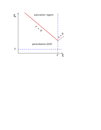
Figure 1: Saturation region: $z=\xi_{s}+\xi$ and $x=\xi_{s}-\xi$ for interaction with dilute target (proton)

Solution of Eq. (2.36) we can use in the case of interaction of the dipole with rather dilute target. In this case the initial conditions are determined by perturbative QCD and have the form of Eq. (2.35).

One can see that if $\phi_{0}\propto\bar{\alpha}_{S}\,\ll\,1$ the solution of Eq. (2.36) gives

$$\phi\,\,=\,\,\phi_{0}e^{\frac{1}{2}z}$$ (2.38)

while at $z\gg 1$ Eq. (2.36) leads to

$$\phi\,\,=\,\,\frac{z^{2}}{8}$$ (2.39)

3 Dipole-nucleus amplitude: solution for one critical line and violation of the geometric scaling behavior.

The main ingredient of Color Glass Condensate (CGC) approach is the assumption that there exists such value of energy that we can describe dipole-nucleus amplitude using the McLerran-Venugopalan formula[4]:

$$N_{A}\left(r^{2};Y;b\right)\,\,\,=\,\,1\,\,-\,\,\exp\Big{(}-\bar{\alpha}_{S}^{2}\,Const\,r^{2}ln\left(r^{2}Q^{2}_{s}(Y=Y_{0})\right)\Big{)}\,\,=\,\,1-\exp\Big{(}-r^{2}\,Q^{2}_{s}\left(A;Y=Y_{0}\right)\Big{)}$$ (3.40)

The last equation is a simplification of the original formula but it reflects the main physics of saturation and considerable simplify calculations.

Eq. (3.40) can be translated into the boundary conditions for $\phi$ on the line $Y=Y_{0}$ ($\xi_{s}=0$, see Fig. 3) that has the following form:

$$\phi\left(\xi_{s}=0;\xi\right)\,\,=\,\,\phi_{0}e^{\xi}$$ (3.41)

while solution of Eq. (2.36) gives quite a different function at $\xi_{s}$ = 0 (see Fig. 2). Therefore we need to find a more general solution than it is given by Eq. (2.34).

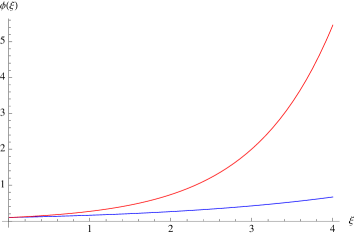
Figure 2: Boundary conditions at Y=$Y_{0}$. The red(upper) line is $\phi(\xi)$ from McLerran-Venugopalan formula while the blue (lower) one is the solution of Eq. (2.36).

One of the general features of solution of Eq. (2.36) is the increase of $\phi$ in the saturation region. it means that only in the vicinity of the critical line we have to keep term $\exp\left(-\phi\right)$. Inside of the saturation region we can neglect this term reducing the equation to the simple one, namely,

$$\phi_{\xi_{s},\xi}\,\,=\,\,\frac{1}{4};\,\,\,\,\,\mbox{or}\,\,\,\,\,\,\frac{\partial^{2}\phi}{\partial t^{2}}\,\,-\,\,\frac{\partial^{2}\phi}{\partial x^{2}}\,\,=\,\,\frac{1}{4}$$ (3.42)

with the initial and boundary conditions of Eq. (2.35) and Eq. (3.41), respectively.

It is well known that the solution of this equation is different for $t=z<x\;(\xi<0)$ and $t=z>x\;(\xi>0)$[17]. For $t=z<x\;(\xi<0)$ the solution is not affected by the boundary conditions and it has the form

$$\phi_{1}\left(z\right)\,\,=\,\,\frac{1}{8}z^{2}\,\,+\,\,\frac{\phi_{0}}{2}\,z\,\,+\,\,\phi_{0}$$ (3.43)

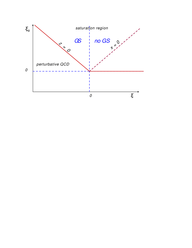
Figure 3: Saturation region: $z=\xi_{s}+\xi$ and $x=\xi_{s}-\xi$.

One can see that the general solution to Eq. (3.42) has the form:

$$\phi\left(\xi_{s},\xi\right)\,\,=\,\frac{1}{4}\xi_{s}\,\xi\,+\,F_{1}\left(\xi_{s}\right)\,+\,F_{2}\left(\xi\right)$$ (3.44)

and the solution of Eq. (3.42) can be obtained from Eq. (3.44) using the restriction from Eq. (2.35). For $t=z>x\;(\xi>0)$ we need to take into account the boundary condition of Eq. (3.41). Using the general solution in the form of Eq. (3.44) and the matching condition on the line $\xi=0$

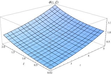
Fig. 4-a

Fig. 4-b

Figure 4: The exact solution of Eq. (2.31) for function $\phi\left(z,y\right)$(Fig. 4-a) and the dependence on $z$ at different values of $\xi$ (Fig. 4-b). $y=\xi_{s}$, $\xi_{s}=z-\xi$ and $\phi_{0}$ is taken to be equal to 0.1.

$$\phi_{1}\left(\xi=0\right)\,=\,\phi_{2}\left(\xi=0\right)$$ (3.45)

simultaneously with the boundary conditions that has the form

$$\phi_{2}\left(\xi_{s}=0\right)\,\,=\,\,\phi_{0}e^{\xi}$$ (3.46)

we obtain the following solution for $\xi>0$

$$\phi_{2}\left(z,\xi\right)\,\,=z^{2}/8\,-\,\xi^{2}/8\,+\,\phi_{0}\,e^{\xi}\,+\,\frac{1}{2}\phi_{0}\,\xi_{s}$$ (3.47)

Therefore, the solution to the simplified Eq. (3.42) has the following form

$$\phi\left(\right)\,\,=\,\,\left\{\begin{array}[]{l}\,\,\,\phi_{1}\left(z\right)\,\,\,\,\,\mbox{for}\,\,\,\xi\leq\,0\,;\\ \\ \,\,\,\phi_{2}\left(z,\xi\right)\,\,\,\,\,\mbox{for}\,\,\,\xi\,>\,0\,;\end{array}\right.$$ (3.51)

For the solution of the general Eq. (2.32) we have

$$\phi\left(\xi_{s},\,\xi;\,\right)\,\,=\,\,\left\{\begin{array}[]{l}\,\,\,\phi\left(z;\,{Eq.~{}(\ref{SOL})}\right)\,\,\,\,\,\mbox{for}\,\,\,\xi\leq\,0\,;\\ \\ \,\,z^{2}/8\,-\,\xi^{2}/8\,+\,\phi\left(\xi_{s};\,{Eq.~{}(\ref{SOL})}\right)\,-\,\phi_{0}\,+\,\phi_{0}\,e^{\xi}\,+\,\frac{1}{2}\phi_{0}\,\xi_{s}\,\,\,\,\,\mbox{for}\,\,\,\xi\,>\,0\,;\end{array}\right.$$ (3.55)

In Eq. (3.51) we assumed that for $\xi>0$ we are approaching the solution of Eq. (3.42).

One can see that solution of Eq. (3.55) does not show the geometric scaling behavior and solution of Eq. (2.32) depends both on $z$ and $\xi$. It happens so due to the influence of the boundary conditions.

In Fig. 4 we plot the numerical solution  of Eq. (2.32) in the region $\xi\,>\,0$ (see Fig. 4) with the following boundary conditions:

$$\phi\left(y\equiv\xi_{s},\xi=0\right)\,\, = \,\,\phi\left(\xi_{s}\right);$$

$$\phi\left(y\equiv\xi_{s}\,=\,0,\xi\right)\,\, = \,\,\phi_{0}\,e^{\xi};$$ (3.56)

One can see that this solution does not show the geometric scaling behavior inside the saturation domain.

To preserve the geometric scaling behavior we need to assume that for $\xi>0$ at $Y=Y_{0}$ the behavior of the scattering amplitude is not given by the Glauber
(McLerran-Venugopalan) formula but rather is determined by the solution of Eq. (2.36).

The initial condition based on McLerran-Venugopalan formula stems from the main assumption that there exists the rather low energy at which dipole rescatters in the nucleus but the emission of gluons can be neglected. At first sight, we do have arguments why the emission is small. Indeed, if $\bar{\alpha}_{S}^{2}A^{1/3}\approx 1$ for $\bar{\alpha}_{S}Y<1$ (or $Y\ll 1/\bar{\alpha}_{S}\approx 1/A^{1/6}$) the emission of the gluon will be suppressed while the Glauber-type rescattering will be essential since the interaction with the nucleus will be proportional to $\bar{\alpha}_{S}A^{1/3}\approx 1$. Therefore, we can choose the energy ($x$) which is large enough to use only the exchange of gluon for the dipole amplitude while the emission of gluon will be still suppressed. For this kinematic region we showed that the geometric scaling behavior of the amplitude is not valid. Since the McLerran-Venugopalan formula follows from the CGC approach and represents its key feature, we can claim that the CGC leads to the violation of the geometric scaling behavior in the kinematic region where $r^{2}\,Q_{s}\left(Y=Y_{0}\right)\,>\,1$.

However high density QCD has two facets at the moment: the color glass condensate CGC approach [4, 5, 6, 18] and the BFKL Pomeron calculus[9, 2, 3, 19, 20]. Both these approaches lead to the same non-linear Balitsky-Kovchegov equation [6, 7] for the dilute-dense system scattering in the large $N_{c}$ approximation which we consider here. However, in the BFKL Pomeron calculus the emission of gluons is taken into account even at small values of energy. In this approach the natural initial condition is $N^{eff}_{N}\left(r,Y=Y_{0}\right)\,\,=\,\,r^{2}\,Q_{s}(N;Y_{0})$ (compare with Eq. (3.40)) and the value of $Y_{0}$ is much smaller that $Y_{A}\,=\,(1/3)\ln A$. This case we consider in the next section.

Before doing this we would like to draw your attention to the fact that the condition $\bar{\alpha}_{S}^{2}A^{1/3}\approx 1$ can be reached in QCD only for scattering of states with typical extremely short distances (say, onium which made of two very heavy quarks). Running QCD coupling for such states could be small of the order of $\bar{\alpha}_{S}\sim 1/A^{1/6}$. For nuclei the typical $\bar{\alpha}_{S}$ is determined by the size of nucleons and could be as small as $\bar{\alpha}_{S}=0.2\div 0.3$ but not smaller. In this case the situation changes crucially: summing all powers of $\bar{\alpha}_{S}Y$ will lead us to the BFKL contribution namely $\bar{\alpha}_{S}^{2}e^{\omega_{0}Y}$. This contribution can be larger than the re-scattering in the classical gluon fields. It happens so at large $Y_{A}=\ln A^{1/3}$ since $\omega_{0}$ is larger that $1/3$ for $\bar{\alpha}_{S}=0.2\div 0.3$ (see Eq. (2.18)).

4 Solution for two critical lines

4.1 Equation for $Y<Y_{A}$

In the framework of the BFKL Pomeron calculus the rescattering with large rapidities but smaller than $Y_{A}=\ln A^{1/3}$ should be treated using the non linear equation. In this kinematic region each dipole interacts with the number of nucleons that are smaller than $\rho\,R_{A}\sim A^{1/3}$ and which actually is equal to $e^{Y}\rho/m$ where $\rho$ is the density of nucleons in the nucleus and $m$ is the proton mass[22, 23]. We can incorporate this observation into Eq. (2.1) by changing the definition of $T_{A}\left(b\right)$ in Eq. (2.4), namely,

$$T_{A}\left(b;Y\right)\,\,=\,\,\int^{+1/mx}_{-1/mx}dz\,\rho\left(b,z\right)$$ (4.1)

For $x\ll\,x_{A}=\,e^{-Y_{A}}$ Eq. (4.1) reduces to Eq. (2.4) while for $1\,\gg\,x\,\gg\,x_{A}$ Eq. (4.1) leads to $e^{Y}\rho/m$ for cylindrical nuclei.

Introducing

$$N_{A}\left(Y,\xi\right)\,\,=\,\,T_{A}\left(b;Y\right)\,N^{eff}_{N}\left(Y,\xi\right)$$ (4.2)

in stead of Eq. (2.29) and using $T_{A}\left(b;Y\right)$ in the form:

$$T_{A}\left(b;Y\right)\,\,=\,\,\left\{\begin{array}[]{l}\,\,\,\rho\,2R_{A}\,\propto\,A^{1/3}\,\,\,\,\,\mbox{for}\,\,\,Y\leq\,Y_{A}\,;\\ \\ \,\,\,e^{Y}\rho/m\,\,\,\,\,\mbox{for}\,\,Y\,<\,Y_{A}\,;\end{array}\right.$$ (4.6)

we can re-write Eq. (2.1) in the following form:

$$x\,<\,x_{A}\,\,(Y>Y_{A})\,\, : \frac{dN_{A}\Big{(}Y;\xi\Big{)}}{dY}\,\,=\,\,\bar{\alpha}_{S}\big{\{}\int^{\xi}_{\xi_{s}}\,d\xi^{\prime}N_{A}\Big{(}Y;\xi^{\prime}\Big{)}\,\,-\,\,N_{A}^{2}\Big{(}Y;\xi\Big{)}\Big{\}};$$ (4.7)

$$x\,>\,x_{A}\,\,(Y<Y_{A})\,\, : \frac{dN_{A}\Big{(}Y;\xi\Big{)}}{dY}\,-\,N_{A}\Big{(}Y;\xi\Big{)}\,\,=\,\,\bar{\alpha}_{S}\big{\{}\int^{\xi}_{\xi_{s}}\,d\xi^{\prime}N_{A}\Big{(}Y;\xi^{\prime}\Big{)}\,\,-\,\,N_{A}^{2}\Big{(}Y;\xi\Big{)}\Big{\}};$$ (4.8)

We will solve these two equations and these solutions should be matched on the line $Y=Y_{A}$ (see Fig. 1). These two equations have different critical lines. The critical line of the first one (see Eq. (4.7)) has been discussed in Eq. (2.19) and Eq. (2.20). It is shown as line 2 in Fig. 1 and has the form

$$\xi\,\,\equiv\,\,\ln\Big{(}r^{2}\,Q^{2}_{s}\left(A;Y_{A}\right)\Big{)}\,\,=\,\,-\,\xi_{2s}\,\,=\,\,-\,4\,\bar{\alpha}_{S}\,\left(Y\,-\,Y_{A}\right)$$ (4.9)

The easiest way to find the critical line for Eq. (4.8) is to search the solution to the general Eq. (2.1) with $T_{A}\left(b\right)$ replaced by $T_{A}\left(b;Y\right)$ in the semi-classical form

$$N_{A}\left(Y,\xi\right)\,\,=\,\,e^{S\left(Y,\xi\right)}\,\,=\,\,e^{\omega\left(Y,\xi\right)\,Y\,-\,\left(1-\gamma\left(Y;\xi\right)\right)\,\xi\,+\,S_{0}}$$ (4.10)

This solution has a form of wave-package and the critical line is the specific trajectory for this wave-package which coincides with the its front line. In other words, it is the trajectory on which the phase velocity ($v_{ph}$) for the wave-package is the same as the group velocity ( $v_{gr}$). The equation $v_{gr}\,\,=\,v_{ph}$ has the following form fort Eq. (4.8)

$$v_{ph}\,\,=\,\,\bar{\alpha}_{S}\frac{\chi\left(\gamma_{cr}\right)}{1\,-\,\gamma_{cr}}\,+\,\bar{\alpha}_{S}\frac{1}{1\,-\,\gamma_{cr}}\,\,=\,\,-\bar{\alpha}_{S}\chi^{\prime}\left(\gamma_{cr}\right)\,\,=\,\,v_{gr}$$ (4.11)

Solution to Eq. (4.11) gives $\gamma_{cr}\,\,=\,\,\sqrt{\bar{\alpha}_{S}}\,+\,{\cal O}(\bar{\alpha}_{S})$ and it leads to the equation (see Fig. 1)

$$\xi\,\,=\,\,-\xi_{1s}\,\,=\,\,\left(1\,+\,2\,\sqrt{\bar{\alpha}_{S}}\right)\left(Y_{A}-Y\right)$$ (4.12)

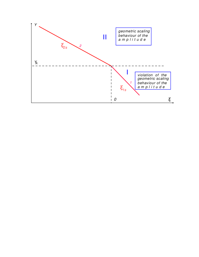
Figure 5: Two saturation regions for $N$: region I for $Y<Y_{A}=(1/3)\,\ln A$ and $\xi>\xi_{1s}=(1+2\sqrt{\bar{\alpha}_{S}})(Y_{A}-Y)$; and region II $Y>Y_{A}=(1/3),\ln A$ and $\xi\,>\,\xi_{2s}=-4\bar{\alpha}_{S}(Y-Y_{A})$. Here $\xi=\ln\left(r^{2}\,Q_{s}(Y=Y_{0};A)\right)$ where $r$ is the dipole size

4.2 Solutions

In both regions we will look for solutions using

$$\widetilde{N}_{A}\left(Y;\xi\right)\,\,=\,\,\int^{\xi}_{\xi_{is}}d\xi^{\prime}\,\Big{(}1\,-\,e^{-\phi\left(Y;\xi\right)}\Big{)}$$ (4.13)

In region II we obtain Eq. (2.31) which we need to solve with the same initial condition as in Eq. (2.35). As we have discussed Eq. (2.36) gives the solution of this problem.

In the region I using Eq. (4.13) we obtain after differentiation over $\xi$

$$\widetilde{N}_{A,Y\xi}\,-\,\widetilde{N}^{\prime}_{A,\xi}\,=\,\,\bar{\alpha}_{S}\widetilde{N}_{A}\left(1\,-\,\widetilde{N}^{\prime}_{A,\xi}\right)\;\;\mbox{or}\;\;\phi_{Y}\,e^{-\phi}\,-\,\left(1-e^{-\phi}\right)\,=\,\bar{\alpha}_{S}N_{A}e^{-\phi}$$ (4.14)

Differentiating Eq. (4.14) over $\xi$ we get

$$\phi_{Y\xi}-\phi_{Y}\,\phi_{\xi}-\phi_{\xi}\,=\,-\bar{\alpha}_{S}\widetilde{N}_{A}\phi_{\xi}+\bar{\alpha}_{S}\,\left(1-e^{-\phi}\right)$$ (4.15)

Eq. (4.15) has a simple solution for large $Y$ and $\xi$. Indeed, assuming that $\phi$ is large in this region , Eq. (4.15) can be re-written in the form

$$\phi_{Yz_{1}}\,-\,\phi_{z_{1}z_{1}}\,-\,\phi_{Y}\phi_{z_{1}}\,-\,\phi^{2}_{z_{1}}\,-\,\phi_{z_{1}}\,=\,-\bar{\alpha}_{S}z_{1}\phi_{z_{1}}\,+\,\bar{\alpha}_{S}\,$$ (4.16)

with $z_{1}\,=\,\,\xi+\xi_{1,s}\,=\,\left(1+2\sqrt{\bar{\alpha}_{S}}\right)\left(Y_{A}-Y\right)+\xi$.

One can see that the common solution of the two following equations

$$1.\,\,\,\,\phi_{Y\xi}\,\,=\,\,\bar{\alpha}_{S};\,\,\,\,\,\,\,\,\,2.\,\,\,\,\,\phi_{Y}+1\,=\,-\bar{\alpha}_{S}\,z_{1};$$ (4.17)

will be the solution of Eq. (4.16). It is easily seen that such a solution has the general form

$$\phi_{R1}\,\,=\,\ \bar{\alpha}_{S}\,\xi\,\left(Y_{A}-Y\right)\,+\,\bar{\alpha}_{S}(Y_{A}-Y)^{2}/2\,+\,\left(Y-Y_{A}\right)\,+\,F\left(\xi\right)$$ (4.18)

where $F\left(\xi\right)$ is the arbitrary function. The initial condition for this equation follows from the solution of Eq. (2.25) where $T_{A}\left(b\right)$ is replaced by $T_{A}\left(b;Y\right)$. They have the form

$$\phi_{R1}|_{\xi=\xi_{1s}}\,=\,\phi_{0}\,;\,\,\,\,\frac{d\phi_{R1}}{d\xi}|_{\xi=\xi_{1s}}\,=\,\phi_{0}$$ (4.19)

The boundary condition stems from the solution in region II (see Eq. (2.36)) and has the form

$$\phi_{R1}\left(Y=Y_{A};\xi\right)\,\,=\,\,\phi(\xi)$$ (4.20)

Choosing $F\left(\xi\right)=\phi\left(\xi\right)$ we see that solution $\phi_{R1}$ matchers the boundary condition of Eq. (4.20) but not the initial condition of Eq. (4.19). We need to solve Eq. (4.15) in the region of small $z_{1}$ to satisfy this condition, but in this region we cannot neglect the term $\exp\left(-\phi\right)$ in Eq. (4.15). We can approach this region solving Eq. (4.14) which can be rewritten in the form:

$$\phi_{Y}\left(Y,z_{1}\right)-e^{\phi\left(Y,z_{1}\right)}\,+\,1\,\,=\,\,\bar{\alpha}_{S}\widetilde{N}_{A}\left(Y;z_{1}\right)$$ (4.21)

with

$$\widetilde{N}_{A}\left(Y;z_{1}\right)\,\,=\,\,\int^{z_{1}}_{0}dz^{\prime}_{1}\,\Big{(}1\,-\,e^{-\phi\left(Y;z^{\prime}_{1}\right)}\Big{)}$$ (4.22)

After differentiation of Eq. (4.21) with respect to $z_{1}$ one obtains

$$\phi_{Y,z_{1}}\left(Y,z_{1}\right)\,-\,\phi_{z_{1}}\left(Y,z_{1}\right)\,e^{\phi\left(Y,z_{1}\right)}\,\,=\,\,\bar{\alpha}_{S}\Big{(}1\,-\,e^{-\phi\left(Y,z_{1}\right)}\Big{)}$$ (4.23)

The initial and boundary conditions for Eq. (4.23) looks as follows:

initial conditions: $$\phi\left(Y,z_{1}=0\right)\,=\,\phi_{0}\,;$$

boundary conditions: $$\phi\left(Y=0,z_{1}\right)\,=\,\phi\left(z^{\prime}_{1}\right)\,;$$ (4.24)

This equation has been solved numerically and the solution for $\phi$ and $N_{A}=1-\exp\Big{(}-\phi\Big{)}$ is shown in Fig. 6.

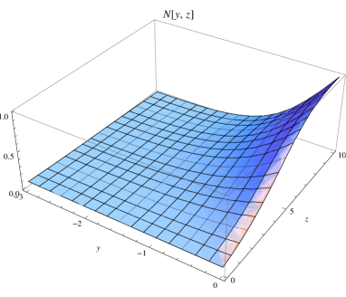
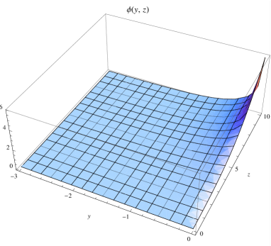
Fig. 6-a	Fig. 6-b

Figure 6: The exact solution of Eq. (4.23) for function $N_{A}\left(y,z\right)\,\equiv\,N\left(y,z\right)$ (Fig. 6-a) and $\phi$ (Fig. 6-b). $y=\xi_{1s}$, $\xi_{1s}=z_{1}-\xi$ and $\phi_{0}$ is taken to be equal to 0.1 and $\bar{\alpha}_{S}=0.2$.

Therefore, the full solution has the geometric scaling behavior in the region II but shows the violation of the scaling behavior in region I as it follows from Eq. (4.18) and Fig. 6.

Comparing this result with the conclusions of the previous section we see that the BFKL Pomeron calculus predicts the geometric scaling behavior in the saturation region for $r^{2}\,Q^{2}_{s}\left(A;Y_{0}\right)\,>\,1$ and $Y>Y_{A}$.

5 Impact parameter dependence of the scattering amplitude

In this section we complete the study of the impact parameter dependence of the scattering amplitude that has been started in Ref.[24]. In Ref.[24] we claim that in the framework of the BK equation with the simplified kernel the impact parameter dependence can be absorbed into redefinition of the saturation scale, namely,

$$\mbox{For proton}\,\,\,\tau\,\equiv\,r^{2}\,Q^{2}_{s}(P;x)\,\,\,\longrightarrow\,\,\,\,r^{2}\,Q_{s}(A;x)\;\;\mbox{with}\;\;Q_{s}\left(A;x\right)\,=\,T^{2}_{A}\left(b\right)\,Q^{2}_{s}\left(P;x\right)\,\,\equiv\,\,\tau_{A}\,\,\,\,\mbox{for nuclei}$$ (5.25)

or

$$z_{\mbox{proton}}\,\,\,\longrightarrow\,\,\,\,z_{\mbox{nucleus}}\,\,=\,\,z_{\mbox{proton}}\,\,\,+\,\,\,2\,\ln\Big{(}T_{A}\left(b\right)\Big{)}$$ (5.26)

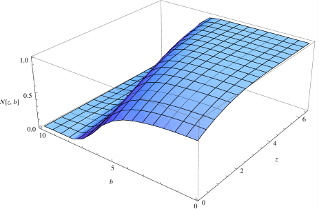
Fig. 7-a	Fig. 7-b

Figure 7: The exact solution of Eq. (2.37) for function $N\left(z,b\right)=1-\exp\left(-\phi\left(z,b\right)\right)$ (Fig. 7-a) for the interaction of the dipole with the gold and its dependence on $b$ at different values of $z$ (Fig. 7-b). $y=\xi_{s}$, $\xi_{s}=z-\xi$ and $\phi_{0}$ is taken to be equal to 0.1.

However, this claim is based on the solution of Eq. (2.36) which assumed that $\phi_{0}\,\ll\,1$. In the general solution of Eq. (2.37) one can see that $b$-dependence cannot be reduced to changes in the value of the saturation scale. In Fig. 7 we plot the dependence of the scattering amplitude on the impact parameter using the realistic $T_{A}\left(b\right)$ for the gold[25] and the value of $\phi_{0}$ in Eq. (2.25) taken from the fit of the HERA data [26]. The first glance at Fig. 7 shows that the typical value of $b$ increases with $z$. It has a natural explanation. Indeed the width $b_{o}$ of $b$ distribution we can define as $N\left(z,b=b_{0}\right)=e^{-1}$. Since the amplitude $N$ has the geometric scaling behavior the value of $b_{0}$ can be determined from the equation

$$N_{A}\left(\tau_{A}\right)\,\,=\,\,N_{A}\Big{(}T^{2}_{A}\left(b_{0}\right)\,Q^{2}_{s}\left(P;x\right)\Big{)}\,\,=\,\,e^{-1}\,\,$$ (5.27)

where $Q_{s}\left(P;x\right)$ is the saturation scale for the proton target. In other words, the typical $b$ can be determined from the following equation:

$$T^{2}_{A}\left(b_{0}\right)\,Q^{2}_{s}\left(P;x\right)\,\,\,=\,\,\tau_{A}\,\,=\,\,\,\mbox{Const}$$ (5.28)

Recalling that

$$Q^{2}_{s}\left(P;x\right)\,\,=\,\,Q^{2}_{0}\Big{(}\frac{1}{x}\Big{)}^{\lambda}\,\,\,\,\,\,\mbox{with}\,\,\,\,\,\,\,\,\lambda\,=\,4\bar{\alpha}_{S}$$ (5.29)

one can see that

$$b_{0}\,=\,\,R_{A}\,\,+\,\,\frac{1}{2}\,h\,\lambda\ln(1/x)$$ (5.30)

where we use that

$$T_{A}\left(b_{0}\right)\,\,\,\,\,\,\xrightarrow{b>R_{A}}\,\,\,\,\,\,e^{-\frac{b-R_{A}}{h}}$$ (5.31)

and $h$ is about $0.5\,fm$.

In terms of $z$ Eq. (5.31) has even a simpler form:

$$b\,\,=\,\,R_{A}\,+\frac{h}{2}\,z_{\mbox{proton}}$$ (5.32)

It is wort mentioning that Eq. (5.32) does not depend on the specific form of energy dependence of the saturation momentum.

It should be stressed that we obtain a logarithmic increase of the radius of interaction with $z$. It stems from Eq. (2.1) where we have integrated over the impact parameter of the nucleon. As we have discuss we can trust this $b$-dependence in the kinematic region of Eq. (2.7). Certainly, for the dipole-gold scattering for $z\leq 7$ we can use this Glauber-type approximation. All problems with $b$-dependence are originated from the large $b$ dependence of the dipole-proton amplitude which falls down as $1/b^{4}$ in perturbative QCD[12]. Implicitly we assumed that the non-perturbative corrections to the B-K equation has been taken into account for dipole-nucleon scattering in the transition from Eq. (2) to Eq. (2.1).

Figure 8: Total cross section for dipole-gold amplitude $\sigma_{tot}=2\int d^{2}b\,N\left(z,b\right)$ in the saturation region: the solution of Eq. (2.37) (curve 1) and the solution to Eq. (2.32) with simplified $T_{A}\left(b\right)\,\varpropto\,\Theta\left(R_{A}-b\right)$ (curve 2).

In Fig. 8 we plotted the dependence on $z$ the total cross section of dipole-nucleus intertaction for the case of gold

$$\sigma_{tot}\,\,=\,\,2\int d^{2}b\,N\left(z,b\right)$$ (5.33)

One can see a significant difference between realistic Wood-Saxon $T_{A}\left(b\right)$ and the simplified one $T_{A}\left(b\right)\,=\,\rho\,\Theta\left(R_{A}-b\right)$ where $\rho$ is the density of the nucleons in the nucleus. This picture demonstrates the significance of correct $b$-dependence for calculation of the physical observables.

6 Conclusions

We hope that we answered three questions that we have discussed in the introduction. The first one: could the initial conditions affect the behavior of the scattering amplitude at $\tau\,\gg\,1$. The answer is yes and we gave the explicit solution of Balitsky-Kovchegov equation which shows the violation of the geometric scaling behavior of the scattering amplitude if you use the McLerran  -  Venugopalan formula as the initial condition .

The second question: can we trust the McLerran-Venugopalan formula deeply in the saturation region, has a kind of negative answer. In the sense that the McLerran-Venugopalan formula cannot be considered as the unique initial condition. We demonstrated that in the BFKL Pomeron calculus this formula should be replaced by the solution to the non linear equation in the region of $Y<Y_{A}=\ln(A^{1/3})$ for very heavy nuclei. This statement gives the answer to the third question: what initial condition we need to use to reproduce the geometric scaling behavior.

It is well known that we have two approaches to high density QCD; the BFKL Pomeron calculus[2, 3, 19, 20] and Color Glass Condensate[4, 5, 6, 7]. Both lead to the same Balitsky-Kovchegov equation for DIS. The difference between them lays in the initial conditions. For the CGC the initial condition is the McLerran-Venugopalan formula which is valid in the classical gluon field approximation. On the other hand, for the BFKL Pomeron calculus a natural initial condition stems from the solution of B-K equation for $Y<Y_{A}$. Therefore, we can formulate the main result of the paper in the following way. The CGC approach leads to the violation of the geometric scaling behavior for DIS with heavy nuclei for $r^{2}\,Q_{s}\left(A;Y=Y_{0}\right)\,>\,1$ while the BFKL Pomeron calculus leads to the geometrical scaling behavior of the amplitude for $Y>Y_{A}$. This result gives a possibility to check experimentally which of these two approaches is more adequate.

References

- [1] J. Bartels, E. Levin, Nucl. Phys. B387 (1992) 617-637.
- [2] L. V. Gribov, E. M. Levin and M. G. Ryskin, Phys. Rep. 100, 1 (1983).
- [3] A. H. Mueller and J. Qiu, Nucl. Phys.,427 B 268 (1986) .
- [4] L. McLerran and R. Venugopalan, Phys. Rev. D 49,2233, 3352 (1994); D 50,2225 (1994); D 53,458 (1996); D 59,09400 (1999).
- [5] J. Jalilian-Marian, A. Kovner, A. Leonidov and H. Weigert, Phys. Rev. D59, 014014 (1999), [arXiv:hep-ph/9706377]; Nucl. Phys. B504, 415 (1997), [arXiv:hep-ph/9701284]; J. Jalilian-Marian, A. Kovner and H. Weigert, Phys. Rev. D59, 014015 (1999), [arXiv:hep-ph/9709432]; A. Kovner, J. G. Milhano and H. Weigert, Phys. Rev. D62, 114005 (2000), [arXiv:hep-ph/0004014] ; E. Iancu, A. Leonidov and L. D. McLerran, Phys. Lett. B510, 133 (2001); [arXiv:hep-ph/0102009]; Nucl. Phys. A692, 583 (2001), [arXiv:hep-ph/0011241]; E. Ferreiro, E. Iancu, A. Leonidov and L. McLerran, Nucl. Phys. A703, 489 (2002), [arXiv:hep-ph/0109115]; H. Weigert, Nucl. Phys. A703, 823 (2002), [arXiv:hep-ph/0004044].
- [6] I. Balitsky, [arXiv:hep-ph/9509348]; Phys. Rev. D60, 014020 (1999) [arXiv:hep-ph/9812311]
- [7] Y. V. Kovchegov, Phys. Rev. D60, 034008 (1999), [arXiv:hep-ph/9901281].
- [8] E. Iancu, K. Itakura, L. McLerran, Nucl. Phys. A708 (2002) 327-352. [hep-ph/0203137]
- [9] E. A. Kuraev, L. N. Lipatov, and F. S. Fadin, Sov. Phys. JETP 45, 199 (1977); Ya. Ya. Balitsky and L. N. Lipatov, Sov. J. Nucl. Phys. 28, 22 (1978).
- [10] E. Levin, K. Tuchin, Nucl. Phys. A693 (2001) 787-798. [hep-ph/0101275].
- [11] A. M. Stasto, K. J. Golec-Biernat, J. Kwiecinski, Phys. Rev. Lett. 86 (2001) 596-599, [hep-ph/0007192]; L. McLerran, M. Praszalowicz, Acta Phys. Polon. B42 (2011) 99, [arXiv:1011.3403 [hep-ph]] B41 (2010) 1917-1926, [arXiv:1006.4293 [hep-ph]]. M. Praszalowicz, [arXiv:1104.1777 [hep-ph]], [arXiv:1101.0585 [hep-ph]].
- [12] A. Kovner and U. A. Wiedemann, Phys. Lett. B 551 (2003) 311 [arXiv:hep-ph/0207335]; Phys. Rev. D 66 (2002) 034031 [arXiv:hep-ph/0204277]; Phys. Rev. D 66 (2002) 051502 [arXiv:hep-ph/0112140].
- [13] E. Levin and K. Tuchin, Nucl. Phys. A691 (2001) 779,[arXiv:hep-ph/0012167]; B573 (2000) 833, [arXiv:hep-ph/9908317].
-
[14]
V. N. Gribov and L. N. Lipatov, Sov. J. Nucl. Phys 15 (1972)
438;
G. Altarelli and G. Parisi, Nucl. Phys. B 126 (1977) 298;
Yu. l. Dokshitser, Sov. Phys. JETP 46 (1977) 641. - [15] S. Munier and R. B. Peschanski, Phys. Rev. D 70 (2004) 077503 [arXiv:hep-ph/0401215]; Phys. Rev. D 69 (2004) 034008 [arXiv:hep-ph/0310357]; Phys. Rev. Lett. 91 (2003) 232001 [arXiv:hep-ph/0309177].
- [16] A. H. Mueller and D. N. Triantafyllopoulos, Nucl. Phys. B640 (2002) 331 [arXiv:hep-ph/0205167]; D. N. Triantafyllopoulos, Nucl. Phys. B648 (2003) 293 [arXiv:hep-ph/0209121].
- [17] Andrei D. Polyanin and Valentin F. Zaitsev, “ Handbook of nonlinear Partial Differential Equations”, Chapman Hall/CRC, 2004.
- [18] T. Altinoluk, A. Kovner and M. Lublinsky, JHEP 0903 (2009) 110 [arXiv:0901.2560 [hep-ph]]; JHEP 0903 (2009) 109 [arXiv:0901.2559 [hep-ph]; A. Kovner and M. Lublinsky, JHEP 0611 (2006) 083 [arXiv:hep-ph/0609227]; Nucl. Phys. A 767 (2006) 171 [arXiv:hep-ph/0510047]; Phys. Rev. D 72 (2005) 074023 [arXiv:hep-ph/0503155]; Phys. Rev. Lett. 94 (2005) 181603 [arXiv:hep-ph/0502119]; JHEP 0503 (2005) 001 [arXiv:hep-ph/0502071];
- [19] M. A. Braun, Phys. Lett. B632 (2006) 297 [arXiv:hep-ph/0512057]; arXiv:hep-ph/0504002 ; Eur. Phys. J. C16, 337 (2000) [arXiv:hep-ph/0001268]; Phys. Lett. B 483 (2000) 115 [arXiv:hep-ph/0003004]; Eur. Phys. J. C 33 (2004) 113 [arXiv:hep-ph/0309293]; Eur. Phys. J. C6, 321 (1999) [arXiv:hep-ph/9706373]; M. A. Braun and G. P. Vacca, Eur. Phys. J. C6, 147 (1999) [arXiv:hep-ph/9711486].
- [20] J. Bartels, M. Braun and G. P. Vacca, Eur. Phys. J. C40, 419 (2005) [arXiv:hep-ph/0412218] ; J. Bartels and C. Ewerz, JHEP 9909, 026 (1999) [arXiv:hep-ph/9908454] ; J. Bartels and M. Wusthoff, Z. Phys. C66, 157 (1995) ; A. H. Mueller and B. Patel, Nucl. Phys. B425, 471 (1994) [arXiv:hep-ph/9403256]; J. Bartels, Z. Phys. C60, 471 (1993).
- [21] E. Levin, J. Miller and A. Prygarin, Nucl. Phys. A 806 (2008) 245 [arXiv:0706.2944 [hep-ph]].
- [22] E. Levin and M. G. Ryskin,, Sov. J. Nucl. Phys. 41, (1985), 300 [Yad. Fiz. 41, (1985) 472].
- [23] J. w. Qiu, Nucl. Phys. B 291,( 1987) 74.
- [24] A. Kormilitzin, E. Levin, Nucl. Phys. A849 (2011) 98-119. [arXiv:1009.1468 [hep-ph]].
- [25] C. W. De Jager, H. De Vries, C. De Vries, Atom. Data Nucl. Data Tabl. 14 (1974) 479-508.
- [26] G. Watt, H. Kowalski, Phys. Rev. D78, 014016 (2008), [arXiv:0712.2670 [hep-ph]]; H. Kowalski, L. Motyka, G. Watt, Phys. Rev. D74 (2006) 074016, [hep-ph/0606272].