Spectral action, Weyl anomaly and the Higgs-Dilaton potential

Abstract:

We show how the bosonic spectral action emerges from the fermionic action by the renormalization group flow in the presence of a dilaton and the Weyl anomaly. The induced action comes out to be basically the Chamseddine-Connes spectral action introduced in the context of noncommutative geometry. The entire spectral action describes gauge and Higgs fields coupled with gravity. We then consider the effective potential and show, that it has the desired features of a broken and an unbroken phase, with the roll down.

1 Introduction

In this note we will show the intimate relationships between Weyl anomalies, the dilaton and the Higgs field in the framework of spectral physics. The framework is the expression of a field theory in terms of the spectral properties of a (generalized) Dirac operator. In this respect this work can be seen in the framework of the noncommutative geometry approach to the standard model of Connes and collaborators [1, 2, 3, 4], as well as of Sakharov induced gravity [5] (for a modern review see [6]).

We start with a generic action for a chiral theory of fermions coupled to gauge fields and gravity. The considerations here apply to the standard model, but we will not need the details of the particular theory under consideration. It is known, and this is the essence of the noncommutative geometry approach to the standard model, that the theory is described by a fermionic action and a bosonic action, both of which can be expressed in terms of the spectrum of the Dirac operator. In [7] two of us have shown that if one starts from the classic fermionic action and proceeds to quantize the theory with a regularization based on the spectrum, an anomaly appears. it is possible that the full quantum theory is still invariant by correcting the path integral measure. This is tantamount to the addition of a term to the action, which renders the bosonic background interacting to the dilaton field. The main result of that paper is that this term is a modification of the bosonic spectral action [3]. In this case the theory is still invariant.

In this paper we have a shift of the point of view. We still consider the theory to be regularized in the presence of a cutoff scale, but we consider this scale to have a physical meaning, that of the breaking of Weyl invariance. We then consider the flow of the theory at a renormalization scale, which is not necessarily the scale which breaks the invariance. The theory has a dilaton, and the Higgs field.

The dilaton may involve a collective scalar mode of all fermions accumulated in a Weyl-noninvariant dilaton action. Accordingly the spectral action arises as a part of the fermion effective action divided into the Weyl non-invariant and Weyl invariant parts.

We calculate the dilaton effective potential and we discuss how it relates to the transition from the radiation phase with zero vacuum expectation value of Higgs fields and massless particles to the electroweak broken phase via condensation of Higgs fields. The collective field of dilaton can provide the above mentioned phase transition with EW symmetry breaking during the evolution of the universe.

The next five Sections of the paper will present the general framework, namely the Weyl invariance of fermions in a fixed background described via the (generalized) Dirac operator in Section 2, the connections with noncommutative geometry, the Weyl invariance properties, the spectral action and the bosonic action in the the following Sections. These sections mostly follow reference [7], although the point of view presented in Sect. 5 is different, and in particular show two possible ways to obtain the spectral action, which is briefly introduced in Sect. 6. The cosmological implications are discussed in Sec. 7. This material has not been previously published, but parts of it have been presented in a conference [8]. A final Section contains the conclusions.

2 Fermions in a Fixed Background

Our starting point is a theory in which we have some matter fields, represented by fermions transforming under some (reducible) representation a gauge group, such as the standard model group $SU(3)\times SU(2)\times U(1)$. We need not specify the group for the moment. The fermions will be spinors belonging to some Hilbert space $\cal H$ which we assume to be “chiral”, i.e. split into a left and a right spaces:

$${\cal H}={\cal H}_{L}\oplus{\cal H}_{R}$$ (1)

A generic matter field will therefore be a spinor

$$\Psi=\begin{pmatrix}\Psi_{L}\\ \Psi_{R}\end{pmatrix}$$ (2)

and in this representation the chirality operator, which we call $\gamma$, is a two by two diagonal matrix with plus and minus one eigenvalues. The two components are spinors themselves and we are not indicating the gauge indices, nor the flavor indices. We will assume that the fermions come in a number of identical generations, distinguished only by the masses (or more precisely their Yukawa coupling).

The dynamics of the fermions is given by coupling them to a gauge and gravitational background. This coupling is performed by a classical action, which we schematically write as:

$$S_{F}=\left\langle\Psi\right|D\left|\Psi\right\rangle$$ (3)

The operator $D$ [3] is a $2\times 2$ matrix acting on spinors of the kind (2)

$$D=\left(\begin{array}[]{cc}i\gamma^{\mu}D_{\mu}+{\mathbb{A}}&\gamma_{5}S\\ \gamma_{5}S^{\dagger}&i\gamma^{\mu}D_{\mu}+{\mathbb{A}}\end{array}\right)$$ (4)

where

$$D_{\mu}=\partial_{\mu}+\omega_{\mu},$$ (5)

the quantity $\omega_{\mu}$ is the spin connection, $\mathbb{A}$ contains all gauge fields of the theory and $S$ contains the information about Higgs field, Yukawa couplings, mixings and all terms which couple the left and right part of the spinors. The gravitational background is in general nontrivial, and the metric is encoded in the anticommutator of the $\gamma$’s: $\{\gamma^{\mu},\gamma^{\nu}\}=2g^{\mu\nu}$.

The quantity $\mathbb{A}$ represents instead a fixed gauge background, and the interaction of the spinors with it. We emphasize that at this stage we are just describing the classical dynamics of fermions in a fixed background. We are deliberately vague as to the detail of the model at this stage, not discussing important elements of the theory, like chirality or charge conjugation. The scheme presented here is largely independent on the details of the model. In particular it applies to the standard model, especially in the approach based on noncommutative geometry introduced by Connes, which we briefly describe in Sect. 5.

3 Weyl invariance and the Fermionic Action

The fermionic action (3) in invariant under the transformation

$$\left|\Psi\right\rangle \to {\rm e}^{\frac{\phi}{2}}\left|\Psi\right\rangle$$

$$D \to {\rm e}^{-\frac{\phi}{2}}D{\rm e}^{-\frac{\phi}{2}}$$ (6)

where the operator $\phi$ is a function of the (operator) $x$, or in a simpler case a constant. The action (3) can be expressed in coordinates as

$$S_{F}=\int d^{4}x\sqrt{|g|}\psi(x)^{\dagger}D_{x}\psi(x);\quad(|g|)^{1/4}\psi(x)=\langle{x}\left|\Psi\right\rangle$$ (7)

where we introduced the subscript $x$ on $D$ to stress the fact that it is an operator acting on the $x$ coordinate. The transformation (6) can be seen as a (generalized) Weyl transformation:

$$g_{\mu\nu}(x) \to {\rm e}^{2\phi(x)}g_{\mu\nu}(x)$$

$$\psi(x) \to {\rm e}^{-\frac{3}{2}\phi(x)}\psi(x)$$

$$(D_{x}\psi(x)) \to {\rm e}^{-\frac{5}{2}\phi(x)}(D_{x}\psi(x))$$ (8)

where $\phi(x)$ is real. Note that since the rescaling involves also the matrix part of $D$, we must also rescale the masses of the fermions. In this sense we differ form the usual usage of Weyl (or conformal) invariance which is only valid for massless fields. In our scheme Yukawa couplings are an integral part of the Dirac operator which encodes all metric properties of the “noncommutative manifold” described by the noncommutative matrix algebra. In the absence of a dimensional scale, this is an exact symmetry of the classical theory.

We now proceed to quantize the theory. It can be proven [9] that if the classical theory is invariant, the measure in the quantum path integral is not. We have an anomaly: a classical theory is invariant against a symmetry transformation, but the quantum theory, due to unavoidable regularization, does not possess this symmetry anymore. If also the quantum theory is required to be symmetric then the symmetry can be restored by the addition of extra terms in the action, alternatively one should have a fundamental length in the theory to explain violation of Weyl invariance. A textbook introduction to anomalies can be found in [9]. The notion of Weyl anomaly is attached to the dilatation of both coordinates, fields and mass-like parameters according to their dimensionalities, Eq. (8). Evidently, in the absence of UV divergences, there is no Weyl anomaly which therefore can be correlated to rescaling of a cutoff in the theory. In the case when the dilatation is not constant, $\phi$ becomes a quantum field called the dilaton. The dilaton of this kind has been investigated in the context of the spectral action in [10].

We remark that there may be also an alternative realization of the dilaton as a collective scalar mode of all fermions accumulated in a scale-noninvariant dilaton action (in the spirit of [11]).

We start from the partition function

$$Z(D,\mu)=\int[{\rm d}\psi][{\rm d}\bar{\psi}]e^{-S_{\psi}}=\det\left(\frac{D}{\mu}\right)$$ (9)

where we needed to introduce a normalization scale $\mu$ for dimensional reasons, and the last equality is formal because the expression is divergent and needs regularizing. The writing of the fermionic action in this form (as a Pfaffian) is instrumental in the solution of the fermion doubling problem in Connes approach to the standard model [12, 13, 4].

In order to regularize the expression (9) we need to introduce a cutoff scale, which we call $\Lambda$. This is the cutoff scale and it may have the physical meaning of an energy in which the theory (seen as effective) has a phase transition, or at any rate a point in which the symmetries of the theory are fundamentally different (unification scale).

We then have two scales, and we will keep them separated although in principle, at this stage, they could be identified. We will see in the course of this work that they cannot actually be identical, although have to be of the same order of magnitude.

We will regularize the theory in the ultraviolet using a procedure introduced by one of us, Bonora and Gamboa-Saravi in [16, 17, 18] but leaving room for the normalization scale $\mu$. Although this procedure predates the spectral action, it is very much in the spirit of spectral geometry, since it uses only the spectral data of the Dirac operator. The energy cutoff is enforced by considering only the first $N$ eigenvalues of $D$. Consider the projector

$$P_{N}=\sum_{n=1}^{N}\left|\lambda_{n}\right\rangle\left\langle\lambda_{n}\right|;\quad N=\max n\ \mbox{such that}\ \lambda_{n}\leq\Lambda$$ (10)

where $\lambda_{n}$ are the eigenvalues of $D$ arranged in increasing order of their absolute value (repeated according to possible multiplicities), $\left|\lambda_{n}\right\rangle$ a corresponding orthonormal basis, and the integer $N$ is a function of the cutoff. This means that we are effectively using the $N^{\mathrm{th}}$ eigenvalue as cutoff. Therefore this number and the corresponding spectral density depends on coefficient functions of the Dirac operator, $N=N(D)$.

Instead of this sharp cutoff, which consider totally all eigenvalues up to a certain energy, and ignore all the rest of the spectrum, it is also possible to consider a smooth cutoff enforced by a smooth function. Choosing a function $\chi$ which is smoothened version of the characteristic function of the interval $[0,1]$ one can consider the operator

$$P_{\chi}=\chi\left(\frac{D}{\Lambda}\right)=\sum_{n}\chi\left(\frac{\lambda_{n}}{\Lambda}\right)\ \left|\lambda_{n}\right\rangle\left\langle\lambda_{n}\right|.$$ (11)

This operator is not a projector anymore, and it coincides with $P_{N}$ for $\chi=\Theta$, where $\Theta$ is the Heaviside step function.. The use of a smooth $\chi$ can be preferable in an expansion, such as the heat kernel expansion we will perform later in Sect.5.2 for the spectral action. Nevertheless for the scopes of the present paper a sharp cutoff is adequate.

In the framework of noncommutative geometry this is the most natural cutoff procedure, although as we said it was introduced before the introduction of the standard model in noncommutative geometry. It makes no reference in principle to the underlying structure of spacetime, and it is based purely on spectral data, thus is perfectly adequate to Connes’ programme. This form of regularization could be also used for field theory which cannot be described on an ordinary spacetime, as long as there is a Dirac operator, or generically a wave operator, with a discrete spectrum.

We define the regularized partition function

$$Z(D,\mu) = \prod_{n=1}^{N}\frac{\lambda_{n}}{\mu}=\det\left(\mbox{1 \kern-5.30997pt{\rm l}}-P_{N}+P_{N}\frac{D}{\mu}P_{N}\right)$$ (12)

$$= \det\left(\mbox{1 \kern-5.30997pt{\rm l}}-P_{N}+P_{N}\frac{D}{\Lambda}P_{N}\right)\det\left(\mbox{1 \kern-5.30997pt{\rm l}}-P_{N}+\frac{\Lambda}{\mu}P_{N}\right)$$

$$= Z_{\Lambda}(D,\Lambda)\det\left(\mbox{1 \kern-5.30997pt{\rm l}}-P_{N}+\frac{\Lambda}{\mu}P_{N}\right).$$

In this way we can define the fermionic action in an intrinsic way.

The regularized partition function $Z(D,\Lambda)$ has a well defined meaning. Expressing $\psi$ and $\bar{\psi}$ as

$$\psi=\sum_{n=1}^{\infty}a_{n}\left|\lambda_{n}\right\rangle;\qquad\bar{\psi}=\sum_{n=1}^{\infty}b_{n}\left|\lambda_{n}\right\rangle$$ (13)

with $a_{n}$ and $b_{n}$ anticommuting (Grassman) quantities. Then $Z(D,\Lambda)$ becomes (performing the integration over Grassman variables for the last step)

$$Z(D,\Lambda)=\int\prod_{n=1}^{N}\dfrac{{\rm d}a_{n}{\rm d}b_{n}}{\Lambda}{\rm e}^{-\sum_{n=1}^{N}b_{n}\lambda_{n}a_{n}}=\det\left(D_{N}\right)$$ (14)

where we defined

$$D_{N}=1-P_{N}+P_{N}\frac{D}{\Lambda}P_{N}.$$ (15)

In the basis in which $D/\Lambda$ is diagonal it corresponds to set to $\Lambda$ all eigenvalues of $D$ larger than $\Lambda$. Note that $D_{N}$ is dimensionless and depends on $\Lambda$ both explicitly and intrinsically via the dependence of $N$ and $P_{N}$.

It is possible to give an explicit functional expression to the projector in terms of the cutoff:

$$P_{N}=\Theta\left(1-\frac{D^{2}}{\Lambda^{2}}\right)=\int\limits_{-\infty}^{\infty}{\rm d}\alpha\,\frac{1}{2\pi{\rm i}(\alpha-{\rm i}\epsilon)}{\rm e}^{{\rm i}\alpha\big{(}1-\frac{D^{2}}{\Lambda^{2}}\big{)}}$$ (16)

This integral is well defined for a compactified space volume. Actually $N$ depends also on the infrared cutoff, and the number of dimensions.

4 Bosonic Action from Weyl Anomaly

In this section we will see how the Weyl anomaly induces the bosonic part of the action. The induced action is the Chamseddine-Connes spectral action.

The action $S_{\psi}$ is invariant under (8), but the partition function (9) is not. The reason for this is the fact that the regularization procedure is not Weyl invariant. In [7] it was shown that the anomaly can in principle be absorbed by a change of the measure, which is equivalent to the addition of another term to the action. This term can compensate the change in the measure due to the regularization, but being in an exponential form, can also be seen as another addition to the action, so that the final partition function is invariant. This calculation has been originally performed in [19] in the QCD context, and applied to gravity in [20]. In the scenario we are favoring in this paper however Weyl symmetry is not an exact symmetry of the theory, and the bosonic part of the action is induced by the renormalization group flow.

In the following we will mostly consider the case of $\phi$ constant (i.e. not depending on $x$). This simplifies things because we do not have to worry about the kinetic terms of the field, and renders the functional integrals simple integrals.

In order to make contact with the spectral action (to be discussed next) let us notice that $N$ is just the number of eigenvalues smaller that $\Lambda$, and thereby

$$\>{\rm Tr}\,\chi\left(\frac{D^{2}}{\Lambda^{2}}\right)=\>{\rm Tr}\,\Theta\left(1-\frac{D^{2}}{\Lambda^{2}}\right)=\>{\rm Tr}\,P_{N}=N(\Lambda,\ D).$$ (17)

where $\chi$ is a generic cutoff function, which in our case is a sharp cutoff at energy $\Lambda$,

$$\chi(x)=\left\{\begin{array}[]{cc}0{}&x<0\\ 1{}&x\in[0,1]\\ 0{}&x>1\end{array}\right.$$ (18)

consequence of the sharp cutoff on the eigenvalues used in (10). For smoother cutoffs of the eigenvalues this would reflect in different forms of $\chi$. We will see in the next section that at one loop level (the only doable approximation) the actual form of the cutoff is not crucial. The latter form or (17) is valid provided that we take into account the functional dependence $N=N(\Lambda,\ D)$. It is worth recalling again that the integer $N$ depends on the cutoff $\Lambda$, on the Dirac operator $D$ and also on the function $\chi$ which we have chosen to be a sharp cutoff.

If we want to obtain a partition function invariant on $\phi$ we can integrate it out, i.e.

$$Z_{\mathrm{inv}}(D,\mu)=\int{\rm d}\phi Z({\rm e}^{-\frac{1}{2}\phi}D{\rm e}^{-\frac{1}{2}\phi},\mu)\equiv\int{\rm d}\phi Z(D_{\phi},\mu);\qquad D_{\phi}\equiv{\rm e}^{-\frac{1}{2}\phi}D{\rm e}^{-\frac{1}{2}\phi}.$$ (19)

This was the procedure followed in [7]. Notice however that in principle we could have equally well defined

$$\hat{Z}_{\mathrm{inv}}(D,\mu)=\left(\int{\rm d}\phi\dfrac{1}{Z(D_{\phi},\mu)}\right)^{-1}.$$ (20)

If we consider non Weyl invariant partition function we can split it in the product of a term invariant for Weyl transformations, and another not invariant, which will depend on the field $\phi$.

$$Z(D,\mu)=\hat{Z}_{\mathrm{inv}}(D,\mu)Z_{\mathrm{not}}(D,\mu)$$ (21)

The terms in $Z_{\mathrm{not}}$ are due to the Weyl anomaly and we can calculate them. Using

$$D_{\phi}={\rm e}^{-\frac{1}{2}\phi}D{\rm e}^{-\frac{1}{2}\phi}$$ (22)

consider the identity

$$Z(D)=\left(\int[d\phi]\frac{1}{Z(D_{\phi})}\right)^{-1}\,\int[d\phi]\frac{Z(D)}{Z(D_{\phi})}$$ (23)

Since the first term is invariant by construction, the second is the not invariant one:

$$Z_{\mathrm{not}}(D)=\int[d\phi]e^{-S_{\mathrm{not}}}=\int[d\phi]\frac{Z(D)}{Z(D_{\phi})}$$ (24)

To obtain the Weyl invariant partition function we need to multiply the regularized one by a compensating term, which we express in exponential form, as an addition to the action which we call the anomalous action.

$${Z_{\mathrm{inv}}}(D,\mu)=Z(D,\mu)\cdot Z_{\mathrm{anom}}(D,\mu);\quad Z_{\mathrm{anom}}(D,\mu)=\int{\rm d}\phi\,{\rm e}^{-S_{\mathrm{anom}}}$$ (25)

where the effective action will be depending on $N$, and hence the cutoff $\Lambda$, and on $\phi$. Then

$$S_{\mathrm{anom}}=\log\left(\dfrac{Z(D,\mu)}{Z(D_{\phi},\mu)}\right)$$ (26)

Notice that the splitting in (21) is of course not unique, but is motivated by the following. We know from [7] that if we add to the classical action the term $S_{\mathrm{anom}}$ we will restore the Weyl invariance of the partition function $Z$. Thereby it is essential to have $S_{\mathrm{not}}=-S_{\mathrm{anom}}$. We shall see below (Eq. (48)), that the choice (20) provides such an equality.

Let us define

$$Z_{t}=Z(D_{t\phi},\mu)$$ (27)

therefore $Z_{0}=Z(D,\mu)$ and

$$\dfrac{Z_{\mathrm{inv}}(D,\mu)}{Z(D,\mu)}=\int{\rm d}\phi\frac{Z_{1}}{Z_{0}}$$ (28)

and hence

$$S_{\mathrm{anom}}=-\int_{0}^{1}{\rm d}t\partial_{t}\log Z_{t}=-\int_{0}^{1}{\rm d}t\frac{\partial_{t}Z_{t}}{Z_{t}}$$ (29)

We have the following relation that can easily proven

$$\partial_{t}Z_{t}=\partial_{t}\det\left(\frac{D_{t\phi}}{\mu}\right)_{N} = \phi Z_{t}\left(-1+\Lambda^{2}\log\frac{\Lambda^{2}}{\mu^{2}}\partial_{\Lambda^{2}}\right)\>{\rm tr}\,P_{N},$$ (30)

and therefore, for $\phi$ not dependent on $x$,

$$S_{\mathrm{anom}} = \int_{0}^{\phi}{\rm d}t^{\prime}\,\left(1-\Lambda^{2}\log\frac{\Lambda^{2}}{\mu^{2}}\partial_{\Lambda^{2}}\right)\>{\rm Tr}\,\Theta\left(1-\frac{D_{t^{\prime}}^{2}}{\Lambda^{2}}\right)$$ (31)

$$= \int_{0}^{\phi}{\rm d}t^{\prime}\,\left(1-\Lambda^{2}\log\frac{\Lambda^{2}}{\mu^{2}}\partial_{\Lambda^{2}}\right)N(\Lambda,\ D_{t^{\prime}}).\$$

The presence of the bosonic action given by the trace of the regularized Dirac operator is a consequence of the renormalization flow of the partition function. Under the change

$$\mu\to\gamma\mu$$ (32)

with $\gamma$ real. From (12) the partition function changes as follows

$$Z(D,\mu)\to Z(D,\mu)e^{-(\log\gamma)\>{\rm tr}\,P_{N}}$$ (33)

and

$$\>{\rm tr}\,P_{N}=N=\>{\rm tr}\,\chi\left(\frac{D}{\Lambda}\right)$$ (34)

as always for the choice of $\chi$ the characteristic function on the interval, a consequence of our sharp cutoff on the eigenvalues.

The expression (34) is nothing but the spectral action which we will discuss in the next section. We see therefore that the renormalization group flow of the fermionic action induces the bosonic spectral action. The anomalous part of the action (31) is a modification of the action (34).

5 The Spectral Action Principle

In this section we give a briefest introduction to the relevant aspects of the spectral action principle. The reader conversant with the topic may skip this section. More thorough introduction can be found in [15, 4, 14].

5.1 Fields, Hilbert Spaces, Dirac Operators and the (Non)commutative Geometry of Spacetime

The main idea of the whole programme of Connes’ noncommutative geometry [1] is to describe ordinary mathematics, and physics, in term of the spectral properties of operators. This programme has its roots in quantum mechanics and aims at the description of generalized spaces. The main ingredients are an algebra represented on a Hilbert space, and the generalized Dirac operator which describes all metric aspects of the theory, and as we have seen the behavior of the fundamental matter fields, represented by vectors of the Hilbert space. The fluctuations of the Dirac operator instead contain all boson fields, including the mediators of the forces (intermediate vector bosons), and the Higgs field.

We have introduced a (Euclidean) spacetime. And therefore implicitly the algebra $\cal A$ of complex valued continuous functions of this space time. There is in fact a one-to one correspondence between (topological Hausdorff) spaces and commutative $C^{*}$-algebras, i.e. associative normed algebras with an involution and a norm satisfying certain properties. This is the content of the Gelfand-Naimark theorem [21, 22], which describes the topology of space in terms of the algebras. In physicists terms we may say the the properties of a space are encoded in the continuous fields defined on them. This concept, and its generalization to noncommutative algebras is one of the starting points of Connes’ noncommutative geometry programme [1]. The programme aims at the transcription of the usual concepts of differential geometry in algebraic terms and a key role of this programme is played by a spectral triple, which is composed by an algebra acting as operators on a Hilbert space and a (generalized) Dirac operator. In our case we have these ingredients, but we have to consider instead of the the algebra of continuous complex valued function, matrix valued functions. The underlying space in this case is still the ordinary spacetime, technically the algebra is “Morita equivalent” to the commutative algebra, but the formalism is built in a general way so to be easily generalizable to the truly noncommutative case, when the underlying space may not be an ordinary geometry.

The spectral triple contains the information on the geometry of spacetime. The algebra as we said is dual to the topology, and the Dirac operator enables the translation of the metric and differential structure of spaces in an algebraic form. There is no room in these proceedings to describe this programme, and we refer to the literature for details [1, 23, 22, 24].

Within this general programme a key role is played by the approach to the standard model. This is the attempt to understand which kind of (noncommutative) geometry gives rise to the standard model of elementary particles coupled with gravity. The roots of this approach is to have the Higgs appear naturally as the “vector” boson of the internal noncommutative degrees of freedom [25, 26, 2]. The most complete formulation of this approach is given by the spectral action, which in its most recent form is presented in [4].

5.2 The Spectral Action and the Standard Model coupled to Gravity

The integrand in (31) is basically the Chamseddine-Connes Spectral Action introduced in [3] together with the fermionic action (3). More precisely the bosonic part of the spectral action is

$$S_{B}=\>{\rm Tr}\,\chi\left(\frac{D^{2}}{\Lambda^{2}}\right)$$ (35)

The bosonic spectral action so introduced is always finite by its nature, it is purely spectral and it depends on the cutoff $\Lambda$. For the choice of $\chi$ as sharp cutoff we have that the trace counts exactly the eigenvalues smaller than $N$, and therefore

$$S_{B}=N(D,\Lambda)$$ (36)

In the original work of Chamseddine and Connes the bosonic and fermion parts of the action were treated differently. The fermionic action on the contrary is divergent, and will require renormalization. We have seen as the cancelation of the anomaly brings the two actions on the same footing, albeit with a modification of the bosonic part. We notice that already in [27] the two actions were proposed to “unify” in the bosonic action with the addition of the projection on the fermionic field to the covariant Dirac operator. This reproduces the full spectral action with some additional non linear terms for the fermions, which could have to do with fermionic masses. Recently Barret [28] has argued that the bosonic spectral action can inferred from the fermionic action via the state sum model. His work has some points of contact with ours.

To obtain the standard model take as algebra the product of the algebra of functions on spacetime times a finite dimensional matrix algebra

$$\mathcal{A}=C({\mathbb{R}}^{4})\otimes{\mathcal{A}}_{F}$$ (37)

Likewise the Hilbert space is the product of fermions times a finite dimensional space which contains all matter degrees of freedom, and also the Dirac operator contains a continuous part and a discrete one

$$\mathcal{H}={\mathrm{Sp}({\mathbb{R}}^{4})\otimes{\mathcal{H}}_{F}}$$ (38)

and the Dirac operator

$$D_{0}=\gamma^{\mu}\partial_{\mu}\otimes\mathbb{I}+\gamma\otimes D_{F}$$ (39)

In its most recent form due to Chamseddine, Connes and Marcolli [4] a crucial role is played by the mathematical requirements that the noncommutative algebra satisfies the requirements to be a manifold. Then the internal algebra, is almost uniquely derived to be

$${\mathcal{A}}_{F}={\mathbb{C}}\oplus{\mathbb{H}}\oplus M_{3}({\mathbb{C}})$$ (40)

Then the bosonic spectral action can be evaluated at one loop using standard heath kernel techniques [29] and the final result gives the full action of the standard model coupled with gravity. We restrain from writing it since it takes more than one page in the original paper [4]. In the process however one does not need to input the mass of the Higgs, which comes out as a prediction. Its value comes out to be $\sim 170\mathrm{GeV}$. A small value experimentally disfavored. It must be said however that the present form of the model needs unification of the three coupling constant at a single energy point (given by $\Lambda$). The model also contains nonstandard gravitational terms (quadratic in the curvature), which are currently being investigated for their cosmological consequences [30, 31].

Technically the canonical bosonic spectral action is a sum of residues, and can be expanded in a power series in terms of $\Lambda^{-1}$ as

$$S_{B}(\Lambda)=\sum_{n}f_{n}\,a_{n}(D^{2}/\Lambda^{2})$$ (41)

where the $f_{n}$ are the momenta of $\chi$

$$f_{0} = \int_{0}^{\infty}{\rm d}x\,x\chi(x)$$

$$f_{2} = \int_{0}^{\infty}{\rm d}x\,\chi(x)$$

$$f_{2n+4} = (-1)^{n}\partial^{n}_{x}\chi(x)\bigg{|}_{x=0}\ \ n\geq 0$$ (42)

the $a_{n}$ are the Seeley-de Witt coefficients which vanish for $n$ odd. For $D^{2}$ of the form

$$D^{2}=-(g^{\mu\nu}\partial_{\mu}\partial_{\nu}\mbox{1 \kern-5.30997pt{\rm l}}+\alpha^{\mu}\partial_{\mu}+\beta)$$ (43)

defining

$$\omega_{\mu} = \frac{1}{2}g_{\mu\nu}\left(\alpha^{\nu}+g^{\sigma\rho}\Gamma^{\nu}_{\sigma\rho}\mbox{1 \kern-5.30997pt{\rm l}}\right)$$

$$\Omega_{\mu\nu} = \partial_{\mu}\omega_{\nu}-\partial_{\nu}\omega_{\mu}+[\omega_{\mu},\omega_{\nu}]$$

$${\mathcal{E}} = \beta-g^{\mu\nu}\left(\partial_{\mu}\omega_{\nu}+\omega_{\mu}\omega_{\nu}-\Gamma^{\rho}_{\mu\nu}\omega_{\rho}\right)$$ (44)

then

$$a_{0} = \frac{\Lambda^{4}}{16\pi^{2}}\int{\rm d}x^{4}\sqrt{g}\>{\rm tr}\,\mbox{1 \kern-5.30997pt{\rm l}}_{F}$$

$$a_{2} = \frac{\Lambda^{2}}{16\pi^{2}}\int{\rm d}x^{4}\sqrt{g}\>{\rm tr}\,\left(-\frac{R}{6}+{\mathcal{E}}\right)$$

$$a_{4} = \frac{1}{16\pi^{2}}\frac{1}{360}\int{\rm d}x^{4}\sqrt{g}\>{\rm tr}\,(-12\nabla^{\mu}\nabla_{\mu}R+5R^{2}-2R_{\mu\nu}R^{\mu\nu}$$ (45)

$$+2R_{\mu\nu\sigma\rho}R^{\mu\nu\sigma\rho}-60R{\mathcal{E}}+180{\mathcal{E}}^{2}+60\nabla^{\mu}\nabla_{\mu}{\mathcal{E}}+30\Omega_{\mu\nu}\Omega^{\mu\nu})$$

$\>{\rm tr}\,$ is the trace over the inner indices of the finite algebra $\mathcal{A}_{F}$ and in $\Omega$ and $\mathcal{E}$ are contained the gauge degrees of freedom including the gauge stress energy tensors and the Higgs, which is given by the inner fluctuations of $D$.

In our case for $\phi$ constant, after performing the integration we find

$$S_{\mathrm{anom}} = \left(1-\Lambda^{2}\log\frac{\Lambda^{2}}{\mu^{2}}\partial_{\Lambda^{2}}\right)\int_{0}^{\phi}{\rm d}t^{\prime}S_{B}(\Lambda e^{t^{\prime}})$$ (46)

$$= \left(1-\Lambda^{2}\log\frac{\Lambda^{2}}{\mu^{2}}\partial_{\Lambda^{2}}\right)\int_{0}^{\phi}{\rm d}t^{\prime}\sum_{n}{\rm e}^{(4-n)t^{\prime}}a_{n}f_{n}$$

$$= \frac{1}{8}(e^{4\phi}-1)a_{0}\left(1-2~{}\log\frac{\Lambda^{2}}{\mu^{2}}\right)+\frac{1}{2}(e^{2\phi}-1)a_{2}\left(1-\log\frac{\Lambda^{2}}{\mu^{2}}\right)+\phi a_{4}.$$

There are just some numerical corrections to the first two Seeley-de Witt coefficients due to the integration in $t^{\prime}=t\phi$ and a choice of normalization scale $\mu$. In the case of a non sharp cutoff some numerical coefficients would change according to (42), and of course the series would not terminate at $a_{4}$. The corrections are however small, and the remaining terms are subdominant. Therefore the presence of a different cutoff would not alter the qualitative aspects of what follows.

The sign with which this action appears in he partition function is of course crucial. We will see in the next section of the interpretation of $\phi$ as emerging from bosonization choices a sign. And later on in Sect. 7 we will see that the sign chosen in this case gives a qualitative realistic effective Higgs-dilaton potential.

6 Dilaton bosonization

In this section we will discuss the role of the dilaton considering it as arising from a bosonization process of high energy degrees of freedom. We are interested in the effective potential, therefore we will make the brutal assumption of considering only a constant (i.e. not dependent on $x$) dilaton $\phi$ and Higgs field $H$. In this case $H$ is the only surviving term in the off-diagonal entries of (4). In fact here by “Higgs field” we mean generically all degrees of freedom which connect left and right chiralities. The analysis carried is therefore quite solid and independent on the details of the model.

The action after bosonization can be represented as,

$$Z(D,\mu)=\hat{Z}_{\mathrm{inv}}(D,\mu)\int{\rm d}\phi\,{\rm e}^{-S_{\mathrm{\mathrm{coll}}}}$$ (47)

then

$$S_{\mathrm{\mathrm{coll}}}=\log\left(\frac{Z(D_{\phi},\mu)}{Z(D,\mu)}\right)=-S_{\mathrm{anom}},$$ (48)

which is to be confronted with (26).

The Higgs mechanism of spontaneous symmetry breaking is not compatible with the Weyl conformal invariance. Indeed, let us consider the dependence of the invariant partition function $Z_{\mathrm{inv}}$, given by (19) or (20), on the Higgs field $H$.

$$Z_{\mathrm{inv}}=e^{-W_{\mathrm{inv}}(H,g_{\mu\nu,...})},$$ (49)

where

$$W_{\mathrm{inv}}=\int d^{4}x\sqrt{|g|}(\lambda H^{4}+\mbox{\rm terms with derivatives}).$$ (50)

We omit in the righthand side of (50) terms with derivatives of the Higgs fields and powers of the Riemann curvature tensor because in this work we are concerned only by properties of the effective potential for Higgs and dilaton fields. The form of $W_{\mathrm{inv}}$ could be guessed by dimensional analysis, but we show in the appendix how it emerges (with the correct sign). In (50) there are no terms generating spontaneous symmetry breaking to supply Higgs fields with a mass and accordingly we assume, that the Higgs field mass formation is related to the Weyl noninvariant part of the partition function. The latter one is determined by conformal anomaly term (46). Let us investigate how the composite dilaton field is related to the primary fields of the theory under consideration: $\psi,\bar{\psi},H$. For a fixed configuration of the Higgs field $H$, the dilaton field $\varphi$ appears as a result of bosonization of the fermions $\psi,\bar{\psi}$.

The bosonization is defined by identifying

$$Z_{\mathrm{fermion}}(j)=Z_{\mathrm{boson}}(j),$$ (51)

where

$$Z_{\mathrm{fermion}}(j)=\int D\psi D\bar{\psi}e^{-W(\psi,\bar{\psi},j)},$$

$$Z_{\mathrm{boson}}(j)\simeq\int D\varphi e^{-S_{\mathrm{\mathrm{coll}}}(\varphi,j)-W_{\mathrm{inv}}(j)}=e^{-W_{\mathrm{\mathrm{coll}}}(j)-W_{\mathrm{inv}}(j)},$$ (52)

Herein $j$ denotes a set of sources. In our bosonization scheme the Higgs field $H$, is treated as a source for a scalar combination $\psi\bar{\psi}$ and therefore it is fixed in the process of dilaton bosonization (included in to $j$). In the definition of the bosonic partition function ”$\simeq$” signifies that we neglect the bosonic fields with the spin more than 0 and retain only one scalar (dilaton) degree of freedom. We have already seen that the Higgs mechanism is presumably related to the violation of the Weyl symmetry and the latter is given by conformal anomaly term (46), which exploits only one zero-spin field besides the Higgs field itself. Thus we conclude that our simplification is reasonable. In order to investigate full dynamics, one should deal with the total partition function

$$Z_{\mathrm{total}}=\int DH\left(Z_{\mathrm{fermion\ or\ boson}}(H,\tilde{j})\right),$$ (53)

where $\tilde{j}$ is a set of sources for all quantum fields, excluding $H$.

Varying both the left and the right hand sides of (51) over $H$, one derives the equation, that relates fermion condensate $\langle\psi\bar{\psi}\rangle$ with the average values (over bosonic vacuum) of the combination of the bosonic fields $H$ and $\phi$,

$$\langle\psi\bar{\psi}\rangle\propto\frac{\delta\ln Z_{boson}(H)}{\delta H}=-\left\langle\frac{\delta(S_{\mathrm{\mathrm{coll}}}(H,\varphi)+W_{\mathrm{inv}}(H))}{\delta H}\right\rangle.$$ (54)

This relation allows to unravel the bosonic content of fermion bilinear operator in different phases: symmetric with $\langle H\rangle=0$ and symmetry breaking one with $\langle H\rangle\not=0$.

Thus the two different choices of dilaton field correspond to two different interpretations of the $\phi$ degree of freedom. The different choices are described in the definitions (19) and (47). From these descend the definition of the alternative $Z_{\mathrm{inv}}$ or $\hat{Z}_{\mathrm{inv}}$. The former choice (19) is the natural one if one has a noninvariant partition function and wants to define an invariant one by including an extra fundamental degree of freedom. The latter choice is instead the natural one in the case in which one starts from a non invariant theory in which the dilaton is a composite object whose condensates restores a global symmetry. This bosonic degree can be some fermionic bilinear. In the following we will give some arguments in favor of this second choice, based on the interplay with the Higgs field.

7 The Dilaton and the effective potential

The full analysis of the model coupled with a dynamical dilaton is under way and will be published elsewhere. Nevertheless it is already possible to say something on the interplay between the dilaton and the Higgs, and in particular the effective potential. This can be used to characterize cosmic evolution right after inflation starts. In particular, it may open the ways to describe the transition from the radiation phase with massless particles to the EW symmetry breaking phase with spontaneous mass generation due to condensation of Higgs fields.

7.1 Mass generation from Higgs-dilaton potential during cosmic evolution

We will consider in the following only the potential terms relative to the complex Higgs doublet $H$ and the dilaton $\phi$.

Because of Weyl invariance, within our approximations, the only allowed dependence on the Higgs field H of $\hat{Z}_{\mathrm{inv}}$ in (47) is given by(see Eqs. (49) and (50))

$$\hat{Z}_{\mathrm{inv}}=e^{-\hat{W}_{\mathrm{inv}}(H,g_{\mu\nu},...)},$$ (55)

where

$$\hat{W}_{\mathrm{inv}}=\int d^{4}x\sqrt{|g|}(-C\phi_{0}H^{4}+\mbox{\rm terms with derivatives}),$$ (56)

with some (not yet defined) constant $\phi_{0}$ and $C$ is fixed positive constant, which we define below in Eq. (5). Later we will see, that only the choice $\phi_{0}<0$ supports the spontaneous EW symmetry breaking. Let us define the effective Higgs-dilaton potential $V$ by the equality

$$Z(D)=\int D\phi~{}e^{-\hat{W}_{\mathrm{inv}}(H)-S_{\mathrm{coll}}(H,\phi)}\equiv\int D\phi~{}e^{-\int d^{4}x\sqrt{|g|}V(H,\phi)}.$$ (57)

We can derive the form of effective Higgs-dilaton potential. To focus on this goal we reduce the joint effective Higgs-dilaton (HD) potential including only the real scalar component $H$ of the (complex) Higgs doublet $(H_{1},H_{2})\to(0,H)$ subject to condensation. From the expression (46) for $S_{\mathrm{anom}}$ one obtains the following formula for the the effective Higgs-dilaton potential $V$:

$$V = V_{\mathrm{coll}}+\hat{W}_{\mathrm{inv}},,$$ (58)

$$V_{\mathrm{coll}} = \tilde{A}\left(e^{4\phi}-1\right)+\tilde{B}H^{2}\left(e^{2\phi}-1\right)-CH^{4}\phi.$$ (59)

The explicit form of the coefficient is given in the appendix.

The quadratic term of the Higgs potential comes from the $a_{2}$ term of (46), while the quartic one comes from the $a_{4}$ one and from $\hat{W}_{\mathrm{inv}}$. Evidently the constant $\phi_{0}$ can be eliminated by shifting the field $\phi\to\phi-\phi_{0}$ and rescaling the constants $\tilde{A},\tilde{B}$. After performing renormalization the general form of the HD potential can be presented as,

$$V=Ae^{4\phi}+BH^{2}e^{2\phi}-C\phi H^{4}+EH^{2}+V_{0},$$ (60)

where

$$A = \frac{45}{8\pi^{2}}\frac{\Lambda^{4}}{8}\left(2\log\frac{\Lambda^{2}}{\mu^{2}}-1\right)e^{-4\phi_{0}},$$ (61)

$$B = \frac{3y^{2}}{2\pi^{2}}\frac{\Lambda^{2}}{2}\left(1-\log\frac{\Lambda^{2}}{\mu^{2}}\right)e^{-2\phi_{0}},$$ (62)

$$C = \frac{3z^{2}}{4\pi^{2}},$$ (63)

$$E = -\frac{3y^{2}}{2\pi^{2}}\frac{\Lambda^{2}}{2}\left(1-\log\frac{\Lambda^{2}}{\mu^{2}}\right),$$ (64)

$$V_{0} = -\frac{45}{8\pi^{2}}\frac{\Lambda^{4}}{8}\left(2\log\frac{\Lambda^{2}}{\mu^{2}}-1\right).$$ (65)

In the formulas (62),(63),(64) the constants $y$ and $z$ depend on mixing an Yukawa couplings. Their exact definition is in [3, Formula 3.17]. In (60) depending on the normalization scale $\mu$ of the fermion effective action, compared with the cutoff $\Lambda$, one can get in principle any sign of the coefficients $A(\Lambda,\mu),B(\Lambda,\mu)\gtrless 0$. Thus in general both signs and modules of these constants $A,B$ are possible..

Here we are interested in the evolution of fields $\phi$ and $H$ and correspondingly neglect the additional cosmological constant $V_{0}$. We would like to apply the HD potential in the framework of the description of cosmic evolution. This evolution will depend principally on the signs of the constants, and on relations among their modules. We therefore search for which combinations of signs can provide the evolution from a symmetric phase to the EW symmetry broken phase, with the generation of fermion mass due to the Higgs fields. Thus one has to inquire whether the HD potential has local minima, and what are the restrictions on the coefficients which provide the existence of such minima. Accordingly we are going to investigate all possible critical points of this potential depending on the values of its coefficients. The potential (60) has three arbitrary parameters $A,B,E$, but it must be sign $(B)$ = -sign$(E)$. The parameter $C$ is fixed and given by (63). Nevertheless in the analysis of extremal properties of $V$ performed below we shall consider arbitrary $C,B$ and $E$. We will see that, in order to have symmetry breaking, indeed the constant $C$ must be positive, and $E$ and $B$ must have opposite signs. This is a confronting result.

Without loss of generality one can impose $C>0$. For the opposite sign of $C$ the set of critical points can be found by reflection $V\to-V$. One can see, that $V$ has no any critical points at $H=0$. Let us perform the coordinate transformation to the variable $\eta$,

$$H^{2}=\eta e^{2\phi}$$ (66)

Such a transformation is non-degenerate at $H\neq 0$ and, since $V$ is symmetric for $H\to-H$, preserves all the information about extremal properties of our potential.

In the new variables the potential takes the form,

$$V=e^{4\phi}\left(A+B\eta-C\phi\eta^{2}\right)+Ee^{2\phi}\eta.$$ (67)

Critical point coordinates obey the following equations,

$$2A+B\eta-\frac{C}{2}\eta^{2} = 0$$ (68)

$$\left(\frac{2C\eta}{E}\right)\phi-\frac{B}{E} = e^{-2\phi}$$ (69)

with the additional requirement $\eta>0$ .

From the equation (68) we immediately find,

$$\eta_{1,2}={\frac{4A}{-B\pm\sqrt{{B}^{2}+4\,AC}}}.$$ (70)

It is known (for a quick introduction see e.g. [32]), that the equation of a type $ax+b=p^{cx+d}~{}~{}a,c\neq 0$, can be exactly solved in terms of the Lambert $W(z)$ function [33]. By definition, it is a solution of the equation,

$$z=W(z)e^{W(z)}$$ (71)

The function $We^{W}$ is not injective and $W$ is multivalued (except at 0). If we look for real-valued $W$ then the relation (71) is defined only for $x\geq 1/e$, and is double-valued on $(-1/e,0)$.

Let us introduce the notation $W_{0}(x)$ for the upper branch. It is defined at $-1/e\leq x<\infty$ and it is monotonously increasing from -1 to $+\infty$. The lower branch is usually denoted $W_{-1}(x)$. It is defined only on $-1/e\leq x<0$ and it is monotonously decreasing from -1 to $-\infty$.

In these terms the general solution of (69) is given by,

$$\phi=\frac{1}{2}W\left(\frac{Ee^{-\frac{B}{\eta C}}}{\eta C}\right)+{\frac{B}{2\eta\,C}}$$ (72)

Since we have two values of $\eta$ and the real $W$ is double-valued, then the maximal number of critical points is four. However $\eta$ must be positive and real, and $\phi$ must be real. From these requirements one obtains the restrictions on the coefficients, which provide an existence of each critical point.

We shall denote our critical points as $(m,n)$. Here the first index $m$ marks the sign $\pm$ and corresponds to the type of a chosen $\eta$ from (70). The index $n$ ranges over $-1,0$ and corresponds to the chosen branch of the $W$ function. We specify a type of each critical point with the help of the Hessian matrix eigenvalues and find the following results for the acceptable composition of coefficient signs.

We seek for combinations of signs of the coefficients $A,B,C,E$ which provide a minimum triggering the spontaneous EW symmetry breaking at a final stage of cosmic evolution. There are 11 combinations of signs which are forbidden as they don’t provide the existence of a local minimum.

sign (A)	sign(B)	sign(C)	sign(E)
$\pm$	$\pm$	+	+
-	-	+	-
-	$\pm$	-	$\pm$
+	+	-	$\pm$

Table 1: Choice of signs which do not give a local minimum to the potential.

The only five combinations of signs which give the required minimum are shown in Table 2.

sign (A)	sign(B)	sign(C)	sign(E)
+	$+$	+	-
+	-	+	-
-	$+$	+	-
+	-	-	$+$
+	-	-	$-$

Table 2: Choice of signs which do give a local minimum to the potential.

7.2 Transition from symmetric phase to Electroweak symmetry breaking phase and choice of signs

We now examine the possibility of scenario where, at the first stage of the Universe evolution, one deals with massless fermions with the vanishing vacuum expectation value of the Higgs field $\langle H_{in}\rangle=0$ (symmetric phase). We consider an initial point $(\phi_{in},H_{in}=0)$ acceptable for starting evolution if the function $V|_{\phi=\phi_{in}}(H)$ has a local minimum at $H=0$, and if we can roll down from the initial point to a final one which is a local minimum corresponding to the Higgs phase. We have listed in table 2 the five combinations of signs of the parameters $A$, $B$, $C$, $E$ which provide the existence of the local minimum . Nevertheless not all of these combinations support the above transition scenario. Indeed one can prove that this scenario can be realized only for positive $A,B,C$ and negative $E$. For this case the solution for minimum belongs to the class $(+,-1)$ and the minimum (final-stage) coordinates are given by,

$$\eta_{fin} = {\frac{4A}{-B+\sqrt{{B}^{2}+4\,AC}}}>0,$$ (73)

$$\phi_{fin} = \frac{1}{2}W_{-1}\left(\frac{Ee^{-\frac{B}{\eta_{fin}C}}}{\eta_{fin}C}\right)+{\frac{B}{2\eta_{fin}\,C}}.$$ (74)

The requirement for $\phi$ to be real leads to,

$${E_{min}<E<0,~{}~{}~{}~{}~{}E_{min}\equiv-C\eta_{fin}\exp\left\{-1+\frac{B}{\eta_{fin}C}\right\}}$$ (75)

The additional bounds exist on the coefficients,

$$Be^{2\phi_{in}}+E>0,$$ (76)

to guarantee that the initial point is in the symmetric phase.

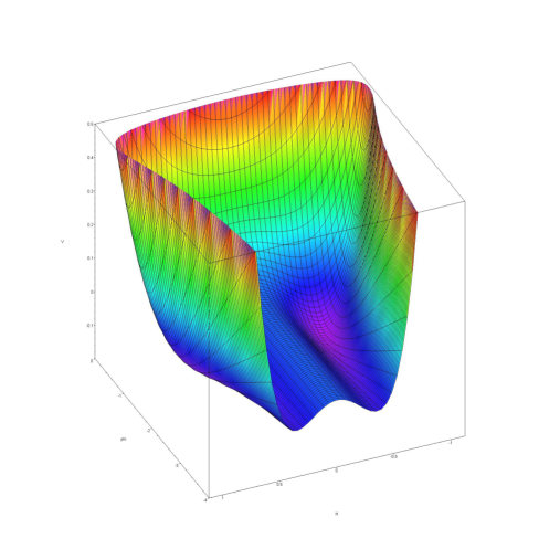
Figure 1: The effective Higgs-dilaton potential in the vicinity of its two symmetric local minimums: $H^{2}=H^{2}_{m}=0.31$ and $\phi=\phi_{m}=-1.38$. Black lines represent the sections of the plot of the potential by the surfaces of constant $\phi$ and constant $H$. Parameters are taken as follows: $A=1$, $B=2.1$, $C=1$, $E=-1$.

Evidently the phase transition point during evolution appears for $\phi_{crit}=(1/2)\ln(-E/B)<\phi_{in}$. It can be shown that $\phi_{fin}<\phi_{crit}<0$ and therefore $B+E>0$. We remark that the latter inequality entails $|E_{min}|>|E|$ . As well in this case for $\phi_{in}\leq 0$ the Higgs potential is bounded below for any value of Higgs fields.

By the way we notice that due to (4),(64), critical point $\phi_{c}$ coincides with $\phi_{0}$ and the latter comes from the invariant action $\hat{W}_{\mathrm{inv}}$ (56). Thereby the requirement $\phi_{c}=\phi_{0}<0$ means that the invariant potential $-C\phi_{0}H^{4}$, corresponding to $\hat{W}_{\mathrm{inv}}$ is bounded bellow.

We summarize our finding in Fig. 1. One can see that for the values of $\phi\simeq 0$ there is only one minimum of the function $V(H)|_{\phi=fixed}$ at $H=0$. When we get closer to $\phi_{m}$ crossing $\phi_{crit}$, the phase transition occurs, and every function $V(H)|_{\phi=fixed}$ has two symmetric minimums. The section of this three-dimensional plot in the initial point $\phi_{in}=0$ is shown in Fig. 2 and reveals the absolute minimum in Higgs fields.

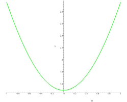
Figure 2: $V(H)$ at the fixed value of $\phi=\phi_{in}=-0.1$ i.e. the profile of the potential in the symmetric phase. $A=1$, $B=2.1$, $C=1$, $E=-1$.

Such a choice of the parameters provides an existence of the local minimum in the late stage of the universe evolution at $\phi_{m}=-1.38$ and $H_{m}^{2}=0.31$. So in the Higgs phase ($\phi=\phi_{m}$) one has the following potential behavior, $V(H,\phi_{m})=0.0039-0.87H^{2}+1.38H^{4}$, see Fig. 3.

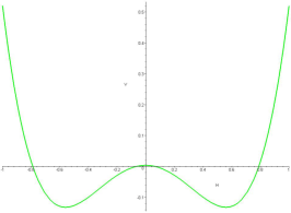
Figure 3: $V(H)$ at the fixed value of $\phi=\phi_{m}=-1.38$ i.e. the profile of the potential in the Higgs phase. $A=1$, $B=2.1$, $C=1$, $E=-1$.

In the next Fig. 4

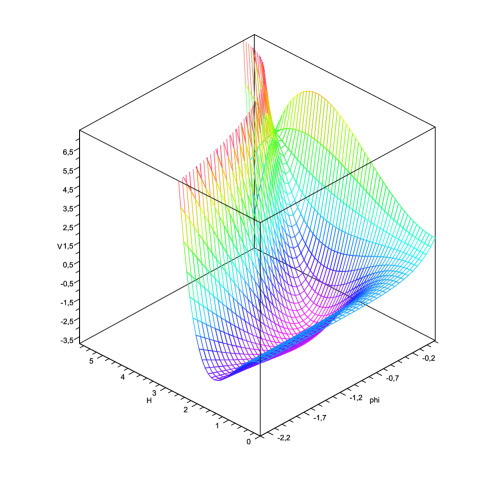
Figure 4: The similar effective Higgs-dilaton potential in the vicinity of its local minimum: $H=H_{m}=2.29$ and $\phi=\phi_{m}=-0.72$ chosen to display the saddle point. Colored lines represent the sections of the plot of the potential by the surfaces of constant $\phi$ and constant $H$. Parameters are taken as follows: $A=1$, $B=2.1$, $C=0.2$, $E=-2$.

another view on the plot for effective potential is taken in order to demonstrate that the saddle point is aside of the steepest descend path.

7.3 Remark.

Let us notice, that one is not allowed to identify the minimal value of HD-potential $V_{min}$ with cosmological constant, because at $A,B,C>0,-B<E<0$ we can easily prove, that $V_{min}<0$.

Indeed, our potential (60) satisfies the following relation:

$$V=\frac{1}{4}\left(\frac{\partial V}{\partial\phi}+H\frac{\partial V}{\partial H}\right)+\frac{H^{2}}{4}\left(CH^{2}+2E\right)+V_{0}$$ (77)

and thereby its minimal value is given by

$$V_{m}=V_{0}+\frac{H_{m}^{2}}{4}\left(CH^{2}+2E\right).$$ (78)

For a given value of the Higgs v.e.v. $H_{m}\equiv\eta_{fin}e^{2\phi_{fin}}$ one can present the coefficient $E$ in the form

$$E=H_{m}^{2}\cdot CW_{-1}\left(\frac{Ee^{-\frac{B}{C\eta_{fin}}}}{C\eta_{fin}}\right).$$ (79)

Substituting (79) into (78) we have:

$$V_{m}=V_{0}+\frac{CH^{4}}{4}\left(1+2W_{-1}\left(\frac{Ee^{-\frac{B}{C\eta_{fin}}}}{C\eta_{fin}}\right)\right)$$ (80)

and taking into account, that $V_{0}<0$, $W_{-1}\leq-1$ we finally obtain:

$$V_{m}<-\frac{CH_{m}^{4}}{4}<0.$$ (81)

Anyway we suppose, that the observed cosmological constant is generated by both visible and dark matter, and only visible matter participates in the dilaton - bosonization process considered above and hence $V_{m}$ can be identified with (negative) contribution to the total (positive) cosmological constant.

Let’s use first the metric $g_{\mu\nu}$ as a background one and therefore independently in the dark and visible sectors,

$$Z_{\mathrm{total}}(g_{\mu\nu})=Z_{\mathrm{dark}}(g_{\mu\nu})\cdot Z_{\mathrm{SM}}(\tilde{g}_{\mu\nu},H)\Big{|}_{\tilde{g}_{\mu\nu}=g_{\mu\nu}}.$$

Performing bosonization $\tilde{g}_{\mu\nu}\to\tilde{g}_{\mu\nu}\exp(2\phi);\ H\to H\exp(-\phi)$ in the SM sector only one finds,

$$Z_{\mathrm{SM}}(\tilde{g}_{\mu\nu},H)=\hat{Z}_{\mathrm{inv}}(\tilde{g}_{\mu\nu},H)\int d\phi\,e^{-S_{\mathrm{\mathrm{coll}}}(\tilde{g}_{\mu\nu},H,\phi)}\simeq\int d\phi e^{-\int d^{4}x\sqrt{-g}V(\tilde{g}_{\mu\nu},H,\phi)}.$$

The total cosmological generating functional is produced after averaging over gravity, i.e. over the metrics,

$$Z_{\mathrm{cosm}}=\int{\cal D}g_{\mu\nu}\times[\mathrm{gauge\ fixing}]\times e^{-W_{grav}(g)}Z_{\mathrm{dark}}(g_{\mu\nu})\cdot Z_{\mathrm{SM}}(g_{\mu\nu},H).$$

The latter integral in the vacuum energy approximation for matter fields entails the determination of the cosmological constant,

$$Z_{\mathrm{cosm}}\sim\int{\cal D}g_{\mu\nu}\times[\mathrm{gauge\ fixing}]\times e^{-W_{grav}(g)-\int d^{4}x\sqrt{-g}\frac{\Lambda_{cosm}}{8\pi G_{N}}},$$

which evidently consists of,

$$\frac{\Lambda_{cosm}}{8\pi G_{N}}=V_{0,SM}+V_{0,\mathrm{dark}},\quad\int d^{4}x\sqrt{-g}V_{0,\mathrm{dark}}\simeq-\log Z_{\mathrm{dark}}.$$

All formulas are referred to the Euclidean space-time and can be re-written easily for the Minkowski one.

8 Conclusions

In this paper we have seen how the bosonic spectral action emerges form the fermionic action and Weyl anomaly via the renormalization group flow. In this sense we can say that the bosonic degrees of freedom are induced by the fermionic ones. The procedure followed is spectral and therefore well suited for the noncommutative approach to the standard model. The action emerges, in case of the presence of a fundamental scale, and therefore of a non Weyl invariant fundamental theory, in terms of a composite dilaton.

What we find particularly encouraging is the fact that, at the level of effective potential, the theory gives rise to a Higgs-dilaton potential with desirable qualitative features, i.e. the presence of both a broken and an unbroken phase, and the possibility to roll form the latter to the former. We did so using just the bare essential ingredients of the spectral action, and therefore the result, while necessarily generic and qualitative, are to a large extend independent on the details of the model. We see a certain relevance of the Higgs-dilaton potential of our type for realization of the Higgs field assisted inflation and further stages of the Universe evolution undertaken in [34, 35]. A refinement of this work taking other degrees of freedom into account is possible, and partially under way.

A Appendix

In this appendix we show why $W_{\mathrm{inv}}$ is proportional to $H^{4}$. In the approximations taken, when all the fields do not depend on the space-time coordinates one may infer (up to the additional terms, proportional to $H^{4}$) the dependence on the Higgs field of the initial effective potential $W$, related to $Z$ (9), based on the requirement, that $Z_{\mathrm{inv}}$ (19) is invariant under the Weyl transformation (8).

Since we are interested in the form of the effective Higgs potential and ignore all derivative terms, one can write $Z(H)$ instead of $Z(D)$, and consider ordinary integrals over $\phi$ instead of functional.

We have seen (25), that the invariant partition function can be rewritten as:

$$Z_{\mathrm{inv}}(H)=Z(H)\cdot Z_{\mathrm{anom}}(H)=e^{-W(H)}\cdot\int d\phi e^{-S_{\mathrm{anom}}(\phi,H)},$$ (1)

where $S_{\mathrm{anom}}\equiv\int d^{4}x\sqrt{|g|}V_{\mathrm{anom}}$ and due to (48) and (59):

$$V_{\mathrm{anom}}=-V_{\mathrm{coll}}=-\int d^{4}x\sqrt{|g|}\left\{\tilde{A}\left(e^{4\phi}-1\right)+\tilde{B}H^{2}\left(e^{2\phi}-1\right)-C\phi H^{4}\right\},$$ (2)

Where

$$\tilde{A} = \frac{45}{8\pi^{2}}\frac{\Lambda^{4}}{8}\left(2\log\frac{\Lambda^{2}}{\mu^{2}}-1\right),$$ (3)

$$\tilde{B} = \frac{3y^{2}}{2\pi^{2}}\frac{\Lambda^{2}}{2}\left(1-\log\frac{\Lambda^{2}}{\mu^{2}}\right),$$ (4)

$$C = \frac{3z^{2}}{4\pi^{2}}.$$ (5)

Notice, that we can perform integration over $\phi$ in 1 via the Laplace method. Indeed, in our approximation we neglect all the (covariant) derivatives, thats why $S_{\mathrm{anom}}$ is proportional to the volume $vol$ of space-time (we have an infrared cutoff implicit in the theory).

$$\int d\phi e^{-(vol)\cdot V_{\mathrm{anom}}(H,\phi)} \simeq \sqrt{\frac{2\pi}{vol\cdot\frac{\partial^{2}V_{\mathrm{anom}}(H,\phi_{min})}{\partial\phi^{2}}}}e^{-(vol)\cdot V_{\mathrm{anom}}(H,\phi_{min})}$$ (6)

$$= e^{-(vol)\cdot\left(V_{\mathrm{anom}}(H,\phi_{min})+\frac{O(\ln{(vol)})}{vol}\right)}.$$

Taking into account, that $vol$ goes to infinity we must take into account only the leading term in the exponent. Thereby one can finally write:

$$W_{\mathrm{anom}}(H)\equiv e^{-W_{\mathrm{anom}}(H)},~{}~{}~{}W_{\mathrm{anom}}\equiv{\int d^{4}x\sqrt{|g|}V_{\mathrm{anom}}(H,\phi=\phi_{min}(H))}.$$ (7)

For a fixed value of $H$ the function $V_{\mathrm{anom}}(\phi,H=fixed)$ has a local minimum at the point:

$$\phi_{min}(H)=\frac{1}{2}\ln\left({\frac{\left(\tilde{B}+\sqrt{{\tilde{B}}^{2}+4\,\tilde{A}C}\right)H^{2}}{-4\tilde{A}}}\right),$$ (8)

if and only if $\tilde{A}<0,~{}\tilde{B}>0$. Thereby we have the following expression for $V_{\mathrm{anom}}$:

$$V_{\mathrm{anom}}=\tilde{A}+\tilde{B}H^{2}+\frac{CH^{2}}{2}\ln\left({\frac{\left(\tilde{B}+\sqrt{{\tilde{B}}^{2}+4\,\tilde{A}C}\right)H^{2}}{-4\tilde{A}}}\right)+H^{4}\cdot const(A,B,C).$$ (9)

By the construction we know, that $Z_{\mathrm{inv}}$ is unchanged under the transformation 8. It means, that $W_{\mathrm{inv}}(H)=W(H)+W_{inv)(H)}$ must be invariant under the transformation

$$g_{\mu\nu}\rightarrow e^{2\phi}g_{\mu\nu},\\ H\rightarrow e^{-\phi}H.$$

Thereby we have the following functional equation for $V(H)$

$$V(e^{-\phi}H)+V_{\mathrm{anom}}(e^{-\phi}H)=e^{-4\phi}(V(H)+V_{\mathrm{anom}}(H)).$$ (10)

One can easily see, that the most general solution of the 10 is given by

$$V=-\tilde{A}-\tilde{B}H^{2}-\frac{CH^{2}}{2}\ln\left(\frac{H^{2}}{\tilde{\mu}}\right),$$ (11)

where $\tilde{\mu}$ is an integration (dimensionful) constant. Finally we obtain from (11) and (9) (as we expected):

$$V_{\mathrm{inv}}=V+V_{\mathrm{anom}}=\tilde{\gamma}H^{4},$$ (12)

with some (undefined at this stage) constant $\gamma$. We emphasize, that the potential $V$ given by (11) has a local minimum at $\tilde{A}<0,\tilde{B}>0$, but after averaging over dilatations the minimum disappears.

We also notice, that we can perform similar integration via the Laplace method in the (57). In this case minimum of $V_{\mathrm{coll}}=-V_{\mathrm{anom}}$ is of our interest, i.e. maximum of $V_{\mathrm{anom}}$. The latter is given by

$$\phi_{max}(H)=\frac{1}{2}\ln\left({\frac{\left(\tilde{B}-\sqrt{{\tilde{B}}^{2}+4\,\tilde{A}C}\right)H^{2}}{-4\tilde{A}}}\right),$$ (13)

and it exists both for positive and negative signs of $\tilde{A}$, and $\tilde{B}>0$. In this case one has the same expression (11) for $V$, which is defined, we remind, up to the invariant term, proportional to $H^{4}$. In this sense the point of view taken in this paper, that is of a partition function which is not Weyl invariant, and that of reference [7], are not in fundamental contradiction..

References

- [1] A. Connes, Noncommutative Geometry, Academic Press, 1984.
- [2] A. Connes and J. Lott, “Particle Models and Noncommutative Geometry (Expanded Version),” Nucl. Phys. Proc. Suppl. 18B (1991) 29.
- [3] A. H. Chamseddine and A. Connes, “The spectral action principle,” Commun. Math. Phys. 186, 731 (1997) [arXiv:hep-th/9606001].
- [4] A. H. Chamseddine, A. Connes and M. Marcolli, “Gravity and the standard model with neutrino mixing,” Adv. Theor. Math. Phys. 11 (2007) 991 [arXiv:hep-th/0610241].
- [5] A. D. Sakharov, “Vacuum quantum fluctuations in curved space and the theory of gravitation,” Sov. Phys. Dokl. 12 (1968) 1040 [Dokl. Akad. Nauk Ser. Fiz. 177 (1967 SOPUA,34,394.1991 GRGVA,32,365-367.2000) 70].
- [6] M. Visser, “Sakharov’s induced gravity: A modern perspective,” Mod. Phys. Lett. A 17 (2002) 977 [arXiv:gr-qc/0204062].
- [7] A. A. Andrianov and F. Lizzi, “Bosonic Spectral Action Induced from Anomaly Cancelation,” JHEP 1005 (2010) 057 [arXiv:1001.2036 [hep-th]].
- [8] A. A. Andrianov, M. A. Kurkov and F. Lizzi, “Spectral Action from Anomalies,”, Corfù Summer Institute on Elementary Particles and Physics - Workshop on Non Commutative Field Theory and Gravity, September 2010 Corfù Greece, arXiv:1103.0478 [hep-th].
- [9] K. Fujikawa, H. Suzuki, Path Integrals And Quantum Anomalies, Oxford university Press, 2004.
- [10] A. H. Chamseddine and A. Connes, “Scale invariance in the spectral action,” J. Math. Phys. 47 (2006) 063504 [arXiv:hep-th/0512169].
- [11] A. A. Andrianov and Yu. V. Novozhilov, “Gauge Fields and Correspondence Principle,” Theor. Math. Phys. 67, 448 (1986) [Teor. Mat. Fiz. 67, 198 (1986)].
- [12] F. Lizzi, G. Mangano, G. Miele and G. Sparano, “Fermion Hilbert space and fermion doubling in the noncommutative geometry approach to gauge theories,” Phys. Rev. D 55, 6357 (1997) [arXiv:hep-th/9610035].
- [13] J. M. Gracia-Bondia, B. Iochum and T. Schucker, “The standard model in noncommutative geometry and fermion doubling,” Phys. Lett. B 416, 123 (1998) [arXiv:hep-th/9709145].
- [14] A. H. Chamseddine and A. Connes, “Space-Time from the spectral point of view,” arXiv:1008.0985 [hep-th].
- [15] T. Schucker, “Forces from Connes’ geometry,” Lect. Notes Phys. 659, 285 (2005) [arXiv:hep-th/0111236].
- [16] A. A. Andrianov, L. Bonora and R. Gamboa-Saravi, “Regularized Functional Integral For Fermions And Anomalies,” Phys. Rev. D 26, 2821 (1982).
- [17] A. A. Andrianov and L. Bonora, “Finite - Mode Regularization Of The Fermion Functional Integral,” Nucl. Phys. B 233, 232 (1984).
- [18] A. A. Andrianov and L. Bonora, “Finite Mode Regularization Of The Fermion Functional Integral. 2,” Nucl. Phys. B 233, 247 (1984).
- [19] A. A. Andrianov, V. A. Andrianov, V. Y. Novozhilov and Yu. V. Novozhilov, “Joint Chiral and Conformal Bosonization in QCD and the Linear Sigma Model,” Phys. Lett. B 186 (1987) 401.
- [20] Y. V. Novozhilov and D. V. Vassilevich, “Induced Quantum Conformal Gravity,” Phys. Lett. B 220 (1989) 36.
- [21] J. M. G. Fell and R. S. Doran, Representations of ∗-Algebras, Locally Compact Groups and Banach ∗-Algebraic Bundles, Academic Press, (1988).
- [22] J.M. Gracia-Bondia, J.C. Varilly, H. Figueroa, Elements of Noncommutative Geometry, Birkhauser, 2000.
- [23] G. Landi, An Introduction to Noncommutative Spaces and their Geometries, Springer Lecture Notes in Physics 51, Springer Verlag (Berlin Heidelberg) 1997. arXiv:hep-th/9701078.
- [24] J. Madore, “An Introduction To Noncommutative Differential Geometry and its Physical Applications,” Lond. Math. Soc. Lect. Note Ser. 257 (2000) 1.
- [25] J. Madore, “Kaluza-Klein Aspects Of Noncommutative Geometry,” In *Chester 1988, Proceedings, Differential geometric methods in theoretical physics* 243-252.
- [26] M. Dubois-Violette, R. Kerner and J. Madore, “Noncommutative Differential Geometry Of Matrix Algebras,” J. Math. Phys. 31 (1990) 316.
- [27] A. Sitarz, “Spectral action and neutrino mass,” Europhys. Lett. 86 (2009) 10007 [arXiv:0808.4127 [math-ph]].
- [28] J. W. Barrett, “State sum models, induced gravity and the spectral action,” arXiv:1101.6078 [hep-th].
- [29] D. V. Vassilevich, “Heat kernel expansion: User’s manual,” Phys. Rept. 388, 279 (2003) [arXiv:hep-th/0306138].
- [30] W. Nelson and M. Sakellariadou, “Cosmology and the Noncommutative approach to the Standard Model,” arXiv:0812.1657 [hep-th].
- [31] M. Marcolli and E. Pierpaoli, “Early Universe models from Noncommutative Geometry,” arXiv:0908.3683 [hep-th].
- [32] http://en.wikipedia.org/wiki/Lambertfunction .
- [33] Lambert, J. H. ”Observations variae in Mathesin Puram.” Acta Helvetica, physico-mathematico-anatomico-botanico-medica 3, 128-168, 1758. Euler, L. ”De serie Lambertina Plurimisque eius insignibus proprietatibus.” Acta Acad. Scient. Petropol. 2, 29-51, 1783.
-
[34]
F. L. Bezrukov and M. Shaposhnikov,
“The Standard Model Higgs boson as the inflaton,
Phys. Lett. B 659, 703 (2008)
[arXiv:0710.3755 [hep-th]];
F. Bezrukov, A. Magnin, M. Shaposhnikov and S. Sibiryakov, “Higgs inflation: consistency and generalisations,” JHEP 1101, 016 (2011) [arXiv:1008.5157 [hep-ph]]. - [35] A. O. Barvinsky, A. Y. Kamenshchik, C. Kiefer and C. F. Steinwachs, “Tunneling cosmological state revisited: Origin of inflation with a non-minimally coupled Standard Model Higgs inflaton, Phys. Rev. D 81, 043530 (2010) [arXiv:0911.1408 [hep-th]].