Nematic phase without Heisenberg physics in FeAs planes

Abstract

We use Monte Carlo simulations and analytical arguments to analyze a frustrated Ising model with nearest neighbour antiferromagnetic coupling $J_{1}$ and next nearest neighbour coupling $J_{2}$. The model is inspired on the physics of pnictide superconductors and to some extent we argue that it can be more representative of this physics than the Heisenberg counterpart. Parameters are chosen such that the ground state is a columnar or striped state, as observed experimentally, but is close to the transition to the simple Néel ordered antiferromagnetic state $R=J_{2}/|J_{1}|\gtrsim 0.5$. We find that a nematic phase is induced close to $R=0.5$ by finite size effects and argue that this explains experiments in imperfect samples which find a more robust nematic state as the quality of the sample decreases [A. Jesche et al., Phys. Rev. B 81, 134525 (2010)]. Including the effect of a weak coupling with the lattice we find that a structural transition occurs associated with a nematic phase, with a magnetic transition occurring at a lower temperature. These two transitions merge into a single structural and magnetic transition with a stronger first-order character for larger spin-lattice couplings. These two situations are in agreement with the different phenomenologies found in different families of pnictides.

I Introduction

The FeAs high-Tc materials kamihara ; rotter are a very interesting new playground to study the interplay between lattice, magnetism and superconductivity. Quite generically undoped or slightly doped samples show a magnetic phase which breaks the $C_{4}$ symmetry of the lattice, consisting of magnetic moments aligned ferromagnetically on one direction and antiferromagnetically in the other direction. This “columnar” or “spin-stripe” phase is accompanied by an orthorhombic distortion of the high temperature tetragonal lattice.

From symmetry considerations it is quite natural to assume that the structural transition from the high temperature tetragonal phase to the orthorhombic phase is driven by the magnetism. However ‘1111’ materials like LaOFeAsdelaCruz2008Magnetic display the structural transition at a higher temperature than the magnetic transition. This has led some authors to propose that the structural transition drives the magnetism. Even more surprising is the fact that the temperature splitting between structural and magnetic transitions decreases upon increasing the sample qualityJesche2010Coupling and the transport anisotropy is reduced.liang

The stripe-magnetic phase, breaking both the $C_{4}$ symmetry and the translation symmetry can be called “smectic”, in analogy with the crystal phase that elongated molecules form in liquid crystals. However in the last few years the question has emerged whether a “nematic” phase can also occur in these systems. The term “nematic”, which is also borrowed from the field of liquid crystals, indicates a phase where the rotational symmetry is broken, while the translational symmetry is fully preserved. In the pnictide case, for instance, the square lattice $C_{4}$ symmetry of the FeAs layers in the tetragonal phase could be reduced to $C_{2}$ by the occurrence of a purely magnetic nematic phase. In turn this nematic state could involve an interplay between structural and magnetic properties giving rise to structural and lattice signatures even in the absence of a “smectic” magnetic order. This issue not only has been addressed from the theoretical point of view Fang2008Theory ; xusachdev ; Vojta2009Lattice ; fernandes2 , but increasing evidence is now experimentally emerging of a nematic state above the magnetic transition in pnictides. Scanning tunnelling microscopy studies detect quasiparticle electronic states having a reduced $C_{2}$ symmetry zhou as well as local anisotropies chuang , transport experiments in detwinned 122 crystals find an in-plane anisotropy, which cannot be attributed to lattice distortions only chu ; tanatar , while optical experiments find anisotropic mid-infrared spectra dusza . If such nematic phase exists, the coupling between the magnetic nematic state and the lattice would naturally account for the occurrence in some materials (like 1111 or Ba(Fe_1-xCo_x)₂As₂) of the tetragonal-orthorhombic transition at a higher temperature than the magnetic transition. The coupling between nematicity and lattice has also been taken as a possible explanation for changes in elastic properties observed by ultrasound spectroscopy in FeAs systems fernandes1 , and the suppression of orthorombicity in the superconducting phase nandi .

An important question is if an electronic nematic phase drives the lattice distortion or vice versa. The split transitions occur only when the thermal transition is continuous or very close to continuous. On the other hand most ‘122’ materials like SrFe₂As₂Krellner2008Magnetic show a first-order transition in which simultaneously the structural and the magnetic order parameter become non-zero.

The more straightforward explanation for nematic phases starts from a two-dimensional frustrated Heisenberg modelFang2008Theory and is based on theoretical results that dates back two decades.larkin This explanation relays on the order by disorder mechanism by which the degeneracy of the frustrated Heisenberg model at the classical level is broken by thermal and quantum fluctuations. As a consequence a nematic phase is stabilized which has Ising symmetry. In two dimensions antiferromagnetic (AF) long-range order can only occur at zero temperature while the nematic phase, belonging to the Ising universality class, can occur at finite temperatures thus a large region of temperatures exists where the system is in a nematic phase. Interlayer coupling stabilizes a three dimensional AF state but always with a magnetic transition occurring at a lower temperature than the Ising nematic transition.Fang2008Theory

While this explanation is very appealing it is worth to examine whether the Heisenberg physics is really necessary and if there can be other mechanism by which nematic phases can be stabilized. One motivation to do so is that the region where the Heisenberg physics is relevant can be quite narrow around the Néel temperature. Indeed stoichiometric FeAs materials have small magnetic moments and are metallic which indicates rather itinerant magnetismZhang2010Itinerant . The magnetism thus is rather collective which means that a given site does not interact only with the neighbors but with several sites over a coherence distance $\xi_{0}\gg a$, with $a$ the lattice spacing. To observe Heisenberg-like critical fluctuations the magnetic correlation length $\xi$ has to exceed $\xi_{0}$ which occurs only very close to the magnetic critical temperature. If $\xi_{0}$ is sufficiently large a small Ising like anisotropy or a three dimensional coupling will make the 2D Heisenberg physics and the Goldstone modes rather irrelevant. One way to suppress from the start the presence of the Goldstone modes and have a finite critical temperature is to consider Ising spins.

In this work we study a frustrated two-dimensional Ising model. For simplicity we assume localized spins which interact through effective nearest-neighbor and next-nearest-neighbor antiferromagnetic interactions ($J_{1}>0$ and $J_{2}>0$ respectively) (see, e.g. Ref. Yildirim2008Origin, ). We thus obtain a frustrated Ising model without any interaction between the spins and the lattice and only at a later stage we will introduce a spin-lattice coupling. The model’s phase diagram is studied using Monte Carlo simulations and finite size analysis.

This model is interesting in its own and although its magnetic properties have already been extensively investigatedLopez1993Firstorder , our analysis will evidentiate new features and it will find interesting connections with the real pnictide systems. We show that the critical behavior corresponds closely to a 4-component Potts model.

For $0<R=J_{2}/|J_{1}|<0.5$, it is well known that there is a second-order transition toward a low temperature Néel antiferromagnetic phase. For $R>0.5$ the system shows a magnetic transition toward the “spin-stripe” phase observed in FeAs planes and mentioned above. While in other cases, like in manganites, this antiferromagnetic spin configuration has been named c-type antiferromagnetism, we will keep the “spin-stripe” phase nomenclature as usual in the pnictide field.

Our analysis aims to explore the possibility of having nematic phases when all the Heisenberg physics is suppressed. Although the model is very simplified we show below that it explains well several aspect of the phenomenology of FeAs planes. In particular we find that nematic phases can be stabilized at finite temperatures by finite size effects. We argue that such effect can explain the larger tendency of “bad samples” to display nematic phases.

The paper is structured as follows. In Sect. II we introduce the model and the technical framework to solve it. In Sect. III we report the results in the absence of the spin-lattice coupling, which is instead introduced in Sect. IV. Our concluding remarks are in Sect. V.

II Model and methods

We consider a two-dimensional frustrated Ising model with antiferromagnetic nearest-neighbour (nn) and next-nearest-neighbor (nnn) interactions. The Hamiltonian of the model reads

$$H_{M}(\{\sigma_{i}\}) = \sum_{i=1}^{N}\sum_{\delta=x,y}J_{1}\,\sigma_{i}\sigma_{i+\delta}$$ (1)

$$+\sum_{i=1}^{N}\sum_{\eta=x+y,-x+y}J_{2}\,\sigma_{i}\sigma_{i+\eta},$$

with $J_{1}$ and $J_{2}$ both positive. The notation $i+x$ ($i+x+y$) indicates the first (second) neighbour of site $i$ in the $x$ ($x+y$) direction. One can use a canonical transformation $\sigma_{i}\rightarrow(-1)^{x_{i}+y_{i}}\sigma_{i}$ to change the sign of the first term. This means that since the model is classical it is fully equivalent to a nn ferromagnetic model with AF frustration among nnn which has been extensively studied in the literatureLopez1993Firstorder .

If frustration is strong enough ($R>0.5$), the ground state is given by a spin-stripe configuration. This configuration breaks both rotational symmetry and traslational symmetry in one direction. This state is characterized by a staggered magnetization with $(\pi,0)$ or $(0,\pi)$ wave vectors, which, for one configuration, is defined by

$$m_{(\pi,0)}=\frac{1}{N}\sum_{j}\sigma_{j}\,{(-1)}^{x_{j}};$$ (2a)

$$m_{(0,\pi)}=\frac{1}{N}\sum_{j}\sigma_{j}\,{(-1)}^{y_{j}},$$ (2b)

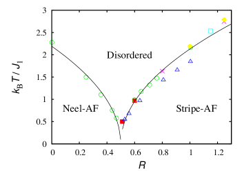
We notice that at $T=0$, for a given orientation of the spin stripes, only one of the two staggered magnetizations is non zero. The sign of the two parameters depends on the position of the spin up stripes (odd or even rows or columns). In Fig.1 we report the phase diagram of the model in Eq.(1) as obtained by Morán-López et al.Lopez1993Firstorder studying the equivalent nn ferromagnetic version. Here we have added two points obtained from our MC calculations. More detailed data including nematic and lattice effects will be shown below. In Ref. Lopez1993Firstorder, it was found that the transition toward the spin-stripe phase is weakly first-order up to a tricritical point at $R=1.144$. For higher values of $R$ the transition becomes of the second-order.

Figure 1: (Color online) Phase diagram of the system. Each point represents the critical temperature for a given value of $R$, and the types of point depends on the different methods used to compute them. Empty circles (green online) have been obtained with Monte Carlo; empty triangles (blue online) have been obtained with real space renormalization group; crosses (purpleonline) indicate have been obtained with Monte Carlo renormalization group; the solid (yellow online) circles have been obtained with series expansion. The open square (light blue online) marks the tricritical point at $R=1.144$Lopez1993Firstorder . The solid square (red online) mark the critical temperature values obtained with our MC simulations. The model studied in Ref. Lopez1993Firstorder, considers ferromagnetic nn interactions so that the ordered phase up to $R=0.5$ should more precisely be named “Néel-F”.

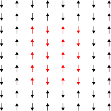
In Fig. 2 we show a domain of the perfect stripe order in which the directionality is preserved but the phase of the AF changes by $\pi$. At finite temperatures it can happen that domains of this kind are preferentially excited destroying the long-range magnetic order but still breaking $C_{4}$ rotational symmetry so that the system reaches a nematic state.

Figure 2: (Color online) Illustration of a spin domain (gray arrows, red online), in which the staggered magnetization in x direction has opposite sign with respect to the embedding cluster (black arrows).

Following Ref. Vojta2009Lattice, we define a nematic magnetization which measures the global breaking of $C_{4}$ symmetry and which for one configuration reads,

$$m_{\phi}=\frac{\sum_{i}\phi_{i}}{N}.$$ (3)

Here the local nematic parameter $\phi_{i}$ is defined by

$$\phi_{i}=\frac{1}{2}\sigma_{i}(\sigma_{i+x}-\sigma_{i+y}).$$ (4)

The magnetic and nematic order parameters are defined as the thermal averages $\langle...\rangle$ of Eqs. (2a),(2b),(3). The range of all these three parameters is $[-1:1]$.

The “nematic phase” is characterized by finite values of the nematic magnetization, consequence of the break of the rotational symmetry $C_{4}$, but vanishing values of the staggered magnetization. It is customary to call $\langle m_{\phi}\rangle$ the nematic order parameterVojta2009Lattice and we follow this convention here, although it is different from zero also in the spin-stripe or smectic phase which, strictly speaking, are not nematic phases. The sign of $\langle m_{\phi}\rangle$ depends on the preferred orientation of the spin stripes. Table II summarizes the above discussion of the order parameters.

	$\langle m_{(\pi,0)}\rangle$, $\langle m_{(0,\pi)}\rangle$	$\langle m_{\phi}\rangle$
Disorder	0	0
Magnetic phase	$\neq 0$	$\neq 0$
Nematic phase	0	$\neq 0$

To numerically implement our analysis we define a square matrix (that is our lattice), every element of which may assume the values $\pm 1$, according to the up or down orientation of the spin on the site. Physical quantities like staggered magnetizations, nematic order parameter, spatial correlation functions and susceptibilities, are calculated using the MC methodNewman1999Monte ; Katzgraber2010Introduction . This method exploits the Metropolis algorithm to generate, in a random way, a chain of states (called “Markov chain”), which are distributed according to the Boltzmann distribution function. Thus the MC procedure is able to simulate the thermal fluctuations of the physical quantities upon exploring the phase space with a discrete time evolution consisting of subsequent MC steps [thus our time unit is a MC Step (MCS)]. The thermal averages become averages over the MC evolution after a suitable thermalization of the system. We use a thermalization time constituted by $2000\times n$ MCS (where $n$ is the total number of the spins of our system). Furthermore each point of the Markov chain must be generated after some MCS from the previous one so that each measure becomes uncorrelated from the others. Therefore between two measures we wait a time longer than the autocorrelation time. In our specific case this waiting time is chosen to be $500\times n$ MCS. Analyzing the time fluctuations of the observables, we have verified that these choices of thermalization and autocorrelation time are optimal to have reliable measures.

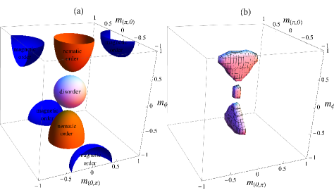
Each configuration can be characterized by the instantaneous value of the three magnetizations $\left(m_{(\pi,0)},m_{(0,\pi)},m_{\phi}\right)$ defining a point in a three dimensional space. Fig. 3(a) is a schematic representation of the regions where the points corresponding to instantaneous configurations should be more dense in each one of the phases summarized in Table II.

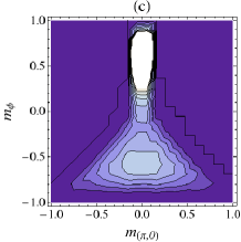
In order to characterize the different phases we compute the threedimensional (3D) density distribution of points at each temperature of the simulation. This distribution can be visualized either by projection on one plane (Fig. 3(c)) or by plotting 2D isosurface with a given number of points per unit volume (Fig. 3(b)). The points are expected to be distributed with a Boltzmann weight $\exp\left[-F(m_{(\pi,0)},m_{(0,\pi)},m_{\phi})/k_{B}T\right]$ thus higher density of points corresponds to the lower free energy $F$ and indicates the most stable phase. As it will be discussed in greater detail in the next section, the example in Fig. 3(b,c)orresponds to the nematic phase. Since the distribution are rather flat for a given sign of the nematic order parameter, the two-dimensional plots like the one of Fig. 3(c) allows to visualize the competition between the nematic and the ordered phase. Similar information can be cast in the form of a scatter plot as in the example of Fig. 6 below. Notice that the competition between the nematic and the disordered phase are not well characterized by this method. In any case we have checked all our results with the more rigorous 3D visualization method. Specific details for each phase are discussed in next Section.

Due to the symmetries in the Hamiltonian for a generic point $\left(m_{(\pi,0)},m_{(0,\pi)},m_{\phi}\right)$ there are 7 other points which correspond to distinct configurations with the same energy. The symmetries are the reflection around the $m_{(\pi,0)}=0$ and $m_{(0,\pi)}=0$ planes and the reflection with respect to the $m_{\phi}=0$ plane followed by a $90^{\circ}$ rotation respect to the $m_{\phi}$ axis. This last rotation is due to the fact that the sign of $m_{\phi}$ is linked to the direction of the stripes. With these symmetries for each point obtained in the simulations we obtain 7 other symmetry-related points increasing the statistic and producing perfectly symmetric distributions as expected for non symmetrized simulations performed for very long times.

Figure 3: (Color online) Phase space of the order parameters. (a) the spheres or ellipsoids schematically describe the different phases of the system. When the order parameter is distributed inside the central sphere the system is disordered. An order parameter inside the lightly shaded (orange online) ellipsoid indicates robust nematic order, while when the order parameters are inside the darker shaded (blue online) ellipsoids a magnetic state is realized. (b) Example of a MC simulation on a $50\times 50$ lattice for $R=0.51$ and $k_{B}T/J_{1}=0.52$. Statistically independent points where binned according to the value of the 3D magnetization $\left(m_{(\pi,0)},m_{(0,\pi)},m_{\phi}\right)$ in cells of size $0.1\times 0.1\times 0.1$. We show an isosurface with 500 points per bin. (c) Contour plot of the distribution projected onto the $m_{(0,\pi)}=0$ plane with bins of size $0.1\times 0.1$. The bins with higher counts are the most bright.

III Results

To characterize the transitions to the ordered states, we determine the critical indices of the magnetic and nematic transitions using the Finite Size Scaling techniqueNewman1999Monte ; Binder2002Monte . Using our MC simulation, we calculate the temperature dependence of the interesting physical quantities of the system for three different lattice sizes: $10\times 10$, $24\times 24$, $50\times 50$, using a value of $R$ not too close to the $T=0$ critical point $R=0.50$. Thus we choose $R=0.60$. Although for this value of $R$, the magnetic transition is of first-orderLopez1993Firstorder , since the transition is ‘weakly’ of the first-order, we can still compute “critical indexes” describing the substantial growth of the various susceptibilities near the transition. We first calculate the temperature and size dependence of the Binder CumulantBinder2002Monte

$$U_{4}\left[m\right]=1-\frac{\langle m^{4}\rangle}{3\,{\langle m^{2}\rangle}^{2}},$$ (5)

where $\langle m\rangle$ is the thermal average of the parameter we are interesting in (in our case the staggered magnetizations or the nematic one). The temperature at which the value of $U_{4}$ is the same for the three different lattice size defines the critical temperature of the transition. We show in Fig.4 the temperature dependence of $U_{4}$ calculated for $\langle m_{\phi}\rangle$, and for $\langle m_{stagg}\rangle$, that is the mean value between $\langle m_{(\pi,0)}\rangle$ and $\langle m_{(0,\pi)}\rangle$. Our dimensionless temperature $T$ is defined in units of $|J_{1}|$ and taking a unit Boltzmann constant $k_{B}=1$.

Figure 4: (Color online) Temperature dependence of $U_{4}\left[m_{\phi}\right]$ and $U_{4}\left[m_{stagg}\right]$, calculated for different ($50\times 50$, $24\times 24$, $10\times 10$) system sizes.

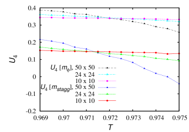
From the plots in Fig. 4, one sees that the critical temperature of the magnetic transition is $T_{AF}\simeq 0.9715\pm 0.0005$, while the critical temperature of the nematic transition is $T_{nem}\simeq 0.9720\pm 0.0005$. Therefore, within our accuracy, the two transitions occur at the same temperature.

To establish the universality class of the two transitions we apply the scaling analysis to the magnetic susceptibilities

$$\chi_{(\pi,0)}=\frac{\beta}{N}\left[\langle\sum_{i,j}\sigma_{i}\sigma_{j}\,{(-1)}^{(x_{j}-x_{i})}\rangle-{\langle\sum_{i}\sigma_{i}\,{(-1)}^{x_{i}}\rangle}^{2}\right];$$ (6a)

$$\chi_{(0,\pi)}=\frac{\beta}{N}\left[\langle\sum_{i,j}\sigma_{i}\sigma_{j}\,{(-1)}^{(y_{j}-y_{i})}\rangle-{\langle\sum_{i}\sigma_{i}\,{(-1)}^{y_{i}}\rangle}^{2}\right],$$ (6b)

and to the nematic susceptibility

$$\chi_{\phi}=\frac{\beta}{N}\left(\langle\sum_{i,j}\phi_{i}\phi_{j}\rangle-{\langle\sum_{i}\phi_{i}\rangle}^{2}\right).$$ (7)

We consider temperatures sufficiently close to the critical temperature, so that we can ignore the second term in the r.h.s. of the two equations, (i.e. the square of the order parameter). Indeed at the critical temperature this term vanishes like $t^{2\beta}$ (where $t=\left(T-T_{AF}\right)/T_{AF}$) and is negligible with respect to the correlation term (the first term in the r.h.s.) that tends to diverge like $t^{-\gamma}$.

We report the scaling function $\tilde{\chi}=L^{-\gamma/\nu}\chi(t)$ as a function of $L^{1/\nu}t$ for the three different system sizes. The susceptibilities for systems of different size must coincide if the critical exponents $\gamma$, $\nu$ and the critical temperature are exact and the transition is of the second order. In Fig.5 we show the scaling functions for the magnetic (we report only $\chi_{(0,\pi)}$) and nematic suscetibilities.

Figure 5: (Color online) $\chi_{(0,\pi)}$ and $\chi_{\phi}$ scaling functions for lattice size $10\times 10$ (triangles, red and magenta online), $24\times 24$ (circles, green and ligth blue), $50\times 50$ (squares, blue and black). The temperature step is $5\cdot 10^{-4}$. We have fixed $\gamma=7/6$, $\nu=2/3$, $T_{AF}=0.9715$ for the magnetic transition, and $\gamma=7.00/4.15$, $\nu=0.975$, $T_{nem}=0.9720$ for the nematic transition.

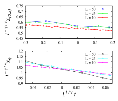
We find that a reasonable scaling is obtained with $\gamma=7/6$, $\nu=2/3$, $T_{AF}=0.9715$. These critical exponents correspond to a four-component Potts modelWu1982Potts . Indeed, the magnetic order of our system is described by the two parameters $m_{(\pi,0)}$ and $m_{(0,\pi)}$, each parameter having two possible values. Therefore the magnetic order parameter has 4 “colors” and threrefore one can naturally expect that the transition belongs to the four-component Potts model universality class. We remark that the transition is weakly first-orderLopez1993Firstorder and therefore the scaling found can only be approximate.

On the other hand it is natural to expect that the critical indexes of the nematic transition are those of the simple Ising modelHuang1987Statistical . We find $\gamma=7.00/4.15$, $\nu=0.975$, $T_{nem}=0.9720$, which are indeed rather close to the critical indexes of the twodimensional Ising model, but they do not quite coincide with them. Moreover the scaling functions of the three different system sizes do not collapse and are very close only when the reduced temperature $t$ is close to zero. Therefore the scaling found in this case is not ideal. This is not surprising given that this transition is also weakly first-order (see below). Moreover the two transitions occur simultaneously and can influence each other changing the universality class. In a more rigorous approach the Ising and the Potts order parameters would form a single order parameter with more components and a combined universality class. However the scaling found above shows that the decomposition in Ising and Potts is a good approximation.

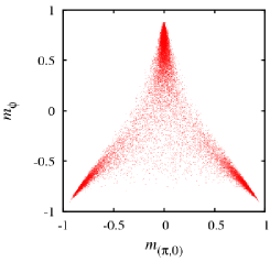
With the present choice of $R=0.60$ we find that there is no nematic phase. For example in Fig.6 we show the scatter plot for the system with size $L=50$ at the temperature $T=0.9720$, below which the nematic order parameter develops. There is no evidence of a nematic phase because there is no accumulation of points in the region with $m_{(\pi,0)}\simeq 0$ and $m_{\phi}<0$. Notice that the accumulation of points for $m_{\phi}>0$ corresponds to $(0,\pi)$ magnetic order. We find a qualitatively similar behavior at all intermediate temperatures up to the disordered temperature.

Figure 6: (Color online) Scatter plot in the 2D-spaces $\left[m_{(\pi,0)},m_{\phi}\right]$ resulting from the simulations of a $50\times 50$ lattice with $R=0.60$, at the temperature $T=0.9720$.

We now consider MC simulations for a $50\times 50$ system with $R=0.51$, that is very close to the critical point at $R=0.50$. This case has already been shown as an example in Fig.3. The panel (b) shows a coexistence of disorder and nematic order at $T=0.52$, because we see a maximum in the disordered region and a maximum in the nematic region ($[m_{(\pi,0)}\sim 0,\,m_{\phi}\neq 0]$. Making other histograms with higher level surfaces we see that the maximum of the disordered phase is lower than the one occurring in the nematic region. Therefore the disordered phase is metastable. The occurrence of two maxima in the phase space population, that is two minima in the free energy, also indicates that the transition from the disordered phase to the nematic phase is of the first-order. Fig.3(c) is a contour plot of the counts for each bin in the $[m_{(\pi,0)},m_{\phi}]$ 2D-space. In principle we should also study the $[m_{(0,\pi)},m_{\phi}]$ projection. However, since we made the two staggered magnetizations equivalent by exploiting the symmetries of the problem, we can focus on one of the two projections only.

Decreasing the temperature there is an increase of the counts (i.e., configurations) related to the magnetic phase, that is identified by finite values of $m_{(\pi,0)}$. The temperature at which these counts become higher than the ones at nematic region in the 3D representation, correspond to the critical temperature $T_{AF}$ of the nematic to magnetic transition. We show in Fig.7 the level curves of the bin counts in the $[m_{\pi,0},m_{\phi}]$ 2D-space, for a range of temperatures. Since also here there is coexistence of maxima in the nematic and the magnetic region the transition is first-order.

To compute the temperature range of the nematic phase we study the histograms of the simulations at different temperatures (we use $\Delta T=0.01$ steps in temperature).

Figure 7: (Color online) Level curves of the bin counts in the 2D-space $[m_{(\pi,0)},m_{\phi}]$ resulting from the simulations of a $50\times 50$ lattice, with $R=0.51$. Are shown the results for $T=0.53$, $T=0.52$, $T=0.51$, $T=0.50$. The higher is the brightness of the bins and the higher is the values of the counts.

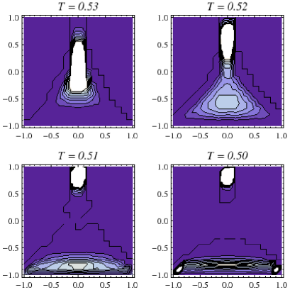
A close inspection of the level surfaces of the histograms in 3d-space [like the one shown in Fig.3(b)], we can state that at $T=0.53$ the maximum in correspondence to the disordered phase is higher than the one corresponding to the nematic phase. Similarly at $T=0.50$ the maximum of the smectic phase is the highest. Hence the range of temperatures in which the system has nematic order only includes the $T=0.51$ and $0.52$ temperatures.

Figure 8: (Color online) Magnetic configurations of a $50\times 50$ systems with $T=0.52$; (a) real spin configuration, where the red squares represent the spin-up, while the blue squares the spin-down, (b) staggered configuration along $y$ axis, where the squares are red if $\sigma_{i}\cdot{(-1)}^{y_{i}}=+1$, while they are blue if $\sigma_{i}\cdot{(-1)}^{y_{i}}=-1$.

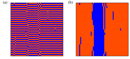
We show in Fig.8 the magnetic configuration at the end of the simulation at the temperature $T=0.52$. One can clearly see that rotational symmetry is broken, but the system does not display a complete magnetic order, because the average value of the staggered magnetization, which define the magnetic order is small. We also studied smaller systems with $24\times 24$ and $10\times 10$ lattice sites. Performing the same analysis as in the previous case, we observe that the range of temperatures where nematic order occurs is larger than in the $50\times 50$ system. We report in Fig.9 the same plots as in Fig.7 for the $24\times 24$ system at the two temperatures delimiting the nematic range.

Figure 9: (Color online) Level curves of the bin counts in the $[m_{(\pi,0)},m_{\phi}]$ 2D-space resulting from the simulations of a $24\times 24$ lattice, with $R=0.51$. The results for $T=0.54$ and $T=0.49$ are reported. The bins with highest counts are the most bright.

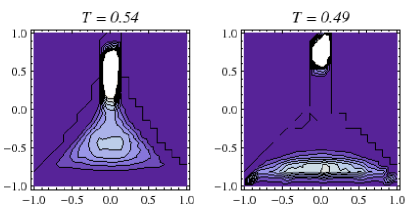
At the temperatures considered in Fig.9 there is still an evident nematic phase. For a $10\times 10$ lattice, the nematic range is even larger. We can therefore conclude that the smaller is the system size and the stronger is the tendency to form a nematic phase.

To explain this result we compute the energy cost to form a domain like the one displayed in Fig.2 on the perfect $(\pi,0)$ order. Notice that this corresponds to a change of phase of the magnetic order but without rotation of the direction of the stripes. These domains will be naturally elongated and we aim to find the typical aspect ratio.

We consider for simplicity a rectangular domain like the one shown in Fig.2. It is easy to see that the boundary energy is anisotropic. With respect to the ground state (complete smectic phase), a spin located along the vertical walls brings along an increase of energy per unit length of domain boundary $\Delta E_{ver}=2J_{1}+4J_{2}$. On the other hand, the increase of energy per unit length due to a spin located along the horizontal wall is given by $\Delta E_{hor}=-2J_{1}+4J_{2}$. We call $l_{\perp}$ the length of the walls perpendicular to the stripes, and $l_{\|}$ the length of the walls parallel to the stripe. The number of spins along the horizontal walls of the rectangular domain will be $2l_{\perp}$, while along the vertical walls they are $2l_{\|}$. Thus the boundary energy of the domain is given by

$$E_{bnd}=2l_{\perp}(-2J_{1}+4J_{2})+2l_{\|}(2J_{1}+4J_{2}).$$ (8)

We now determine what is the most stable configuration for this type of domains. To this purpose we minimize $E_{bnd}$ varying its aspect ratio $l_{\perp}/l_{\|}$, while maintaining its area $l_{\perp}l_{\|}$ fixed. We find,

$$\frac{l_{\perp}}{l_{\|}}=\frac{2J_{2}+J_{1}}{2J_{2}-J_{1}}=\frac{2R+1}{2R-1}.$$ (9)

Although this computation applies to the ordered phase, as the temperature is lowered from the disordered phase, we expect that elongated domains are formed with approximately the same aspect ratio. This defines two typical length scales $\xi_{\perp}$ and $\xi_{\|}$ corresponding to two different correlation lengths satisfying

$$\frac{\xi_{\perp}}{\xi_{\|}}=\frac{l_{\perp}}{l_{\|}}.$$ (10)

Approaching the Néel temperature $T_{AF}$ from above, the correlation lengths should be described by

$$\xi_{\perp}=\frac{\xi_{\perp}^{0}}{{|T-T_{AF}|}^{\nu}};$$ (11a)

$$\xi_{\|}=\frac{\xi_{\|}^{0}}{{|T-T_{AF}|}^{\nu}},$$ (11b)

where $\xi_{\perp}^{0}$ and $\xi_{\|}^{0}$ are simple proportionality factors, whose ratio is expected to be given by Eqs.(9) and (10).

For values of $R$ near $0.5$, we have $\xi_{\perp}^{0}\gg\xi_{\|}^{0}$ and there will be a range of temperatures for which the linear system size, $L$, satisfies

$$\xi_{\|}<L<\xi_{\perp}.$$ (12)

This means that the system is ordered in the direction perpendicular to the stripes but it is still disordered along the direction of the stripes. This is precisely the nematic phase. Indeed we can see in the snapshot of Fig. 8 (b) that the domains are elongated and span one linear dimension of the sample, while the system has a correlation smaller than $L$ in the direction parallel to the stripes.

As the system size increases the temperature range in which Eq. (12) is satisfied decreases, i.e. the nematic temperature window decreases with system size, in agreement with our simulations.

Simple arguments show that the value of $R$ in FeAs planes is actually close to its critical value $R=0.5$Dai . These results can also shed light on the experiments by Jesche et al.Jesche2010Coupling and Liang et al.. The former found that the splitting between the structural and the magnetic transition decreases as the sample quality is increased while the latter finds that the anisotropy in transport decreases. It is quite natural to assume that grain boundaries, dislocations and other defects will disrupt the perfect crystal order and introduce an extrinsic scale $L$ roughly given by the average distance among defects. As the sample is cooled from the disordered phase, at some point the longitudinal correlation length will exceed the scale $L$. Then at this scale $L$ the $C_{4}$ symmetry of the crystal will be spontaneously broken and the system will undergo a spontaneous orthorhombic distortion possibly with twining or domain formation at the scale $L$. In the perpendicular direction the system will remain essentially disordered preventing the appearance of an elastic signal in magnetic neutron scattering. At a lower temperature the system will become magnetically ordered in both directions.

This picture applies for weak magnetoelastic coupling. As we will show in the next Section, when the the spin system is strongly coupled to the lattice the structural and nematic transitions occur at the same temperature and the splitting between the structural and the magnetic transition coincides with the splitting between the nematic and the magnetic transition.

IV Spin-lattice coupling

In this Section we consider lattice deformations and their effects on the spin system. In the continuum the distortions can be characterized by the symmetric strain tensor

$$u_{\mu\nu}=\frac{1}{2}\left(\frac{\partial u_{\mu}}{\partial x_{\nu}}+\frac{\partial u_{\nu}}{\partial x_{\mu}}\right),$$ (13)

where $\mu$, $\nu$ label the Cartesian directions.

In a 2D system it is convenient to work with the following strains,

$$e_{1}=u_{xx}+u_{yy},\quad e_{2}=u_{xx}-u_{yy},\quad e_{3}=\sqrt{2}u_{xy},$$ (14)

which describe dilational, deviatoric and shear deformations respectively.

To include magnetoelastic effects in our frustrated Ising model, we assume that the coupling constant $J_{1i,\nu}$ among atom $i$ and the nearest-neighbour atom in the $\nu$ direction depends linearly on the deformation according to

$$J_{1i,x}=J_{1}+2\alpha u_{xx}=J_{1}+\alpha(e_{1}+e_{2}),$$ (15a)

$$J_{1i,y}=J_{1}+2\alpha u_{yy}=J_{1}+\alpha(e_{1}-e_{2}).$$ (15b)

For simplicity we will restrict to uniform strains which is enough to describe the observed structural transition. At lowest order the shear strain does not couple with the magnetism. The dilation strain $e_{1}$ simply adds to $J_{1}$ and describes symmetry preserving changes in the volume which are interesting but not the focus of the present work. Therefore we set $e_{1}=e_{3}=0$ and consider only $\epsilon\equiv e_{2}$. The latter is the order parameter of the observed structural transitionKrellner2008Magnetic ; delaCruz2008Magnetic which for a FeAs layers implies a deformation from a square lattice to a rectangular lattice. Within this approximation we obtain the magnetoelastic term

$$H_{M-el}=-\alpha\varepsilon\sum_{i=1}^{N}\sigma_{i}(\sigma_{i+x}-\sigma_{i+y})=-2\alpha\varepsilon\sum_{i=1}^{N}\phi_{i}.$$ (16)

In addition we must consider the elastic energy which is given by

$$H_{el}=\frac{1}{2}N\mu_{0}{\varepsilon}^{2},$$ (17)

where $\mu_{0}$ is a shear modulus at $T=0$.

We thus obtain a sum of three terms: the purely magnetic term Eq. (1), a purely elastic term Eq. (17) and the magnetoelastic term Eq. (16). This last term contributes to the internal energy $U\equiv\langle H\rangle$, by an amount $\langle H_{M-el}\rangle=-2N\alpha\varepsilon\langle m_{\phi}\rangle$, directly involving the thermal average of the nematic magnetization $\langle m_{\phi}\rangle$. Thus the nematic and structural order parameter couple linearly with each other. This implies that the nematic critical temperature should coincide with the critical temperature of the structural transition.

To identify the stable equilibrium states of the system at finite temperature, we now study the Helmholtz free energy. We start from values of temperature higher than both the critical temperature $T_{AF}$ of the magnetic transition and the critical temperature $T_{S}$ of the structural transition. Therefore no magnetic order and no structural deformations are present and the free energy will be minimum for $\langle m_{\phi}\rangle=0$ and $\varepsilon=0$. If we consider small variations of the two parameters $\langle m_{\phi}\rangle$ and $\varepsilon$ around their zero values, we can expand the free energy up to second order in the two variables thereby obtaining

$$\frac{\delta F(\langle m_{\phi}\rangle,\varepsilon)}{N}=\frac{1}{2}(\chi_{\phi}^{0})^{-1}{\langle m_{\phi}\rangle}^{2}+2\alpha\langle m_{\phi}\rangle\,\varepsilon+\frac{1}{2}\mu\,{\varepsilon}^{2},$$ (18)

Adding external fields coupling linearly with the order parameters one can see that $\chi_{\phi}^{0}$ is the same nematic susceptibility appearing in Eq. (7). The last coefficient $\mu$ is the shear modulus at finite temperature and in the absence of magnetoelastic coupling. Within our approximations we can consider this term equal to the coefficient $\mu_{0}$ of Eq.(17), since the elastic term (17) of the Hamiltonian coincides with the elastic free energy $F_{el}=\frac{1}{2}N\mu{\varepsilon}^{2}$. Indeed, since the deformation $\varepsilon$ is constant along the whole system, the lattice entropy is a quantity of order 1 and can safely be neglected when extensive quantities of order $N$ are considered. Minimizing Eq. (18) with respect to the nematic magnetization $\langle m_{\phi}\rangle$, we obtain

$$\langle m_{\phi}\rangle=-2\alpha\,\varepsilon\,\chi_{\phi}^{0}.$$ (19)

Replacing this expression of $\langle m_{\phi}\rangle$ into Eq.(18) we find

$$\delta F(\varepsilon)=\frac{1}{2}N\left(\mu_{0}-4\alpha^{2}\chi_{\phi}^{0}\right)\,{\varepsilon}^{2}=\frac{1}{2}N\,\mu_{tot}\,{\varepsilon}^{2},$$ (20)

where $\mu_{tot}(T)$ is the temperature dependent shear modulus, which takes into account the renormalization due to magnetoelastic coupling.

Introducing an effective coupling constant $\lambda=4\alpha^{2}/\mu_{0}$, from Eq. (20) one obtains a generalized Stoner criterium. If $\chi_{\phi}^{0}(T)<1/\lambda$, the system is stable, whereas, if $\chi_{\phi}^{0}(T)>1/\lambda$, the system becomes unstable and gains energy by making a deformation $\varepsilon$. The temperature at which $\chi_{\phi}^{0}(T)=1/\lambda$ defines the critical temperature $T_{S}^{2nd}$ of the (second-order) structural transition.

Let’s assume that in the absence of magnetoelastic coupling, the transitions are second order and that the nematic and magnetic susceptibility diverge at the same temperature, i.e. that there is no true thermodynamic nematic phase for $\alpha=0$. The above argument shows that for small magnetoelastic coupling the nematic and the orthorhombic orders occur simultaneously at the temperature $T_{S}^{2nd}$ higher than that of magnetic order. Indeed in the disordered phase, the nematic susceptibility $\chi_{\phi}^{0}$ will grow upon lowering the temperature and the instability (Stoner-like) condition will be satisfied while the magnetic susceptibility is still finite. Although the presence of the structural distortion will tend to increase the Neel temperature $T_{AF}$, this increased temperature can never reach $T_{S}^{2nd}$ since $\epsilon$ vanishes at $T_{S}^{2nd}$. Therefore a finite temperature window should appear between $T_{S}^{2nd}$ and $T_{AF}$. Thus the magnetoelastic coupling can induce a nematic phase. Of course, if the nematic phase were already existing for $\alpha=0$, a small magnetoelastic coupling would tend to widen the nematic temperature window.

Notice that the above arguments are general and do not depend on the details of the model (e.g. Ising vs. Heisenberg) but on the second order character of the transition. We will show below that the weakly first-order character is enough to change this scenario. For a first order transition occurring at $T_{S}^{1st}$ the temperature $T_{S}^{2nd}$ where the shear modulus vanishes satisfy $T_{S}^{2nd}<T_{S}^{1st}$ and corresponds to the limit of stability of the metastable disordered phase.

In order to investigate the feedback effect of the lattice on the magnetic transition and the effect of the first-order character we carry out a Monte Carlo study of the magnetoelastically coupled Hamiltonian. To take into account the thermal fluctuation of the deformation parameter $\Delta J=\alpha\varepsilon$, every $n$ Monte Carlo step (where $n$ is the number of the lattice sites) we allow for random variations of this parameter in a certain range (we use $[-0.2:0.2]$). Each variation of $\Delta J$ is accepted or refused according to Metropolis algorithm with the energy given by Eqs.(1), (16) and (17). We perform temperature runs (with a step $\Delta T=0.01$) of a $50\times 50$ system with $R=0.51$, for several values of $\lambda$.

The phase diagram in the $[\lambda,T]$ space, resulting from our simulations, is reported in Fig.10.

Figure 10: (Color online) Phase diagram of the system with $R=0.51$ in the $\lambda$ vs. $T]$ space. We report the numerical results for the structural (or nematic) critical temperatures (open circles, blue online) and the magnetic critical temperatures (open squares, green online), and the structural critical temperatures in the stability limit (open circles, red online, joined by the solid line). The shaded (magenta online) region represents the nematic range in a $50\times 50$ lattice. The inset displays an expansion of the nematic region of the phase diagram. The nematic range in a $24\times 24$ system (darker shaded region, yellow online) is also shown.

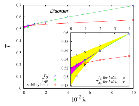
We see that increasing $\lambda$, the temperature interval with nematic order shrinks and it disappears completely for $\lambda=2.0\cdot 10^{-2}$. Thus the largest nematic window is for $\lambda=0$ and it correspond to the case studied in the previous section. This goes against our original expectation to find an enhanced nematic phase in the presence of the magnetoelastic coupling. Such a failure is clearly due to the first order character of the transition which gets enhanced by the magnetoelastic coupling. This can be recognized from the fact that $T_{S}^{2nd}$ and $T_{S}^{1st}$ practically coincide for $\lambda=0$, while $T_{S}^{1st}$ becomes substantially larger than $T_{S}^{2nd}$ as $\lambda$ increases. This is also supported by the presence of thermal hysteresis of the order parameters that we observe at high values of $\lambda$.

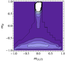
Notice that as expected $T_{S}^{2nd}$ increases with $\lambda$ but $T_{AF}$ increases more and due to the first-order character of the structural transition this renormalization of $T_{AF}$ can reach $T_{S}^{1st}$ closing the nematic window. As discussed in the previous Section, this window is larger for smaller system sizes. Indeed, as it is shown in the inset of Fig.10), in a $24\times 24$ system a larger nematic region in the $[\lambda,T]$ space is found. Although increasing $\lambda$ leads to the closing of the nematic window, a nematic phase does exist at small spin-lattice coupling: We report in Fig.11 a contour plot of the order parameter distribution function for $\lambda=1.0\cdot 10^{-2}$ which shows clearly that the system is in a nematic phase.

Figure 11: (Color online) Contour plot of the order parameter distribution projected in the $[m_{(\pi,0)},m_{\phi}]$ plane resulting from the simulations of a $50\times 50$ lattice, with $R=0.51$ and $\lambda=1.0\cdot 10^{-2}$, at $T=0.538$.

In short we can state that for small $\lambda$, transitions from disordered phase to nematic phase and from nematic phase to magnetic phase are both only ‘weakly’ of the first-order. Therefore our schematic model system grossly reproduces the features of the 1111 delaCruz2008Magnetic or of Ba(Fe_1-xCo_x)₂As₂ fernandes1 ; nandi materials, where a separation between a second-order structural transition and a second-order magnetic transition is observed. In particular we notice that, upon increasing doping in Ba(Fe_1-xCo_x)₂As₂ the nematic window increases becoming largest at $x\gtrsim 0.06$, near optimal doping nandi . This strengthening of the nematic state finds a rational within our findings because increasing doping naturally leads to a decrease of magnetoelastic couping $\lambda$ and to an increase of disorder. As found in our schematic model, both these effects increase the nematic region between the structural and the magnetic transitions (cf. the inset of Fig. 10). We also notice that estimates from shear modulus measurements in Ba(Fe_1-xCo_x)₂As₂ give typical values of $\lambda\lesssim 5\cdot 10^{-3}$, substantially smaller than the values at which the nematic windows closes in our Fig. 10).

When instead we choose a high value of $\lambda$, we obtain a system which grossly reproduces the behavior of many 122 materialsKrellner2008Magnetic where the structural and magnetic transitions are strongly first-order and occur at the same temperature. We furthermore notice that when the transitions become strongly of the first-order, the value of the critical temperature increases. Although the precise value of the critical temperature will depend on many other parameters it is interesting that the critical temperature of the ‘122’ materials are substantially higher than the critical temperatures of the ‘1111’ materials.

V Conclusions

In this paper we investigated numerically and with simple analytic arguments the possible occurrence of a nematic phase and the associated splitting of the structural and magnetic transitions in FeAs planes. We analyzed a schematic model of Ising spins with nearest and next-nearest neighbor couplings. The effects of a spin-lattice coupling has also been considered. First of all we find that for $R$ larger than (but close to) 1/2 the model displays a weakly first-order transition. The very weak first-order character found in the absence of lattice coupling allows to study critical exponents which for the magnetic order parameter, are close to the ones of a 4-state Potts model in agreement with simple symmetry considerations.

One can then remark that the magnetic Potts order parameter can order at finite temperature even in two dimensions and therefore long range magnetic order effectively competes with the Ising nematic order. This model, therefore, has the double advantage of being more easily solved in numerical MC approaches and of being an “acid” test for the occurrence of nematic order. In addition, as we argue in the introduction, collective magnetism produces a system with large connectivity of the magnetic Hamiltonian, which makes the thermal transition rather mean-field like. We argue that such mean-field transition in a real lattice with 3D couplings and weak anisotropies is more similar to a 2D Ising transition than to a 2D Heisenberg transition. Thus, despite the apparent obvious difference in symmetry between our model and a real system, the model for some aspects is expected to be more realistic than a frustrated 2D Heisenberg model.

Our numerical study indicates that in the region of the stripe ground state, but close to the transition to the Néel AF phase ($R\gtrsim 0.5$), nematic states can form due to finite size effects in some temperature range above the magnetic order (the smaller is the length scale and the larger is the temperature range). We argue that such finite size effects are a proxy for the effect of crystal imperfections which disrupt the perfect lattice order and provide a natural explanation for the results of Jesche et al.Jesche2010Coupling and Liang et al.liang who find more robust nematic signatures in the worst quality samples.

The increase in resistivity anisotropyliang with decreasing sample quality has also been explained by Fernandes et al.fernandes2 in terms of the interplay between scattering of carriers by spin fluctuations and disorder.fernandes2 We believe both Ref. fernandes2, mechanism and the present one can contribute to the observed effect. More experimental and theoretical work would be needed to determine which one will be dominant in the different regimes.

We have neglected all Heisenberg physics which is expected to enhance the tendency to nematic phases.larkin ; Fang2008Theory However our arguments for the enhancement of the nematic phase in imperfect systems also applies to other models. For example also in a more realistic 3D Heisenberg model, possibly with long range couplings and anisotropies, the domains will be elongated and there will be two characteristic length scales, so that our arguments remain valid.

It is sometimes argued that, since the structural transition occurs at a higher temperature than the magnetic transition, it is the structure that drives the magnetism. This argument is clearly wrong and our model is another counterexample which show that the structural transition can occur at a higher temperature than the magnetism although it is driven by the magnetism itself. This is because the structural transition is driven by the cohesive energy which is determined by short range correlations like $\langle\sigma_{i}\sigma_{j}\rangle$ with $i$ and $j$ close neighbors. Thus cooling the system one can have a robust short range $\langle\sigma_{i}\sigma_{j}\rangle$, which renders the lattice unstable, before the system has long range magnetic order. Formalizing this argument in the case of second order transitions, one obtains the additional result that the coupling to the lattice favors the nematic state. However in the simulations we find the opposite because the lattice tends to make the transition more first-order like. This suggest that the nematic state observed is mainly driven by the electronic degrees of freedom and that the lattice act as a spectator, as suggested in Ref. Fang2008Theory, .

The different behavior found for weak and strong magnetoelastic coupling corresponds well with the behavior found on different pnictide families. Indeed 122 materials have larger critical temperature, first-order transitions a non-nematic state, as found for strong magnetoelastic coupling. On the other hand 1111 systems have lower transition temperatures, second-order or weakly first-order transitions and a nematic state as found for weak magnetoelastic coupling.