Towards designing robust coupled networks

Abstract

Natural and technological interdependent systems have been shown to be highly vulnerable due to cascading failures and an abrupt collapse of global connectivity under initial failure. Mitigating the risk by partial disconnection endangers their functionality. Here we propose a systematic strategy of selecting a minimum number of autonomous nodes that guarantee a smooth transition in robustness. Our method which is based on betweenness is tested on various examples including the famous $2003$ electrical blackout of Italy. We show that, with this strategy, the necessary number of autonomous nodes can be reduced by a factor of five compared to a random choice. We also find that the transition to abrupt collapse follows tricritical scaling characterized by a set of exponents which is independent on the protection strategy.

Interconnected complex networks are ubiquitous in today’s world. They control infrastructures of modern society (energy-communication-transportation), the financial system or even the human body Peerenboom01 ; Rosato08 ; Schweitzer09 . Unfortunately, they are much more fragile than uncoupled networks as recently recognized through the finding that the robustness changes from a second order transition in uncoupled systems to first order in interdependent systems Buldyrev10 ; Brummitt12 ; Gao2012 . The obvious mitigation strategy consists in partially decoupling the networks by the creation of autonomous nodes Parshani10 . Too much disconnection however risks endangering the functionality of the system. The question which we will address here is how to reduce fragility without losing functionality and we will in fact answer this question by developing an explicit algorithm based on betweenness that enables to avoid the abrupt collapse with a minimum number of autonomous nodes.

Figure 1: The herein proposed strategy improves significantly the resilience of the coupling between the communication system (39 stars) and the power grid (310 circles) in Italy. The color scheme stands for the probability that the node is inactive after the random failure of $14$ communication servers. In a) all communication servers are coupled while in b) four servers have been decoupled following the strategy proposed here. The coupling between the networks was established based on the geographical location of the nodes, such that each communication server is coupled with the closest power station Rosato08 . The images were produced using the software Pajek.

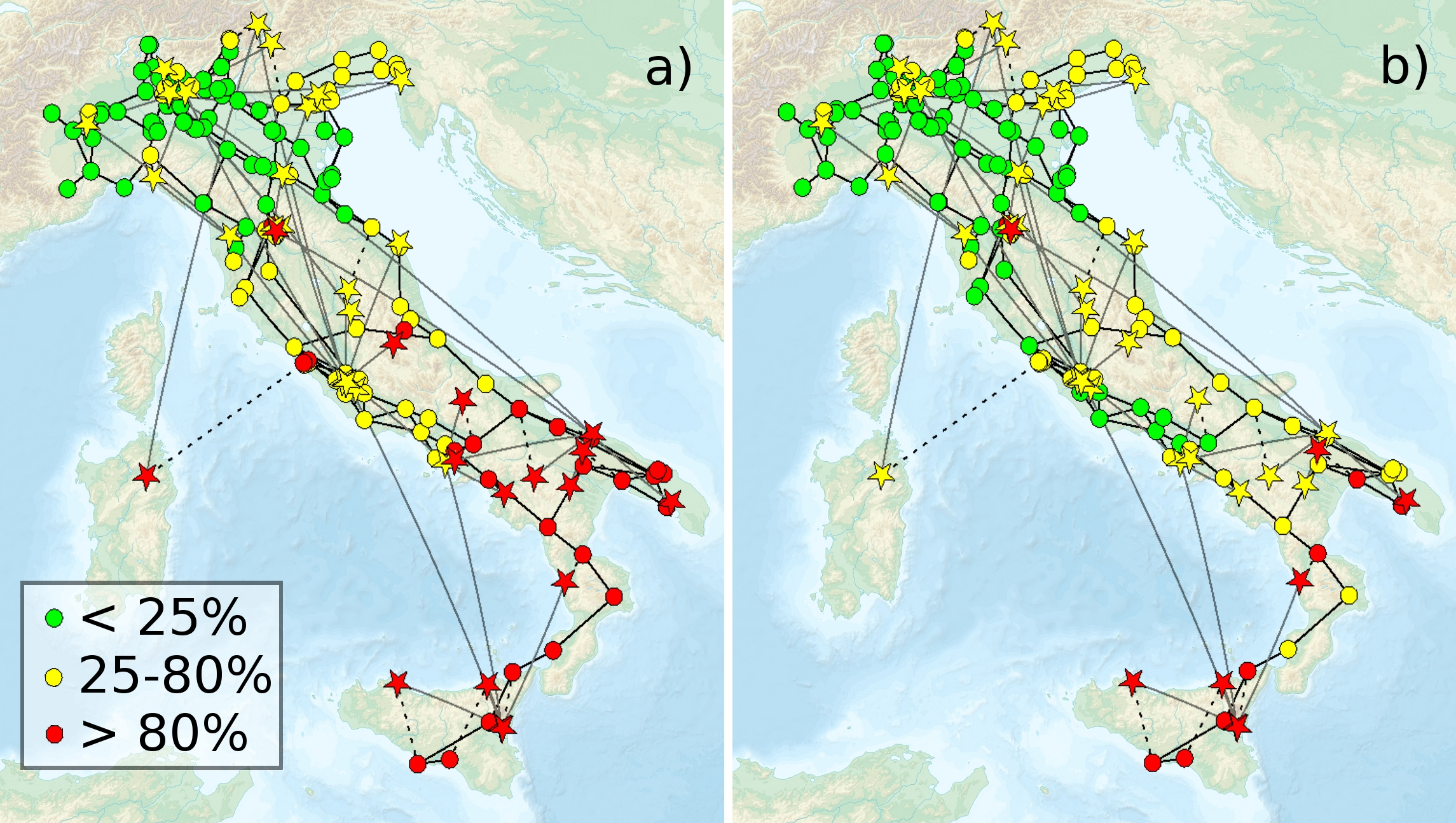
Buldyrev et al. Buldyrev10 proposed a percolation framework to study two coupled networks, $A$ and $B$, where each $A$-node is coupled to a $B$-node, via bi-directional links, such that when one fails the other cannot function either. The removal of a fraction of $A$-nodes may trigger a domino effect where, not only their counterparts in $B$ fail, but all nodes that become disconnected from the giant cluster of both networks also fail. This causes further cascading of failures, yielding an abrupt collapse of connectivity, characterized by a discontinuous (first order) percolation transition. Parshani et al. Parshani10 showed that damage can be mitigated by decreasing the degree of coupling, but only if a significant fraction ($\approx 0.4$) of nodes is decoupled, the transition changes from discontinuous to continuous. The coupling is reduced by randomly selecting a fraction of nodes to become autonomous and, therefore, independent on the other network. For the coupling between power stations and communication servers, for example, autonomous power stations have alternative communication systems which are used when the server fails and an autonomous server has its own energy power supply. We propose a method, based on degree and centrality, to identify these autonomous nodes that maximize the robustness of the system in terms of connectivity. We show that, with this scheme, the critical coupling increases, i.e., the fraction of nodes that needs to be decoupled to smoothen out the transition is much smaller (close to $0.1$ compared to $0.4$). Significant improvement is observed for different coupled networks including for Erdős-Rényi graphs (ER) where such improvement in the robustness was unexpected given their narrow degree distribution. To demonstrate the strength of our approach, in Fig. 1 we apply the proposed strategy to the real coupled system in Italy Rosato08 and show that by only protecting four servers the robustness is significantly improved (details in the figure caption).

Figure 2: Scheme of the cascade of node failures triggered by the initial failure of a node in network $A$ (top network). Two networks, $A$ (top) and $B$ (bottom), are considered. When a node initially fails in network $A$ (a) all nodes connected to the largest component through it also fail (b) as well as the corresponding dependent nodes in network $B$ (c). The failure of the dependent nodes in network $B$ leads to further failures in both networks (d) and (e). For each iteration step, the degree of coupling $q_{x}$ and the size of the largest connected component $S_{x}$ for each network $x$ are listed in (f).

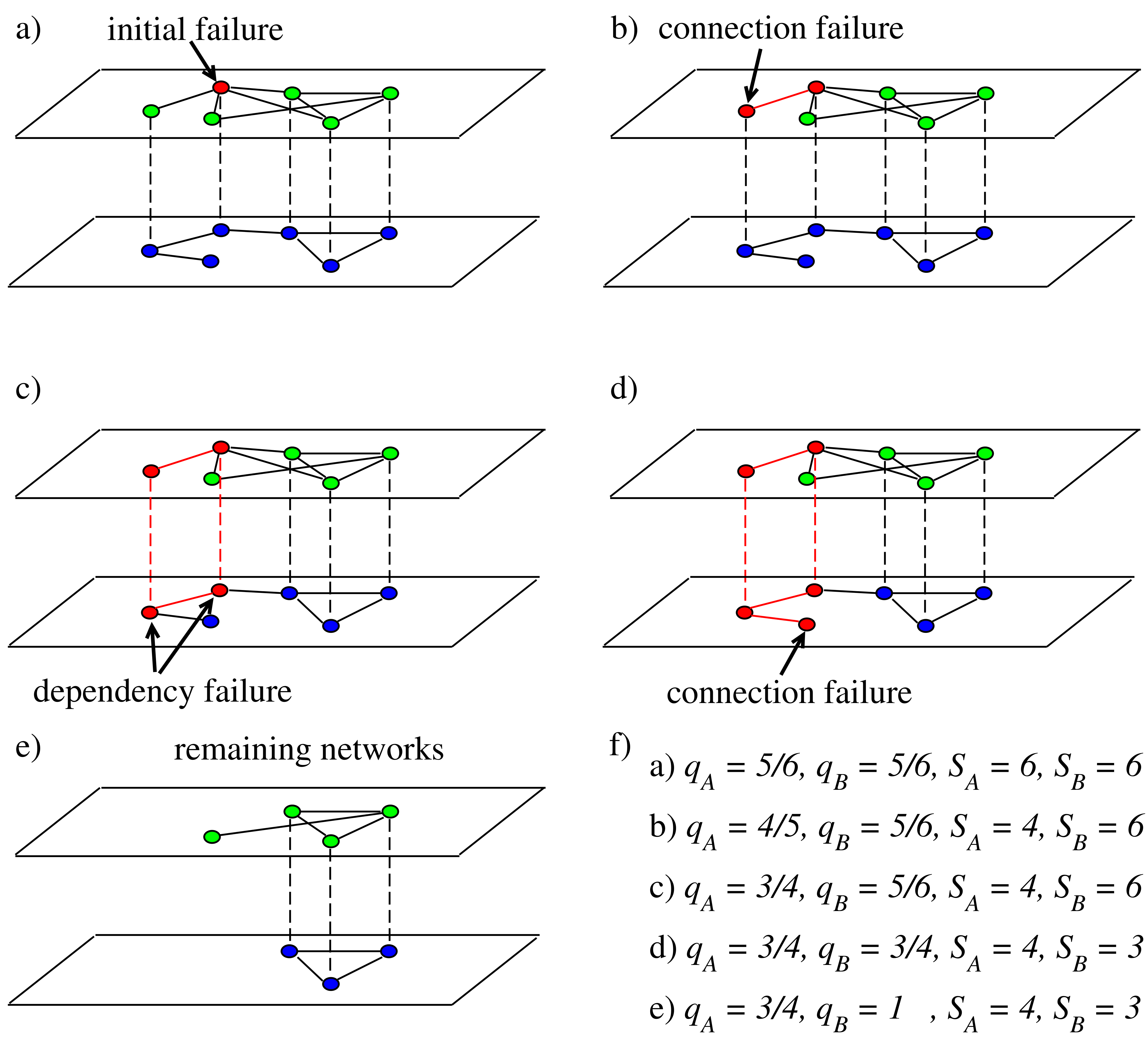
We consider a pair of networks, $A$ and $B$, where a fraction $q$ (degree of coupling) of $A$-nodes are coupled with $B$-nodes. To be functional, nodes need to be connected to the giant cluster of their network. When an $A$-node fails, the corresponding one in $B$ cannot function either. Consequently, all nodes bridged to the largest cluster through these nodes, together with their counterpart in the other network, become also deactivated. A cascade of failures occurs with drastic effects on the global connectivity (see Fig. 2) Buldyrev10 ; Parshani10 . This process can also be treated as an epidemic spreading Son11b . To study the resilience to failures, we follow the size of the largest connected cluster of active $A$-nodes, under a sequence of random irreversible attacks to network $A$. Notwithstanding the simplicity of solely considering random attacks, this model can be straightforwardly extended to targeted ones Huang10 . Recently, for single networks, it has been proposed Schneider11 to quantify the robustness $R$ as

$$R=\frac{1}{N}\sum_{Q=1}^{N}S(Q)\ \ ,$$ (1)

where $Q$ is the number of node failures, $S(Q)$ the size of the largest connected cluster in a network after $Q$ failures, and $N$ is the total number of nodes in the network Schneider11 ; Herrmann10 . Here we extend this definition to coupled systems by performing the same measurement, given by Eq. (1), only on the network where the random failures occur, namely, network $A$. To follow the cascade triggered by the failure of a fraction $1-p$ of $A$-nodes, similar to Parshani10 , we solve the iterative equations,

$$\beta_{n} = 1-q_{\beta,n}\left[1-S_{A}\left(\alpha_{n}\right)p\right],$$ (2)

$$\alpha_{n} = p\left(1-q_{\alpha,n}\left[1-S_{B}\left(\beta_{n-1}\right)\right]\right),$$ (3)

with the initial condition $\alpha_{1}=p$, where $\alpha_{n}$ and $\beta_{n}$ are the fraction of $A$ and $B$ surviving nodes at iteration step $n$ and $S_{x}(\chi_{n})$ is the fraction of such nodes in the giant cluster. $q_{\chi,n}$ is the fraction of dependent nodes in network $\chi$ fragmented from the largest cluster (see Methods for further details).

Results

Figure 3: Fraction of $A$-nodes in the largest connected cluster, $s$, as a function of the fraction of randomly removed nodes $1-p$ from network A, for two coupled ER (average degree $\langle k\rangle=4$) with $90\%$ of the nodes connected by inter-network links ($q=0.9$). It is seen that robustness can significantly be improved by properly selecting the autonomous nodes. We start with two fully interconnected ER and decouple $10\%$ of their nodes according to three strategies: randomly ((black-)solid line), the ones with highest degree in network $A$ ((red-)dotted line) and in network $B$ ((blue-)dashed line). We also include the case where $10\%$ autonomous nodes in both networks are chosen as the ones with highest degree and all the others are interconnected randomly ((green-)dotted-dashed line). The inset shows the dependence of the relative robustness of the degree strategy on the degree of coupling $q$ compared with the random case. Results for the degree have been obtained with the formalism of generation functions (see Methods).

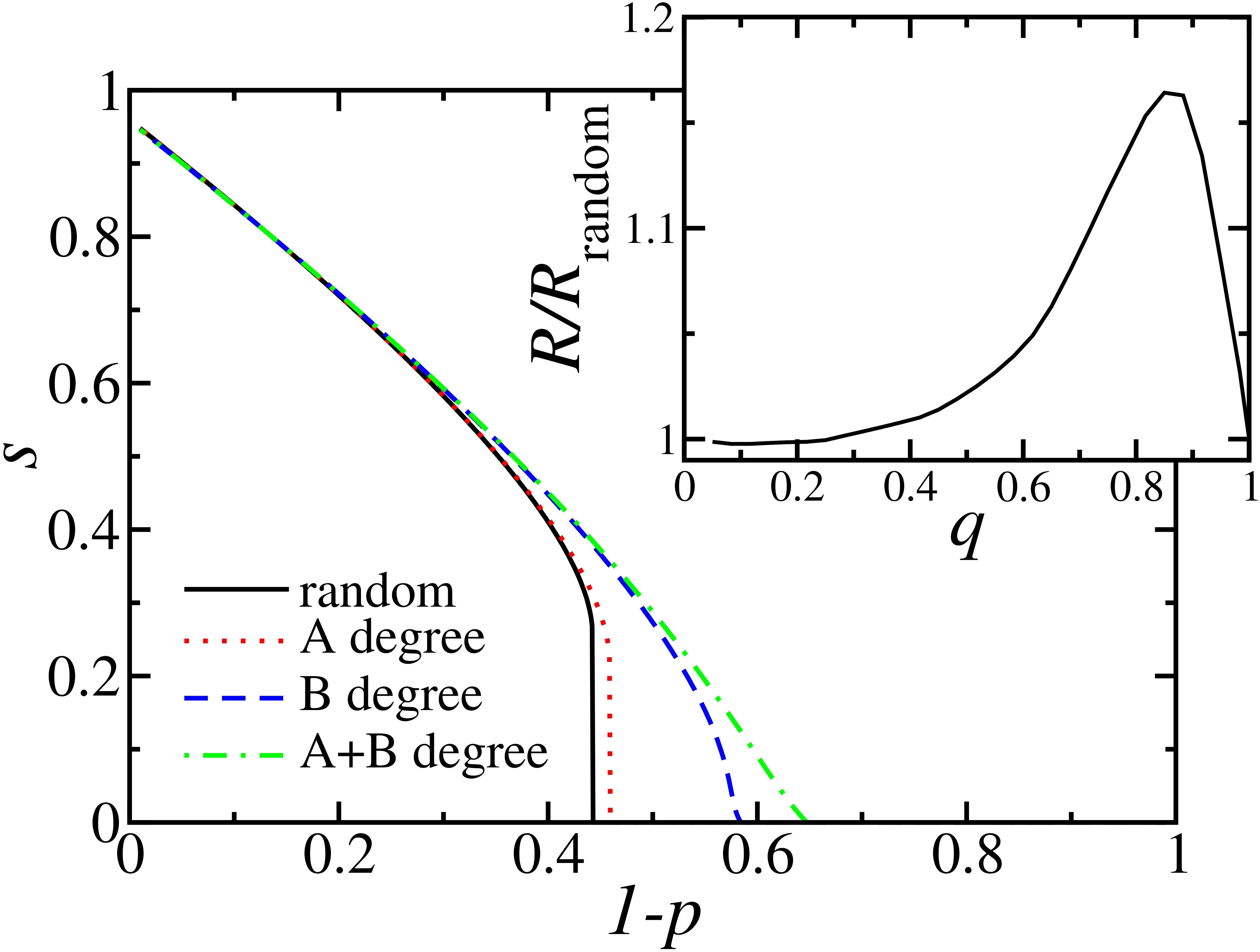
To demonstrate our method of selecting autonomous nodes we consider two ER graphs with average degree $\langle k\rangle=4$ and $10\%$ of autonomous nodes ($q=0.1$). First we consider a method based on the degree of the node and later we compare with the method based on the betweenness. Under a sequence of random failures, the networks are catastrophically fragmented when close to $45\%$ of the nodes fail, as seen in Fig. 3. For a single ER, with the same average degree, the global connectivity is only lost after the failure of $75\%$ of the nodes. Figure 3 also shows ((green-)dotted-dashed line) the results for choosing as autonomous nodes in both networks the fraction $1-q$ of the nodes with the highest degree and coupling the remaining ones at random. With this strategy, the robustness $R$ can be improved and the corresponding increase of $p_{c}$ is about $40\%$, from close to $0.45$ to close to $0.65$. Also the order of the transition changes from first to second order. Further improvement can be achieved if additionally the coupled nodes are paired according to their position in the ranking of degree, since interconnecting similar nodes increases the global robustness Parshani10c ; Buldyrev11 . In the inset of Fig. 3 we see the dependence on $q$ of the relative robustness for the degree strategy compared to the random case $R/R_{\mathrm{random}}$. For the entire range of $q$ the proposed strategy is more efficient and a relative improvement of more than $15\%$ is observed when still $85\%$ of the nodes are coupled.

Two types of technological challenges are at hand: either a system has to be designed robust from scratch or it already exists, constrained to a certain topology, but requires improved robustness. In the former case, the best procedure is to choose as autonomous the nodes with highest degree in each network and couple the others based on their rank of degree. For the latter, rewiring is usually a time-consuming and expensive process, and the creation of new autonomous nodes may be economically more feasible. The simplest procedure consists in choosing as autonomous both nodes connected by the same inter-network link. However, a high degree node in network $A$ is not necessarily connected with a high degree node in network $B$. In Fig. 3 we compare between choosing the autonomous pairs based on the degree of the node in network $A$ or in network $B$. When pairs of nodes are picked based on their rank in the network under the initial failure (network $A$), the robustness almost does not improve compared to choosing randomly. If, on the other hand, network $B$ is considered, the robustness is significantly improved, revealing that this scheme is more efficient. This asymmetry between $A$ and $B$ network is due to the fact that we attack only nodes in network $A$, triggering the cascade, that initially shuts down the corresponding $B$-node. The degree of this $B$-node is related to the number of nodes which become disconnected from the main cluster and consequently affect back the network $A$. Therefore, the control of the degree of vulnerable $B$-nodes is a key mechanism to downsize the cascade. On the other hand, when a hub is protected in network $A$ it can still be attacked since the initial attack does not distinguish between autonomous and non-autonomous nodes.

Figure 4: Dependence of the robustness, $R$, on the degree of coupling, $q$, for two, interconnected, (a) ER (average degree $\langle k\rangle=4$) and (b) SF with degree exponent $\gamma=2.5$. Applying our proposed strategy is applied, the optimal fraction of autonomous nodes is relatively very small. Autonomous nodes are chosen in four different ways: randomly ((blue-)triangles), high degree ((black-)dots), high betweenness ((red-)stars), and high k-shell ((yellow-)rhombi). The insets show the relative improvement of the robustness, for the different strategies of autonomous selection compared with the random case. Results have been averaged over $10^{2}$ configurations of two networks with $10^{3}$ nodes each. For each configuration we averaged over $10^{3}$ sequences of random attacks.

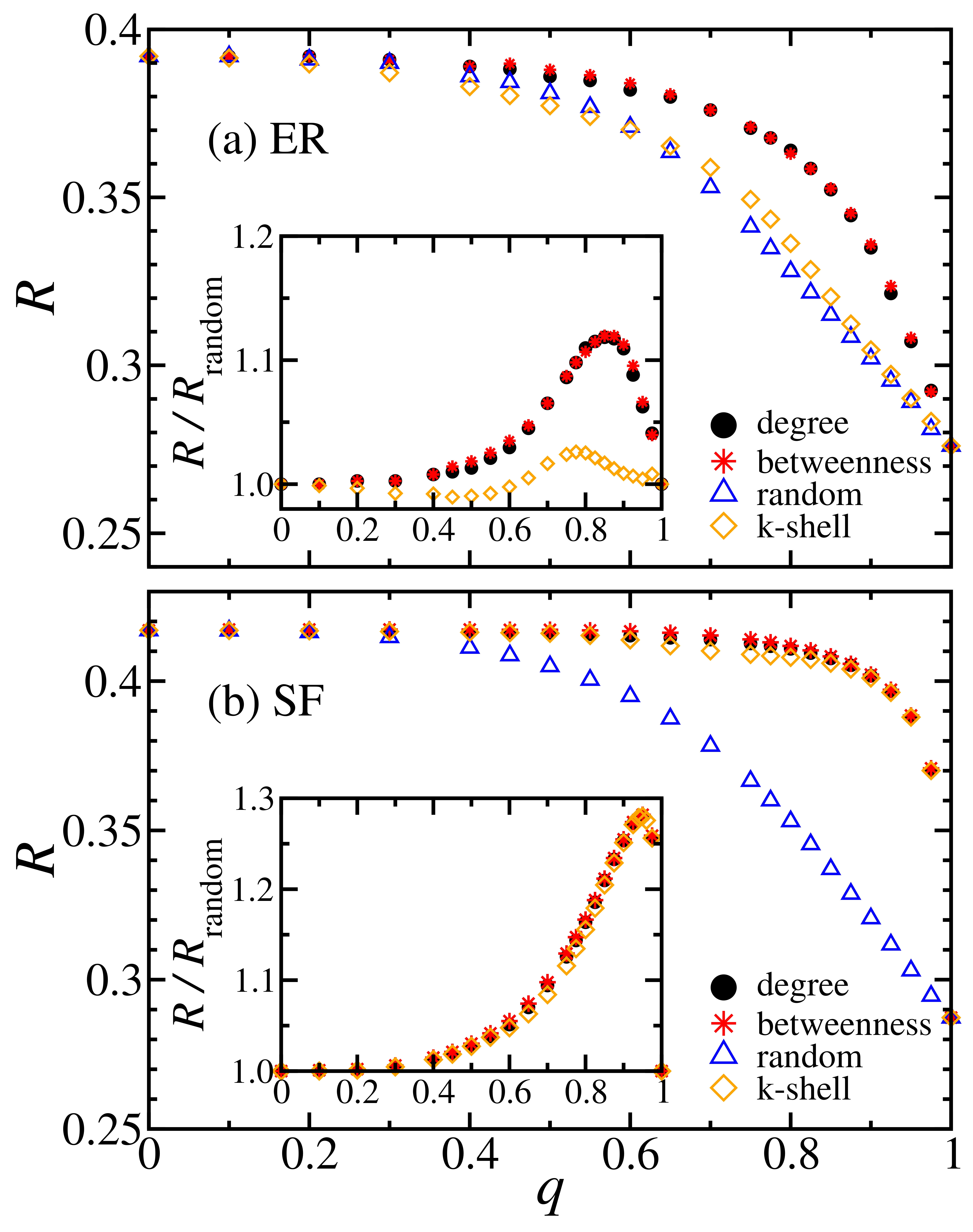
In Fig. 4(a) we compare four different criteria to select the autonomous nodes: betweenness, degree, k-shell, and random choice, for two coupled ER networks. In the betweenness strategy, the selected autonomous are the ones with highest betweenness. The betweenness is defined as the number of shortest paths between all pairs of nodes passing through the node Newman10 . A k-shell is obtained by removing, iteratively, all nodes with degree smaller than $k$, until all remaining nodes have degree $k$ or larger. In the k-shell strategy, the autonomous are chosen as the ones with highest k-shell in the k-shell decomposition Carmi07 . The coupled nodes (not autonomous), for all cases, have been randomly inter-linked. Since ER networks are characterized by a small number of k-shells, this strategy is even less efficient than the random strategy for some values of $q$, while the improved robustness for degree and betweenness strategies is evident compared with the random selection. While in the random case, for $q\gtrsim 0.4$, a significant decrease of the robustness with $q$ is observed, in the degree and betweenness cases, the change is smoother and only significantly drops for higher values of $q$. A maximum in the ratio $R/R_{\mathrm{random}}$ occurs for $q\approx 0.85$, where the relative improvement is above $12\%$. Since, in random networks, many metrics are strongly correlated Newman10 , the results for betweenness and degree are similar.

Many real-world systems are characterized by a degree distribution which is scale free with a degree exponent $\gamma$ Albert00 ; Clauset09 . In Fig. 4(b) we plot $R$ as a function of $q$ for two coupled scale-free networks (SF) with $10^{3}$ nodes each and $\gamma=2.5$. Similar to the two coupled ER, this system is also significantly more resilient when the autonomous nodes are selected according to the highest degree or betweenness. For values of $q\lesssim 0.85$ the robustness is similar to that of a single network ($q=0$) since the most relevant nodes are decoupled. A peak in the relative robustness, $R/R_{\mathrm{random}}$ (see inset of Fig. 4b), occurs for $q\approx 0.95$ where the improvement, compared to the random case, is almost $30\%$. Betweenness, degree, and $k$-shell, have similar impact on the robustness since these three properties are strongly correlated for SF. From Fig. 4, we see that, for both SF and ER, the robustness is significantly improved by decoupling, based on the betweenness, less than $15\%$ of the nodes. Studying the dependence of the robustness on the average degree of the nodes we conclude that for average degree larger than five, even $5\%$ autonomous nodes are enough to achieve more than $50\%$ of the maximum possible improvement.

Figure 5: Dependence of the robustness, $R$, on the degree of coupling, $q$, for two, randomly interconnected modular networks with $2\cdot 10^{3}$ nodes each. The modular networks were obtained from four Erdős-Rényi networks, with $500$ nodes each and average degree five, by randomly connecting each pair of modules with an additional link. Autonomous nodes are selected in three different ways: randomly (blue triangles), higher degree (black dots), and higher betweenness (red stars). In the inset we see the relative enhancement of the robustness, for the second and third schemes of autonomous selection compared with the random case. Results have been averaged over $10^{2}$ configurations and $10^{3}$ sequences of random attacks to each one.

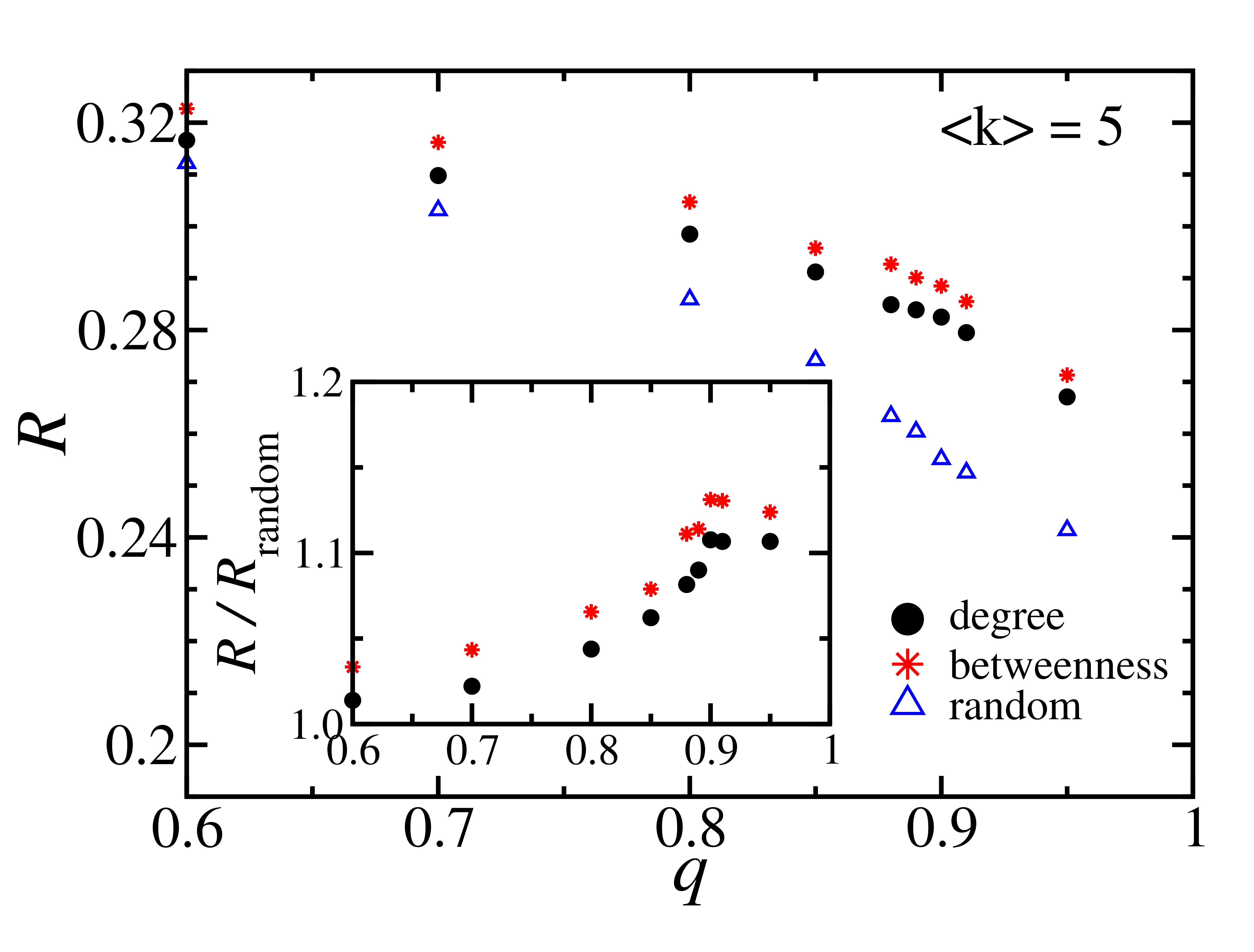
For the cases discussed in Fig. 4, results obtained by selecting autonomous nodes based on the highest degree do not significantly differ from the ones based on the highest betweenness. This is due to the well known finding that for Erdős-Rényi and scale-free networks, the degree of a node is strongly correlated with its betweenness Newman10 . However, many real networks are modular, i.e., composed of several different modules interconnected by less links, and then nodes with higher betweenness are not, necessarily, the ones with the largest degree Cohen10 . Modularity can be found, for example, in metabolic systems, neural networks, social networks, or infrastructures Ravasz02 ; Happel94 ; Gonzalez07 ; Eriksen03 . In Fig. 5 we plot the robustness for two coupled modular networks. Each modular network was generated from a set of four Erdős-Rényi networks, of $500$ nodes each and average degree five, where an additional link was randomly included between each pair of modules. For a modular network, the nodes with higher betweenness are not necessarily the high-degree nodes but the ones bridging the different modules. Figure 5 shows that the strategy based on the betweenness emerges as better compared to the high degree method.

Figure 6: Dependence of the robustness, $R$, on the degree of coupling, $q$, for two, randomly interconnected random regular graphs with $8\cdot 10^{3}$ nodes each, all with degree four. Autonomous nodes are selected in two different ways: randomly (blue triangles) and higher betweenness (red stars). In the inset the relative enhancement of the robustness is shown for the betweenness compared to the random case. Results have been averaged over $10^{2}$ configurations and $10^{3}$ sequences of random attacks to each one.

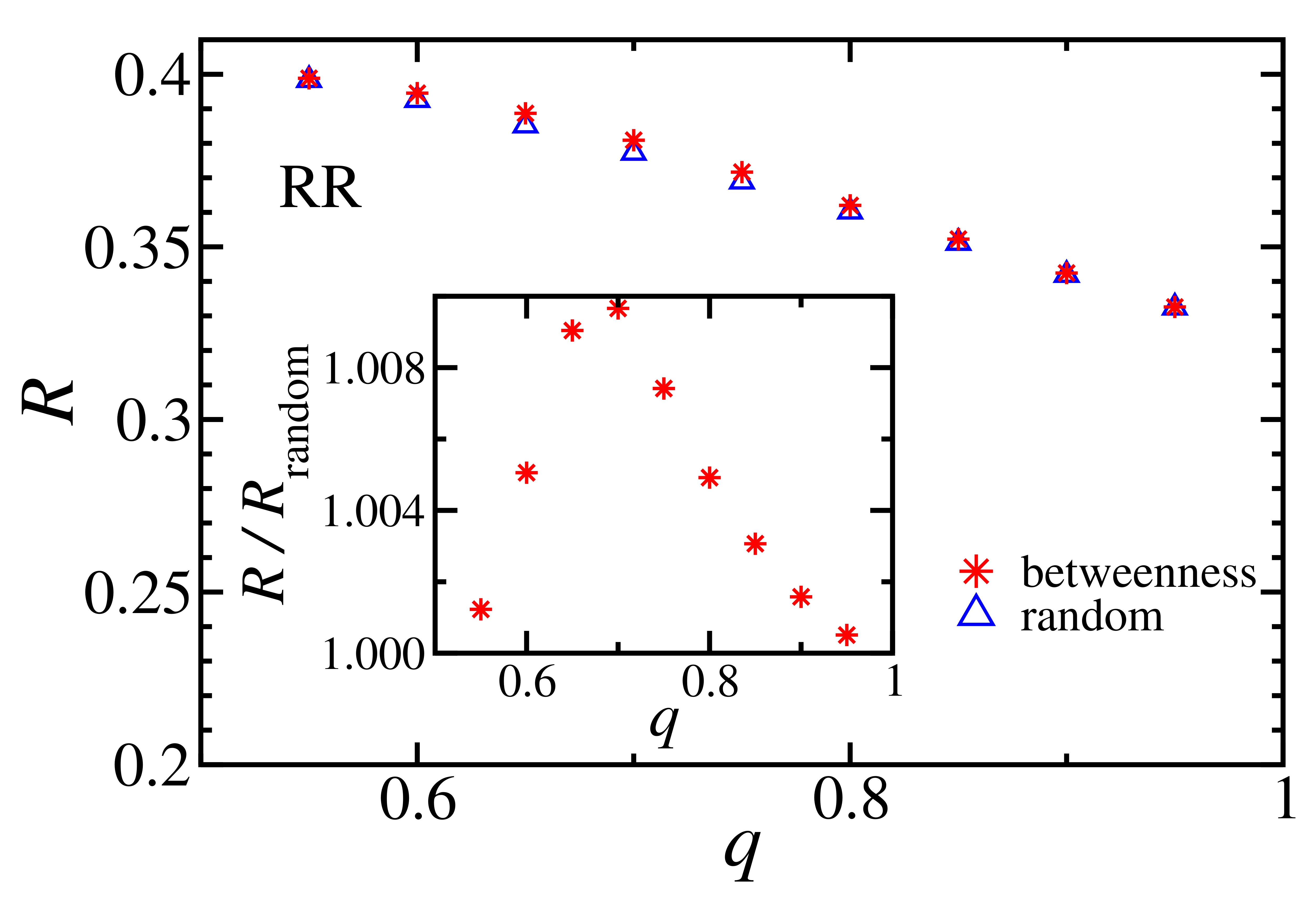
Another example that shows that betweenness is superior to degree is when we study coupled random regular graphs. In random regular graphs all nodes have the same degree and are connected randomly. Figure 6 shows the dependence of the robustness on the degree of coupling, for two interconnected random regular graphs with degree $4$. The autonomous nodes are selected randomly (since all degrees are the same) or following the betweenness strategy. Though all nodes have the same degree and the betweenness distribution is narrow, selecting autonomous nodes based on the betweenness is always more efficient than the random selection. Thus, the above two examples suggest that betweenness is a superior method to chose the autonomous nodes compared to degree.

Figure 7: Two-parameter diagram (blue curves) of two coupled ER (average degree $\langle k\rangle=4$) under random attack. The horizontal axis is the degree of coupling $q$ and the vertical one is $p$ so that $1-p$ is the fraction of initially removed nodes. The size of the jump in the fraction of $A$-nodes in the largest connected cluster is also included (red-dotted-dashed curve). The dashed curve stands for a discontinuous transition while the solid one is a critical line (continuous transition). The two lines meet at a tricritical point (TP). Autonomous nodes are selected based on the degree (main plot) and randomly (inset). Results have been obtained with the formalism of generating functions.

Figure 8: Tricritical coupling $q_{t}$ dependence on the average degree $\langle k\rangle$ for two coupled ER, showing that the fraction of autonomous nodes to smoothen out the transition is significantly reduced with the proposed strategy when compared with the random case. Autonomous nodes are selected following two different strategies: randomly (red squares) and high degree (black circles).

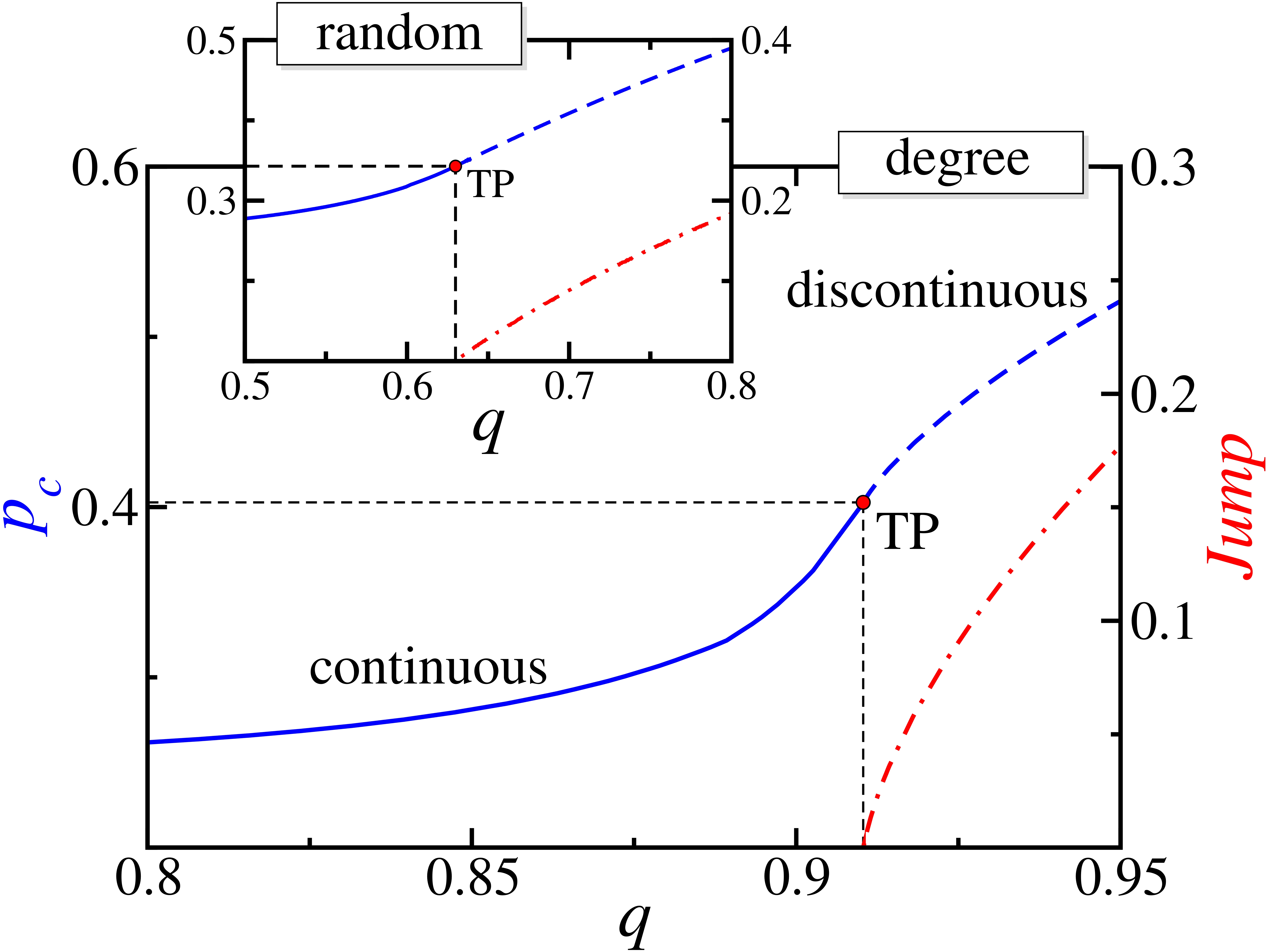
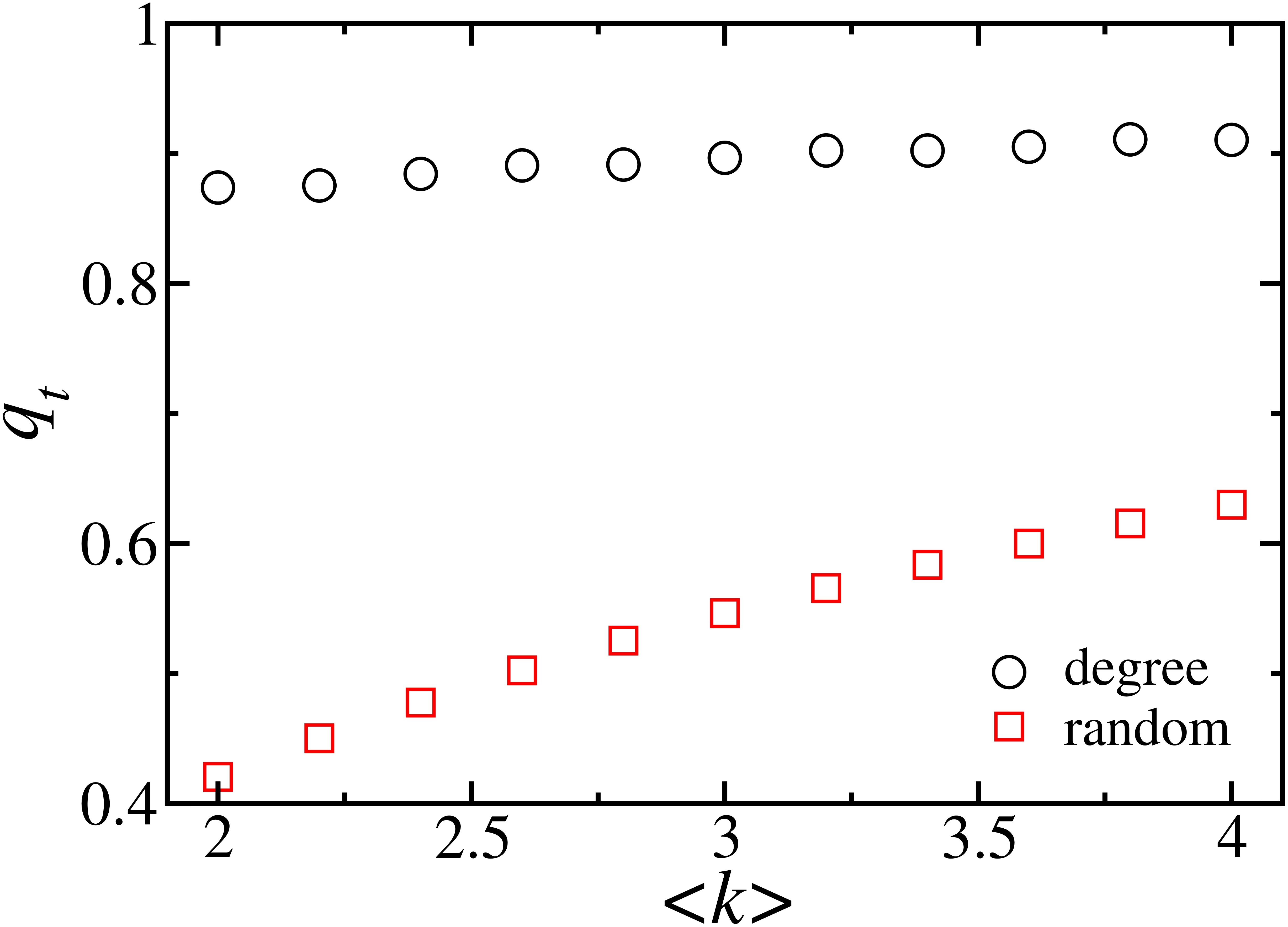
The vulnerability is strongly related to the degree of coupling $q$. Parshani et al. Parshani10 have analytically and numerically shown that, for random coupling, at a critical coupling $q=q_{t}$, the transition changes from continuous (for $q<q_{t}$) to discontinuous (for $q>q_{t}$). In Fig. 7 we see the two-parameter diagram ($p_{c}$ vs $q$) with the tricritical point and the transition lines (continuous and discontinuous) for the random (inset) and the degree (main) strategies. As seen in Fig. 7, when autonomous nodes are randomly selected, about $40\%$ autonomous nodes are required to soften the transition and avoid catastrophic cascades, while following the strategy proposed here only a relatively small amount ($q>0.9$) of autonomous nodes are needed to avoid a discontinuous collapse. Above the tricritical point, the jump increases with the degree of coupling, lending arguments to the paramount necessity of an efficient strategy for autonomous selection, given that the fraction of nodes which can be decoupled is typically limited. The dependence of $q_{t}$ on the average degree $\langle k\rangle$ is shown in Fig. 8. The ratio between the tricritical coupling for degree and random strategies increases with decreasing $\langle k\rangle$. For example, for $\langle k\rangle\approx 2$ the fraction of autonomous nodes needed to soften the transition with the random selection is six times the one for the degree strategy.

Figure 9: Dependence of the fraction of $A$-nodes in the largest connected cluster on the scaling field $\mu_{p}$ along the direction perpendicular to the transition line at the tricritical point. The slope is the tricritical exponent $\beta_{t}$ related with the order parameter. Autonomous nodes in the two coupled ER ($\langle k\rangle=4$) have been selected randomly (red line) and following the ranking of degree (black line).

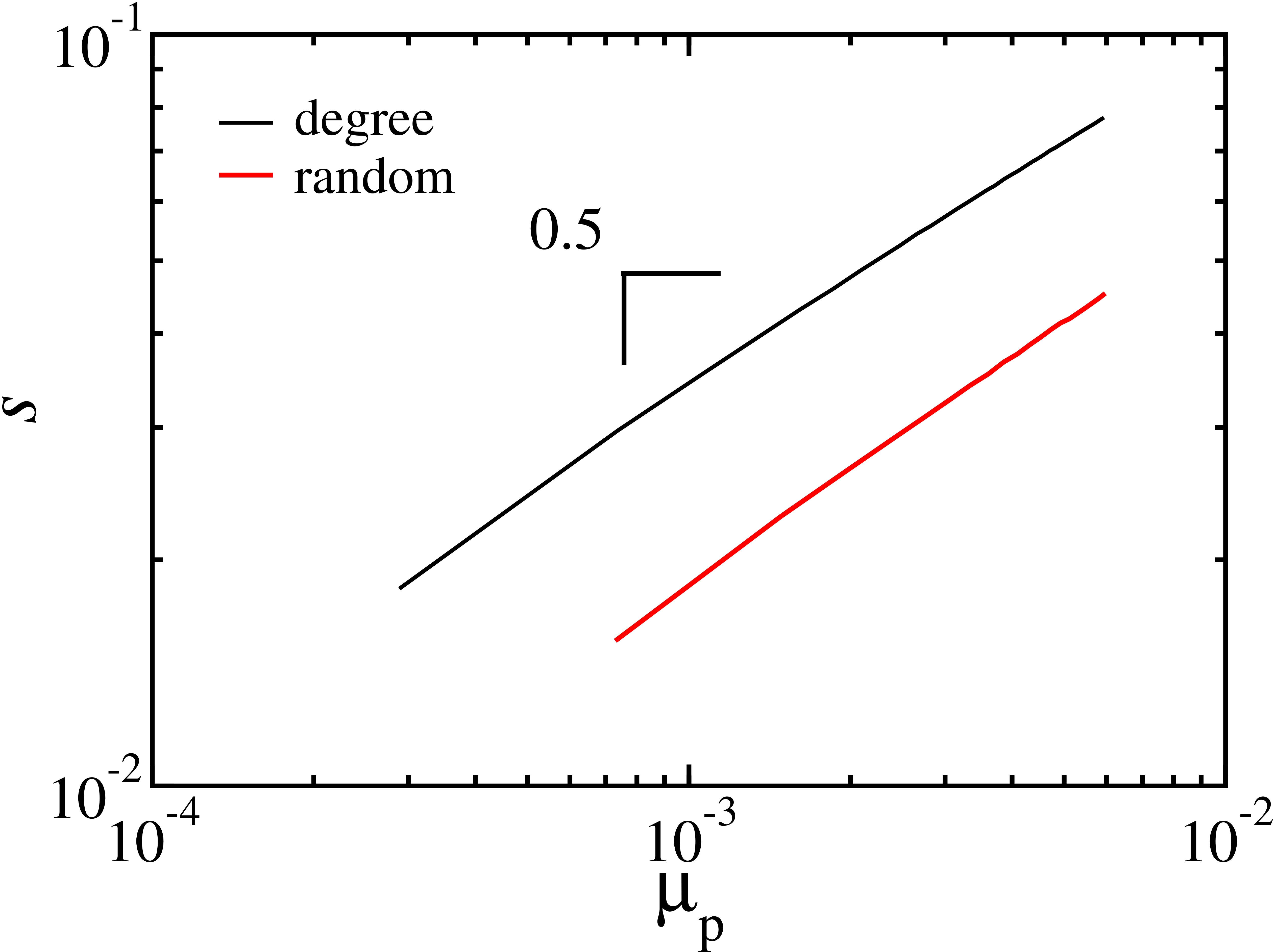
As in Ref. Araujo11 , following the theory of Riedel and Wegner Riedel69 ; Riedel72 ; Riedel72b , we can characterize the tricritical point. Two relevant scaling fields are defined: one tangent ($\mu_{p}$) and the other perpendicular ($\mu_{q}$) to the critical curve at the tricritical point. In these coordinate axes the continuous line is described by $\mu_{p}\sim\mu_{q}^{1/\varphi_{t}}$, where the tricritical crossover exponent $\varphi_{t}=1.00\pm 0.05$ for degree and random strategies. The tricritical order parameter exponent, $\beta_{t}$, can be evaluated from,

$$s\left(\mu_{p},\mu_{q}=0\right)\sim\mu_{p}^{\beta_{t}},$$ (4)

giving $\beta_{t}=0.5\pm 0.1$ for both strategies. Since these two exponents are strategy independent (see Fig. 9), we conjecture that the tricritical point for degree and random selection are in the same universality class.

Discussion

Here, we propose a method to chose the autonomous nodes in order to optimize the robustness of coupled networks to failures. We find the betweenness and the degree to be the key parameters for the selection of such nodes and we disclose the former as the most effective for modular networks. Considering the real case of the Italian communication network coupled with the power grid, we show in Fig. 1 that protecting only the four communication servers with highest betweenness reduces the chances of catastrophic failures like that witnessed during the blackout in 2003. When this strategy is implemented the resilience to random failures or attacks is significantly improved and the fraction of autonomous nodes necessary to change the nature of the percolation transition, from discontinuous to continuous, is significantly reduced. We also show that, even for networks with a narrow distribution of node degree like Erdős-Rényi graphs, the robustness can be significantly improved by properly choosing a small fraction of nodes to be autonomous. As a follow-up it would be interesting to understand how correlation between nodes, as well as dynamic processes on the network, can influence the selection of autonomous nodes. Besides, the cascade phenomena and the mitigation of vulnerabilities on regular lattices and geographically embedded networks are still open questions. It is important to note that while we use here high betweenness and high degree as a criterion for autonomous nodes, it is possible that other metrics will be also useful. For example, the eigenvector component of the largest eigenvector of the adjacency matrix (even weighted) makes a very good candidate (see e.g. vanMieghem11 ).

Methods

We consider two coupled networks, $A$ and $B$, where a fraction of $1-p$ $A$-nodes fails. The cascade of failures can be described by the iterative equations, Eqs. (2) Buldyrev10 ; Parshani10 , where $\alpha_{n}$ and $\beta_{n}$ are, respectively, the fraction of $A$ and $B$ surviving nodes at iteration step $n$ (not necessarily in the largest component), and $S_{x}(\chi_{n})$ ($\chi=\alpha|\beta$, $x=A|B$) is the fraction of nodes in the largest component in network $x$ given that $1-\chi$ nodes have failed. This can be calculated for coupled networks in the thermodynamic limit ($N\rightarrow\infty$) using generating functions.

Random Protection

As proposed by Parshani et al. Parshani10 , when autonomous nodes are randomly selected and the degree of coupling is the same in $A$ and $B$, the set of Eqs. (2) simplifies to

$$\alpha_{1} = p,$$

$$\beta_{n} = 1-q\left[1-S_{A}(\alpha_{n})p\right],$$ (5)

$$\alpha_{n} = p\left(1-q\left[1-S_{B}(\beta_{n-1})\right]\right),$$

where $q$ is the degree of coupling. The degree distribution of the networks does not change in the case of random failures and $S_{x}(\chi_{n})$ can be calculated as $S_{x}(\chi)=1-G_{P_{x}}\left(1-\chi(1-u_{x})\right)$ Newman02 , where $G_{P_{x}}(z)$ is the generating function of the degree distribution of network $x$,

$$G_{P_{x}}(z)=\sum_{k}{P_{x}(k)z^{k}},$$

and $u_{x}$ satisfies the transcendental equation

$$u_{x}=\frac{G^{\prime}_{P_{x}}\left(1-\chi(1-u_{x})\right)}{G^{\prime}_{P_{x}}(1)}.$$

The size of the largest component in network $x$ is given by $\chi S_{x}(\chi)$.

For ER networks $G_{P_{x}}(y)=\exp\left[\left<k\right>_{x}(z-1)\right]$, where $\left<k\right>_{x}$ is the average number of links in network $x$, and therefore

$$\frac{G^{\prime}_{P_{x}}\left(y\right)}{G^{\prime}_{P_{x}}(1)}=G_{P_{x}}(y).$$

With the above equations one can calculate the size of the largest component in both networks at the end of the cascade process.

Recently, Son et al. Son11b proposed an equivalent scheme based on epidemic spreading to solve the random protection case.

High Degree Protection

When autonomous nodes are selected following the degree strategy, the fraction of dependent nodes $q_{xn}$ changes with the iteration step $n$ and the set of Eqs. 2 no longer simplifies. We divide the discussion below into three different parts: the degree distribution, the largest component, and the coupling (fraction of dependent nodes).

The Degree Distribution

The networks A and B are characterized by their degree distributions, $P_{A}(k)$ and $P_{B}(k)$, which are not necessarily the same. The developed formalism applies to any arbitrary degree distribution. We start by first splitting the degree distribution into two parts, the component corresponding to the low-degree dependent nodes, $P_{xD}(k)$, and the component corresponding to the high-degree autonomous ones, $P_{xI}(k)$. To accomplish this, one must determine two parameters, the maximum degree of dependent nodes, $k_{xm}$, and the fraction of nodes with degree $k_{xm}$ that are coupled with the other network, $f_{xm}$. These two parameters can be obtained from the relations,

$$\sum_{k=0}^{k_{xm}-1}{P_{x}(k)}<q<\sum_{k=0}^{k_{xm}}{P_{x}(k)}$$

and

$$\sum_{k=0}^{k_{xm}-1}{P_{x}(k)}+f_{xm}P_{x}(k_{xm})=q,$$

where $q_{x}$ is the initial degree of coupling. One can then write

$$P_{xD}(k)=\left\{\begin{array}[]{ll}P_{x}(k),&k<k_{xm}\\ f_{xm}P_{x}(k),&k=k_{xm}\\ 0,&k>k_{xm}\end{array}\right.$$ (6)

and

$$P_{xI}(k)=\left\{\begin{array}[]{ll}0,&k<k_{xm}\\ (1-f_{xm})P_{x}(k),&k=k_{xm}\\ P_{x}(k),&k>k_{xm}\end{array}.\right.$$ (7)

In the model, a fraction of $1-p$ $A$-nodes are randomly removed. If, at iteration step $n$, $\alpha_{n}$ nodes survive ($\alpha_{n}\leq p$), $p(1-q_{A})$ nodes are necessarily autonomous and the remaining ones, $\alpha_{n}-p(1-q_{A})$, are dependent nodes. One can then show that the degree distribution of network $A$, under the failure of $1-\alpha_{n}$ nodes, $P^{\prime}_{A,n}(k)$, is given by

$$P_{A,n}^{\prime}(k)=\left(\frac{1-\frac{p}{\alpha_{n}}(1-q)}{q}\right)P_{AD}(k)+\frac{p}{\alpha_{n}}P_{AI}(k),$$

while the fraction of surviving links is

$$p_{An}=\alpha_{n}\frac{\sum_{k}{kP_{A,n}^{\prime}(k)}}{\sum_{k}{kP_{A}(k)}}.$$

All the $B$-nodes which do not survive are dependent and so the degree distribution at iteration $n$, $P_{B,n}^{\prime}(k)$, is given by

$$P_{B,n}^{\prime}(k)=\left(\frac{1-\frac{1}{\beta_{n}}(1-q)}{q}\right)P_{BD}(k)+\frac{1}{\beta_{n}}P_{BI}(k),$$

while the fraction of surviving links is

$$p_{Bn}=\beta_{n}\frac{\sum_{k}{kP_{B,n}^{\prime}(k)}}{\sum_{k}{kP_{B}(k)}}\ \ .$$

The Largest Component

With the degree distribution $P_{x,n}^{\prime}(k)$ and the fraction of surviving links $p_{xn}$ one can calculate the size of the largest component as

$$S_{x}(\chi_{n}) = 1-G_{P^{\prime}_{xn}}\left(1-p_{xn}+p_{xn}\tau_{xn}\right)$$

$$= 1-\sum_{k}{P_{xn}^{\prime}(k)\left(1-p_{xn}+p_{xn}\tau_{xn}\right)^{k}},$$

where $\tau_{xn}$ satisfies the self consistent equation

$$\tau_{xn} = \frac{G^{\prime}_{P^{\prime}_{xn}}\left(1-p_{xn}+p_{xn}\tau_{xn}\right)}{G^{\prime}_{P^{\prime}_{xn}}(1)}$$

$$= \frac{\sum_{k}{kP_{xn}^{\prime}(k)\left(1-p_{xn}+p_{xn}\tau_{xn}\right)^{k-1}}}{\sum_{k}{kP_{xn}^{\prime}(k)}}.$$

The coupling

To calculate the fraction $q_{\alpha,n}$ (and $q_{\beta,n}$) one must first calculate the degree distribution of the nodes in the largest component. This is given by

$$P_{xG,n}(k)=P_{xn}^{\prime}(k)\frac{1-\left(1-p_{xn}+p_{xn}\tau_{xn}\right)^{k}}{S_{\chi_{n}x}(\chi_{n})}.$$

The fraction of nodes in the largest component that are autonomous is then given by

$$q_{xG,n}=\left(1-f_{xm}\right)P_{xG,n}(k_{xm})+\sum_{k=k_{xm}+1}^{\infty}{P_{xG,n}(k)},$$

where the upper limit of the sum is the maximum degree in the network, which we consider to be infinity in the thermodynamic limit. The fraction of autonomous nodes from the original network remaining in the largest component is $q_{xG,n}\chi_{n}S_{x}(\chi_{n})$, while the total fraction of autonomous nodes is given by $1-q$. The fraction of nodes disconnected from the largest component that are autonomous is then given by

$$1-q_{x,n}=\frac{1-q-q_{xG,n}\chi_{n}S_{x}(\chi_{n})}{1-\chi_{n}S_{x}(\chi_{n})},$$

so that the fraction of dependent nodes which have fragmented from the largest component is

$$q_{x,n}=1-\frac{1-q-q_{xG,n}\chi_{n}S_{x}(\chi_{n})}{1-\chi_{n}S_{x}(\chi_{n})}.$$

For simplicity, here we assume that $k_{x,m}$ and $f_{xm}$ are constant and do not change during the iterative process. In fact, this is an approximation as the degree of the autonomous nodes is expected to change when their neighbors fail. However, in spite of shifting the transition point, this consideration does not change the global picture described here.

Numerical simulations

Numerical results have been obtained with the efficient algorithm described in Ref. Schneider13 for coupled networks.

References

- (1) Peerenboom, J., Fischer, R., and Whitfield, R. Recovering from disruptions of interdependent critical infrastructures. Pro. CRIS/DRM/IIIT/NSF Workshop Mitigat. Vulnerab. Crit. Infrastruct. Catastr. Failures (2001).
- (2) Rosato, V. et al. Modelling interdependent infrastructures using interacting dynamical models. Int. J. Crit. Infrastruct. 4, 63 (2008).
- (3) Schweitzer, F. et al. Economic networks: The new challenges. Science 325, 422 (2009).
- (4) Buldyrev, S. V. et al. Catastrophic cascade of failures in interdependent networks. Nature 464, 1025 (2010).
- (5) Brummitt, C. D., D’Souza, R. M., and Leicht, E. A. Suppressing cascades of load in interdependent networks. Proc. Nat. Acad. of Sciences USA 109, E680 (2012).
- (6) Gao, J., Buldyrev, S. V., Stanley, H. E., and Havlin, S. Networks formed from interdependent networks. Nat. Phys. 8, 40 (2012).
- (7) Parshani, R., Buldyrev, S. V., and Havlin, S. Interdependent networks: reducing the coupling strength leads to a change from a first to second order percolation transition. Phys. Rev. Lett. 105, 048701 (2010).
- (8) Son, S.-W. et al. Percolation theory on interdependent networks based on epidemic spreading. EPL 97, 16006 (2012).
- (9) Huang, X. et al. Robustness of interdependent networks under targeted attack. Phys. Rev. E 83, 065101(R) (2011).
- (10) Schneider, C. M. et al. Mitigation of malicious attacks on networks. Proc. Nat. Acad. Sci. 108, 3838 (2011).
- (11) Herrmann, H. J. et al. Onion-like network topology enhances robustness against malicious attacks. J. Stat. Mech. , P01027 (2011).
- (12) Parshani, R. et al. Inter-similarity between coupled networks. EPL 92, 68002 (2010).
- (13) Buldyrev, S. V., Shere, N. W., and Cwilich, G. A. Interdependent networks with identical degrees of mutually dependent nodes. Phys. Rev. E 83, 016112 (2011).
- (14) Newman, M. E. J. Networks: An Introduction. Oxford University Press, Oxford, (2010).
- (15) Carmi, S. et al. A model of internet topology using k-shell decomposition. Proc. Natl. Acad. Sci. USA 104, 11150 (2007).
- (16) Albert, R., Jeong, H., and Barabási, A.-L. Error and attack tolerance of complex networks. Nature 406, 378 (2000).
- (17) Clauset, A., Shalizi, C. R., and Newman, M. E. J. Power-law distributions in empirical data. SIAM Rev. 51, 661 (2009).
- (18) Cohen, R. and Havlin, S. Complex Networks: Structure, Robustness and Function. Cambridge University Press, United Kingdom, (2010).
- (19) Ravasz, E. et al. Hierachical organization of modularity in metabolic networks. Science 297, 1551 (2002).
- (20) Happel, B. L. M. and Murre, J. M. J. Design and evolution of modular neural-network architectures. Neural Netw. 7, 985 (1994).
- (21) González, M. C., Herrmann, H. J., Kertész, J., and Vicsek, T. Community structure and ethnic preferences in school friendship networks. Physica A 379, 307 (2007).
- (22) Eriksen, K. A., Simonsen, I., Maslov, S., and Sneppen, K. Modularity and extreme edges of the internet. Phys. Rev. Lett. 90, 148701 (2003).
- (23) Araújo, N. A. M., Andrade Jr., J. S., Ziff, R., and Herrmann, H. J. Tricritical point in explosive percolation. Phys. Rev. Lett. 106, 095703 (2011).
- (24) Riedel, E. K. and Wegner, F. Scaling approach to anisotropic magnetic systems statics. Z. Physik 225, 195 (1969).
- (25) Riedel, E. K. Scaling approach to tricritical phase transitions. Phys. Rev. Lett. 28, 675 (1972).
- (26) Riedel, E. K. and Wegner, F. J. Tricritical exponents and scaling fields. Phys. Rev. Lett. 29, 349 (1972).
- (27) Newman, M. E. J. Spread of epidemic disease on networks. Phys. Rev. E 66, 016128 (2002).
- (28) van Mieghem, P. et al. Decreasing the spectral radius of a graph by link removals. Phys. Rev. E 84, 016101 (2011).
- (29) Schneider, C. M., Araújo, N. A. M., and Herrmann, H. J. Efficient algorithm to study interconnected networks. Phys. Rev. E 87, 043302 (2013).