Homogenization of Metamaterials by Dual Interpolation of Fields:
a Rigorous Treatment of Resonances and Nonlocality

Abstract. The paper extends and enhances in several ways the recently proposed homogenization theory of metamaterials [J. Opt. Soc. Am. B 28, 577 (2011)]. The theory is based on a direct analysis of fields in the lattice cells rather than on an indirect retrieval of material parameters from transmission / reflection data. The theory is minimalistic, with only two fundamental premises at its core: (i) the coarse-grained fields satisfy Maxwell’s equations and boundary conditions exactly; and (ii) the material tensor is a linear relationship between the pairs of coarse-grained fields. There are no heuristic assumptions and no artificial averaging rules. Nontrivial magnetic behavior, if present, is a logical consequence of the theory. The method yields not only all 36 standard material parameters, but also additional ones quantifying spatial dispersion rigorously. The approximations involved are clearly identified. A tutorial example and an application to a resonant structure with high-permittivity inclusions are given.

1 Introduction

The complex electromagnetic behavior of metamaterials – artificial periodic structures with features smaller than the vacuum wavelength – has been extensively investigated over the last decade. One particularly intriguing phenomenon is “artificial magnetism” at high frequencies. A physical explanation for it is that resonating elements in metamaterial cells act as elementary magnetic dipoles. However, there is a paradox associated with such magnetism. In a metamaterial composed of intrinsically nonmagentic components, the “microscopic” (pointwise) magnetic fields $\mathbf{h}$ and $\mathbf{b}$ are the same; yet somehow their spatial averages – the respective coarse-grained fields $\mathbf{H}$ and $\mathbf{B}$ – differ. How can two identical quantities give rise to two different averages?

The theory proposed in [2] resolves this paradox. A key observation – critical from both mathematical and physical viewpoints – is that, for Maxwell’s equations and standard boundary conditions to be honored, the coarse-grained fields $\mathbf{H}$ and $\mathbf{B}$ must be obtained from $\mathbf{b}$ via different interpolation procedures. Indeed, $\mathbf{H}$ has tangential continuity across all interfaces whereas $\mathbf{B}$ has normal continuity. Specific interpolation procedures producing fields with the required types of continuity are discussed in [2] and are, for the sake of completeness, reviewed in Section 3.

The theory of [2], significantly extended and enhanced in the present paper, has several distinguishing features. First, it is based on a direct analysis of the field in the lattice cell. This is in contrast with S-parameter retrieval procedures [3]–[7] where the effective parameters are inferred from reflection and transmission coefficients of a metamaterial slab. Second, the theory is minimalistic, with only two fundamental premises at its core: (i) the coarse-grained fields must satisfy Maxwell’s equations and boundary conditions; and (ii) the material tensor is a linear relationship between the pairs of coarse-grained fields $(\mathbf{E},\mathbf{H})$ and $(\mathbf{D},\mathbf{B})$. There are no heuristic assumptions and no artificial averaging rules contrived to arrive at a desired result such as magnetic permeability $\mu\neq 1$; nontrivial magnetic behavior, if present, follows logically from the method, along with other essential characteristics and effects. Third, not only all 36 standard material parameters, but also additional ones quantifying spatial dispersion can be found, as explained in Sect. 3, 4.

The effective medium description of metamaterials is, despite very intensive studies, still far from being settled in a rigorous way. The existing literature on this subject is quite vast, and the approaches include retrieval via S-parameters, applications and extensions of classical mixing formulas for small inclusions, analysis of dipole lattices, special current-driven models, and much more. Reviews and references are available in [8]–[10] and a recent summary can be found in the Introduction of [18, 2]. Here I summarize only two approaches most relevant to the present paper.

In one common procedure already noted, effective parameters of a metamaterial slab are “retrieved” from transmission/reflection data (i.e. from S-parameters). Being essentially an inverse problem, this parameter retrieval has some inherent ill-posedness that manifests itself in the multiplicity of solutions, due to the ambiguity of branches of the inverse trigonometric functions involved. Parameters obtained from transmission/reflection from slabs of varying thickness (let alone shape) are not always consistent. More fundamentally, the retrieval procedure does not by itself explain why such consistency should be expected; obviously, there must be an underlying reason for it. That deeper reason is the definition of material parameters as relations between the (pairs of) coarse-grained fields.

The existing approach most closely related to the methodology of the present paper is due to the insight of Smith & Pendry, who suggested different averaging procedures for different fields in the cell [21]. Their justification came from the analogy with finite difference schemes on staggered grids. The present paper, along with [2], provides a substantially more rigorous foundation for this physical insight and a much more comprehensive description of the behavior of the fields in terms of the $6\times 6$ parameter matrix and beyond.

The key concepts of the proposed theory are familiar to applied mathematicians and numerical analysts, but their application to homogenization and metamaterials is novel. For this reason, the exposition below is split into several parts: a general description of the key concepts, followed by some technical details, implementation and examples.

2 Proposed Theory: Key Concepts

The proposed theory follows directly and logically from the definition of material parameters as linear relations between the coarse-grained fields. Naturally, this requires these coarse-grained fields to be unambiguously defined and relations between them established. That is the main theme of this paper.

The motivation for any effective medium theory is that the microscopic fields vary too rapidly to be easily described and analyzed; one may say that they have “too many degrees of freedom”. An obvious idea is to split them up into coarse-grained (capital letters) and fast (tilde-letters) components, e.g. $\mathbf{b}=\mathbf{B}+\mathbf{b}^{\sim}$. For reasons explained in detail below, this splitting should satisfy several conditions:

1. By definition, the coarse-grained fields must vary much less rapidly than the total fields. Nevertheless the coarse-grained fields must approximate, in a certain well defined sense, the actual physical fields everywhere in space.

2. The coarse-grained fields must satisfy Maxwell’s equations and interface boundary conditions.

3. The fast and coarse components must be semi-decoupled, in the following sense. The fast components may depend on the coarse ones, but the coarse fields must not depend, or may depend only very weakly, on the fast ones.

4. There exists a linear relationship between the pairs of coarse-grained fields $(\mathbf{E},\mathbf{H})$ and $(\mathbf{D},\mathbf{B})$ that is independent of the incident waves (at least to a given level of approximation).

The requirements above define not a single method but a framework from which conceptually similar but not fully equivalent homogenization methods could potentially be obtained by making these requirements more specific.

The rationale for each of the conditions above is as follows. The first one represents, from the physical perspective, the very essence of homogenization. From a more mathematical viewpoint of analysis and simulation, one might accept a weaker requirement that the coarse fields can be described with much fewer degrees of freedom than the total fields; the coarse fields would not necessarily have to vary less rapidly. For example, the field in a periodic structure can in many cases be described by a very limited number of Bloch waves with judiciously chosen wave vectors (see e.g. [11] for some illuminating examples); this fact may be effectively used in semi-analytical and numerical methods such as Generalized Finite Element Method (GFEM) [12]–[14], Discontinuous Galerkin methods [15], and Flexible Local Approximation MEthods (FLAME) [33, 34, 32]. Nevertheless the focus of this paper is on the methods that could give maximum physical insight via traditional electromagnetic parameters.

Pointwise approximation of the miscorscopic fields by the coarse ones is in general not feasible and not required, as rapid local field oscillations due to the resonance effects in metamaterial cells are definitely of interest. Instead, we assume that the coarse-grained fields are close to the real ones at the cell boundary, where the fields vary more smoothly. Inside the cell, the coarse-grained fields are defined by interpolation from the boundary values.

Although the second requirement (coarse-grained fields satisfying Maxwell’s equations) seems to be perfectly natural, many existing methods pay surprisingly little attention to it and may actually violate it. In particular, coarse fields defined via simple volume averaging do not satisfy Maxwell’s boundary conditions. We shall return to this important point later.

The rationale for the third requirement (weak coupling) is that, if both components were to be coupled strongly, the two-scale problem would not be any simpler than the original one involving the total field.

The fourth requirement is for now open-ended and needs to be made more specific. Let us assume that, for a given microscopic field $(\mathbf{e},\mathbf{d},\mathbf{b})$, the coarse-grained fields $(\mathbf{E},\mathbf{D},\mathbf{B},\mathbf{H})$ satisfying conditions 1–3 above have been defined in some way. The central question then is to relate the pairs of coarse-grained fields. The generalized “material parameter” is, mathematically, a linear map $\mathcal{L}:(\mathbf{E}$, $\mathbf{H})\rightarrow(\mathbf{D},\mathbf{B})$ from the functional space of fields $(\mathbf{E}$, $\mathbf{H})$ to the functional space of $(\mathbf{D},\mathbf{B})$. The dimensionality of this map depends on the coarse-grained interpolations chosen. A high-dimensional linear map could be of use in numerical procedures but does not offer much physical insight. One critical question then is whether a good low-dimensional – mathematically, a low-rank – approximation of this linear map can be found. A pure linear-algebraic answer to this question is well known: the best approximation of a given rectangular matrix by a matrix of rank $m$ is via the highest $m$ singular values and the respective singular vectors (see e.g. [16] or [17] for the mathematical details). The error of this approximation is equal to the $m+1$st singular value. One may note a conceptual similarity with the well known Principal Component Analysis (PCA); see e.g. [35] for an elementary tutorial.

Although the PCA perspective is instructive, it does not provide a direct connection with the physical parameters such as $\epsilon$ or $\mu$. Our objective is still to find new bases in which the material map $\mathcal{L}$ could be “compressed” to a low-dimensional form, but the bases we are seeking are physical rather than formally algebraic. More specifically, in this physical basis the first few components of the coarse-grained fields $\mathbf{E},\mathbf{H},\mathbf{D},\mathbf{B}$ are to be their mean values, and the subsequent components – the increments of these fields. Such bases and the respective matrix representation of the map $\mathcal{L}$ will be called canonical; see Section 3 for details.

3 Proposed Theory: Details

3.1 Equations

Consider a periodic structure composed of materials that are assumed to be (i) intrinsically nonmagnetic (which is true at sufficiently high frequencies [24]); (ii) satisfy a linear local constitutive relation $\mathbf{d}=\epsilon\mathbf{e}$. For simplicity, we assume a cubic lattice with cells of size $a$.

Maxwell’s equations for the microscopic fields are, in the frequency domain and with the $\exp(-\mathrm{i}\omega t)$ phasor convention,

$$\nabla\times\mathbf{e}=\mathrm{i}\omega c^{-1}\mathbf{b},~{}~{}~{}\nabla\times\mathbf{b}=-\mathrm{i}\omega c^{-1}\mathbf{d}$$

As in [2], small letters $\mathbf{b},\mathbf{e},\mathbf{d}$, etc., will denote the “microscopic” – i.e. true physical – fields that in general vary rapidly as a function of coordinates. Capital letters will refer to smoother fields, to be defined precisely later, that vary on the scale coarser than the lattice cell size.

The coarse-grained fields $\mathbf{B}$, $\mathbf{H}$, $\mathbf{E}$, $\mathbf{D}$ must be defined in such a way that the boundary conditions be honored. As noted in [2], simple cell-averaging does not satisfy this condition. To understand why, consider, say, the “microscopic” magnetic field, for simplicity just a function of one coordinate, $\mathbf{b}(x)$, at a material/air interface $x=0$. For intrinsically nonmagnetic media, this field is continuous across the interface, i.e. $\mathbf{b}(x=0-)=\mathbf{b}(x=0+)$. Since the field fluctuates in the material, there is no reason for its value at $x=0$ to be equal to its cell average over $0\leq x\leq a$. Thus, if this cell average is used to define the $\mathbf{B}$ field, its normal component at the interface will in virtually all cases be discontinuous, which is nonphysical. Likewise, if the $\mathbf{H}$ field is defined via the cell average, its tangential component will in general behave in a nonphysical way.

As a rough, “zero-order,” approximation, these nonphysical field jumps across the interface could be neglected. This may indeed be possible in the absence of resonances or for vanishingly small cell sizes. However, neglecting strong field fluctuations in other cases would eliminate the very resonance effects that we are trying to describe.

To help the reader navigate the proposed procedure without getting bogged down in technical detail, let us review the general stages of the method (Fig. 1) and explain why each of them is necessary. The core of the theory proposed in [2] – tangentially- and normally-continuous interpolations, as well as approximation of the field as a linear combination of basis functions (modes) – remains intact, but the “inner workings” of various components have been modified, as explained in the subsequent sections.

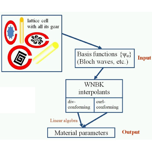
Figure 1: Key parts of the proposed methodology. Two types of interpolation are used to obtain the coarse-grained fields with tangential and normal continuity. The electromagnetic field inside the cell, with all its microstructure, is approximated with a set of basis modes. Material parameters are linear-algebraic relationships between the pairs of coarse-grained fields.

3.2 Coarse-grained fields: interpolation and continuity conditions

This is the central point of the proposed methodology, where we depart from more traditional methods of field averaging. The coarse-grained $\mathbf{E}$ and $\mathbf{H}$ fields are produced from the “microscopic” ones, $\mathbf{e}$ and $\mathbf{b}$, by an interpolation that respects tangential continuity across all interfaces. The coarse-grained $\mathbf{D}$ and $\mathbf{B}$ fields are produced from $\mathbf{d}$ and $\mathbf{b}$ by another interpolation, one that preserves normal continuity.

Tangentially continuous interpolation is effected by vectorial functions like the one shown in Fig. 2, in a 2D rendition for simplicity. The circulation of this function is equal to one along one edge (in the figure, the vertical edge shared by two adjacent lattice cells) and zero along all other edges of the lattice.

To shorten all interpolation-related expressions, in this section the lattice cell is normalized to the unit cube $[0,1]^{3}$, i.e. $a=1$. Then a formal expression for four $x$-directed functions $\mathbf{w}$ is

$$\mathbf{w}_{1-4}=2\hat{x}\{yz,(1-y)z,y(1-z),(1-y)(1-z)\}$$ (1)

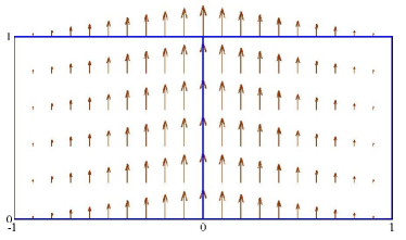
Figure 2: (From [Tsukerman, J Opt Soc Am B, 28, 2011].) A 2D analog of the vectorial interpolation function $\mathbf{w}_{\alpha}$ (in this case, associated with the central vertical edge shared by two adjacent cells). Tangential continuity of this function is evident from the arrow plot; its circulation is equal to one over the central edge and to zero over all other edges.

Another eight functions of this kind are obtained by the cyclic permutation of coordinates in the expression above. For each lattice cell, there are 12 such interpolating functions altogether (one per edge). Each function $\mathbf{w}_{\alpha}$ has unit circulation along edge $\alpha$ ($\alpha=1,2,\ldots 12$) and zero circulations along all other edges. All of them are vectorial interpolating functions, bilinear with respect to the spatial coordinates. (In [2] these functions were defined in the cell scaled to $[-1,1]^{3}$ rather than to $[0,1]^{3}$, and therefore the algebraic expressions differ.)

The coarse-grained $\mathbf{E}$ and $\mathbf{H}$ fields can then be represented by interpolation from the edges into the volume of the cell as follows:

$$\mathbf{E}~{}=~{}\sum\nolimits_{\alpha=1}^{12}\,[\mathbf{e}]_{\alpha}\mathbf{w}_{\alpha},~{}~{}\mathbf{H}~{}=~{}\sum\nolimits_{\alpha=1}^{12}\,[\mathbf{b}]_{\alpha}\mathbf{w}_{\alpha}$$ (2)

where $[\mathbf{e}]_{\alpha}=\int_{\alpha}{\mathbf{e}\cdot\mathbf{dl}}$ is the circulation of the (microscopic) $\mathbf{e}$-field along edge $\alpha$; similarly for $[\mathbf{b}]_{\alpha}$. In the calculation of the circulations, integration along the edge is always assumed to be in the positive direction of the respective coordinate axis.

Now consider the second kind of interpolation that preserves the normal continuity and produces the $\mathbf{D},\mathbf{B}$ fields from $\mathbf{d}$ and $\mathbf{b}$. A typical interpolating function (2D rendition again for simplicity) is shown in Fig. 3. The flux of this function through a face shared by two adjacent cells is equal to one; the flux through all other faces is zero. Two such functions in the $x$-direction are (as before, for the cell size normalized to unity)

$$\mathbf{v}_{1-2}=\hat{x}\{x,1-x\}$$

and another four functions $\mathbf{v}_{3-6}$, in the $y$- and $z$-directions, are expressed similarly. These six functions can be used to define the coarse-grained $\mathbf{D}$ and $\mathbf{B}$ fields by interpolation from the six faces into the volume of the unit cell:

$$\mathbf{D}\,=\,\sum_{\beta=1}^{6}[[d]]_{\beta}\mathbf{v}_{\beta},~{}~{}~{}\mathbf{B}\,=\,\sum_{\beta=1}^{6}[[b]]_{\beta}\mathbf{v}_{\beta},$$ (3)

where $[[d]]_{\beta}=\int_{\beta}{\mathbf{d}\cdot\mathbf{dS}}$ is the flux of $\mathbf{d}$ through face $\beta$ ($\beta=1,2,\ldots,6$); similar for the $\mathbf{b}$ field. In the calculation of fluxes, it is convenient to take the normal to any face in the positive direction of the respective coordinate axis (rather than in the outward direction).

The coarse-grained $\mathbf{E}$ and $\mathbf{H}$ fields so defined have 12 degrees of freedom in any given lattice cell. From the mathematical perspective, these fields lie in the 12-dimensional functional space spanned by functions $\mathbf{w}_{\alpha}$; we shall keep the notation $W_{\mathrm{curl}}$ of [2] for this space: the ‘W’ honors Whitney [22] (see [2] for details and further references) and ‘curl’ indicates fields whose curl is a regular function rather than a general distribution. This implies, in physical terms, the absence of equivalent surface currents and the tangential continuity of the fields involved.

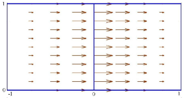
Figure 3: (From [Tsukerman, J Opt Soc Am B, 28, 2011].) A 2D analog of the vectorial interpolation function $\mathbf{v}_{\beta}$ (in this case, associated with the central vertical edge). Normal continuity of this function is evident from the arrow plot; its flux is equal to one over the central edge and zero over all other edges.

Similarly, $\mathbf{D}$ and $\mathbf{B}$ within any lattice cell lie in the six-dimensional functional space $W_{\mathrm{div}}$ spanned by functions $\mathbf{v}_{\beta}$. Importantly, it can be shown that the div- and curl-spaces are compatible in the following sense:

$$\nabla\times W_{\mathrm{curl}}\in W_{\mathrm{div}}$$ (4)

That is, the curl of any function from $W_{\mathrm{curl}}$ (i.e. the curl of any coarse-grained field $\mathbf{E}$ or $\mathbf{H}$ defined by (2)) lies in $W_{\mathrm{div}}$. Because of this compatibility of interpolations, the coarse-grained fields, as proved in [2], satisfy Maxwell’s equations exactly:

$$\nabla\times\mathbf{E}\,=\,\mathrm{i}\omega c^{-1}\mathbf{B};~{}~{}\nabla\times\mathbf{H}\,=\,-\mathrm{i}\omega c^{-1}\mathbf{D}$$ (5)

By construction, they also satisfy the proper continuity conditions at all interfaces. Thus the coarse-grained fields are completely physical.

To recap the ideas, Fig. 4 schematically illustrates the interpolation procedures and the linear-algebraic part of the proposed method. The simplified 1D rendition shows only the $x$ axis, the tangential ($y,z$) components of $\mathbf{E},\mathbf{H}$ and the normal ($x$) component of $\mathbf{D},\mathbf{B}$. Other components (not shown) may be discontinuous at cell boundaries and at material interfaces.

The linear relation $\mathcal{L}$ between the pairs of coarse-grained fields is in general multidimensional, commensurate with the dimensions of the interpolation spaces chosen. In “homogenizable” cases, $\mathcal{L}$ has a dominant $6\times 6$ (or smaller) matrix block in a suitable “canonical” basis; this block relates the field averages of $(\mathbf{D},\mathbf{B})$ to the field averages of $(\mathbf{E},\mathbf{H})$ . The remainder of the matrix relates the field averages to field variations over the cell and can be viewed as a manifestation of nonlocality (see Section 4 for further discussion).

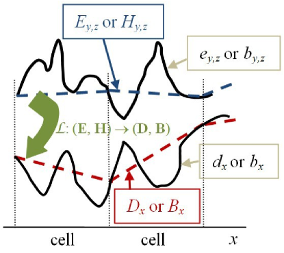
Figure 4: A linear relation between the coarse-grained fields. $\mathbf{E},\mathbf{H}$ are interpolated to ensure tangential continuity; $\mathbf{D},\mathbf{B}$ are normally continuous. 1D rendition for simplicity. The linear relation $\mathcal{L}$ between the pairs of fields is in general multidimensional but in “homogenizable” cases has a dominant $6\times 6$ (or smaller) block.

3.3 Approximating Functions

The actual microscopic fields in the material are in general not known and need to be approximated by introducing suitable basis functions [2]. For maximum generality, the choice of the basis is left open for now. Examples inclide Bloch waves in the periodic case, plane waves, cylindrical or spherical harmonics, etc. Although Bloch modes are very useful and physically meaningful, their use does have disadvantages and limitations. They are rigorously applicable only to periodic structures, which is strictly speaking not the case if the effective properties of the metamaterial need to vary – e.g. in cloaking applications. Evanescent field components are approximated by traveling Bloch waves very poorly, but these components are essential in imaging and other applications. In addition, Bloch modes are expensive to compute. An alternative set of basis functions that does not require eigenmodes is introduced below.

For a non-vanishing cell size, the field has an infinite number of degrees of freedom; thus, as a matter of principle, its representation in a finite basis is approximate. Nevertheless the relevant behavior of the fields can be captured very well by relatively small bases. By expanding the bases, one can increase the accuracy of the representation of the fields, at the expense of higher complexity. A small number of degrees of freedom corresponds to local material parameters, a moderately higher number – to nonlocal ones, and a large number falls under the umbrella of numerical simulation. This unifies local, nonlocal and numerical treatment of electromagnetic characteristics of metamaterials.

Note that tangential components of the electric or, alternatively, magnetic field on the cell boundary define the field inside the cell uniquely, except for the special cases of interior resonances. To specify the basis, it is thus sufficient to consider the boundary values in lieu of the values inside of the cell.

With all the above in mind, a rather natural set of approximating functions contains EM fields with the boundary values of $\mathbf{E}$ or $\mathbf{H}$ equal to those of the curl-conforming functions (1). In this setup, the approximating functions for the $\mathbf{e}$ and $\mathbf{b}$ fields on the cell boundary are the same as the interpolating functions for the coarse-grained fields $\mathbf{E},\mathbf{H}$. (The normally-continuous functions are still used for $\mathbf{D},\mathbf{B}$.)

Since the chosen interpolation functions are low-order polynomials, the accuracy of this approximation will depend on the smoothness of the field on the cell boundary and in general can be expected to depend on the size of the “buffer zone” between the inclusions in the cell and its boundary. However, effective parameters are essentially a zero-order approximation of the fields: a relationship between averaged fields that vary slowly within the cell. From this perspective, the low-order polynomial approximation on the boundary is unlikely to be a limiting factor in most practical cases.

The reader well versed in numerical analysis will immediately recognize that this type of interpolation is borrowed directly from edge elements in the finite element method (FEM), [23]. However, our goal is to develop an analytical rather than numerical procedure. It is curious, though not accidental, that the “numerical” tools of FEM prove to be quite suitable for analytical purposes as well.

It remains to decide whether the boundary values of the $\mathbf{e}$ field, $\mathbf{b}$ field or both will be taken as a basis for defining the approximating set. If one of the fields is chosen (either $\mathbf{e}$ or $\mathbf{b}$, arbitrarily), the number of approximating functions is equal to the number of curl-conforming functions (1), i.e. to 12. If both fields are chosen, there are 24 functions in the approximating set. In this latter case, some redundancy is apparent because the electric and magnetic fields are not independent. Nevertheless, for reasons of symmetry and elegance, it is convenient to use the 24-function set and deal with the redundancy later.

3.4 The Canonical Relation and Material Parameters

By construction of the coarse-grained interpolants, the $\mathbf{E}$ and $\mathbf{H}$ fields taken together lie in a 24-dimensional linear space (12 edge-based degrees of freedom for each field), while the $\mathbf{D}$ and $\mathbf{B}$ fields together lie in a 12-dimensional space (six face-based degrees of freedom for each field). Therefore a linear relationship between these fields is, technically, a map from the space of complex 24-component vectors to the space of complex 12-component vectors; for a given pair of bases in these spaces, this map is described by a $24\times 12$ complex matrix.

This description is, however, cumbersome and redundant. First, as already noted, the electric and magnetic fields are not independent, so the information contained in the 12 d.o.f. of the $\mathbf{E}$ field is similar to that of the 12 d.o.f. of the $\mathbf{H}$ field. Secondly, and more importantly, the fields can be decomposed into constant components (i.e. zero-order terms with respect to the cell size $a$) plus progressively less significant contributions corresponding to the increasing orders of $a$. This is analogous to the Taylor expansion of the field components, although a more accurate analogy would be with the Newton divided difference formula (see e.g. [29]).

Remark 1. The Taylor expansion is fully valid for the coarse-grained fields but not for the microscopic ones, as the latter are not smooth due to the jumps across various material interfaces. The Newton formula applies in all cases.

A natural, “canonical,” basis then presents itself. Consider the average tangential components $e_{z1},e_{z2},e_{z3},e_{z4}$ of the electric field along the four edges of the lattice cell aligned in the $z$ direction. Two vector components in the canonical basis are the mean value plus the increment (difference):

$$e_{z0}=(e_{z1}+e_{z2}+e_{z3}+e_{z4})/4$$ (6)

$$\mathrm{\Delta}_{x}e_{z}\equiv\left(\frac{e_{z2}+e_{z3}}{2}-\frac{e_{z1}+e_{z4}}{2}\right)/(ka)$$ (7)

(The normalization by $ka$ keeps the field increments at the same order of magnitude as the fields themselves if the wavenumber and/or the cell size tend to zero.) Another two vector components are obtained by replacing $z$ with $x$ and $y$ in (6) and yet another two by the cyclic permutation of coordinates in (7). The total number of vector components related to the electric field is then six. Similarly, there are six components related to $h$.

The expressions above constitute a transformation from the edge-based values of the fields to their more physical representation in terms of the mean values and increments. Note that some redundancy has been implicitly eliminated at this stage: the 24 degrees of freedom (12 edge values for each field) have been reduced to the total of 12. In principle, the dimension of 24 could be preserved by including higher-order differences in the canonical basis, but this would only perpetuate the redundancy by retaining unnecessary terms in the field expansion.

Remark 2. The differences $\mathrm{\Delta}$ correspond to the respective partial derivatives of the field, but only in a smoothed, average sense (see Remark 1).

A similar basis change can be considered for the $\mathbf{D}$ and $\mathbf{B}$ fields:

$$d_{z0}=(d_{z1}+d_{z2})/2;~{}~{}\mathrm{\Delta}_{z}d_{z}=(d_{z1}-d_{z2})/(ka);~{}~{}\mathrm{etc.}$$ (8)

where $d_{z1}$ and $d_{z2}$ are the average $z$-components of the $\mathbf{d}$ field on the two faces normal to the $z$ axis. Similar expressions apply in the other two coordinate directions, bringing the total number of transformation formulas to six for each of the two fields $\mathbf{d}$ and $\mathbf{b}$.

The linear algebra part of the procedure is conceptually similar to the one in [2], but with several enhancements leading to a rigorous and quantifiable definition of spatial dispersion. Let the electromagnetic field be approximated as a linear combination of some basis waves (modes) $\psi_{\alpha}$:

$$\Psi^{eh}\,=\,\sum\nolimits_{\alpha}c_{\alpha}\psi_{\alpha}^{eh};~{}~{}~{}~{}\Psi^{db}\,=\,\sum\nolimits_{\alpha}c_{\alpha}\psi_{\alpha}^{db}$$

In the most general case, $\Psi$ and all $\psi_{\alpha}$ are six-component vector comprising both microscopic fields; e.g. $\Psi^{eh}\equiv\{\Psi^{e},\Psi^{h}\}$, etc. For periodic structures the most natural choice for the basis waves $\psi_{\alpha}$ is Bloch modes as stated in [2]; however, in this paper, as already noted, we are also interested in defining the approximating functions via their boundary values equal to Whitney interpolants.

Each approximating function $\psi_{\alpha}$ can be expressed in the edge or face Whitney basis on the cell boundary. This representation can then be converted, using the transformations above, to the canonical form. More precisely, for each approximating wave one first computes the 12 edge circulations of each of the $\mathbf{e}$ and $\mathbf{b}$ fields; the resulting 24-vector is then transformed to the canonical basis using (6), (7). Likewise, for each approximating wave one first computes the six face fluxes of each of the $\mathbf{d}$ and $\mathbf{b}$ fields; the resulting 12-vector is then transformed into the canonical basis according to (8).

We then seek a linear relation

$$\eta\Psi^{EH}~{}=~{}\Psi^{DB}$$ (9)

where each column of the matrices $\Psi^{DB}$ and $\Psi^{EH}$ contains the respective basis function represented in the canonical basis. Unlike in the approach taken in [2], the quantities in this relationship are not position-dependent. The dimensions of the matrices $\eta$, $\Psi^{EH}$ and $\Psi^{DB}$ are $12\times 24$, $24\times N_{m}$, and $12\times N_{m}$, where $N_{m}$ is the number of approximating modes.

If $\Psi^{EH}$ is a square matrix, one obtains the constitutive matrix $\eta$ by straightforward matrix inversion; otherwise $\eta$ is defined as the pseudoinverse [16]:

$$\eta~{}=~{}\Psi^{DB}\,(\Psi^{EH})^{+}$$ (10)

The structure and physical meaning of this matrix are discussed in the following section in connection with spatial dispersion.

4 “Spatial Dispersion:” the Wheat and the Chaff

The goal of this section is to recap the notions of nonlocality / spatial dispersion for natural materials and to see to what extent these notions apply to metamaterials. For brevity of notation, this section deals only with the $(\mathbf{e},\mathbf{d})$ pair of fields, even though similar considerations apply to constitutive relationship between all fields.

Consider first an infinite homogeneous medium with a nonlocal spatial response (in the frequency domain) of the form

$$\mathbf{d}(\mathbf{r})~{}=~{}\int_{\mathbf{r}^{\prime}}\epsilon(\mathbf{r}-\mathbf{r}^{\prime})\,\mathbf{e}(\mathbf{r}^{\prime})d\mathbf{r}^{\prime}$$

Dependence of all variables on frequency $\omega$ is suppressed to shorten the notation. The integral is taken over the whole space.

The Fourier transform simplifies this relationship drastically by turning the convolution into multiplication:

$$\mathbf{d}(\mathbf{k})~{}=~{}\epsilon(\mathbf{k})\,e(\mathbf{k})$$

However, if the medium is not homogeneous in the whole space, the translational invariance is broken and the nonlocal convolutional response becomes a function of two position vectors independently, rather than just of their difference [30, 25]:

$$\mathbf{d}(\mathbf{r})~{}=~{}\int\epsilon(\mathbf{r},\mathbf{r}^{\prime})\,\mathbf{e}(\mathbf{r}^{\prime})d\mathbf{r}^{\prime}$$

This expression is no longer simplified by the Fourier transform, and the permittivity can no longer be expressed as a function of a single $\mathbf{k}$-vector in Fourier space.

Since metamaterials are obviously always finite in spatial extent, spatial dispersion in them, strictly speaking, cannot be described by the dependence of effective material parameters (however defined) on a single $\mathbf{k}$-vector. If this limitation is ignored, the practical result is likely to be “smearing” of material characteristics at the material-air interfaces and violation of the Maxwell boundary conditions.

Still, in many publications material parameters are derived for a single wave – either a Bloch wave or a wave generated by some special auxiliary sources [19, 18] – and then dependence of these parameters on the wavevector $\mathbf{k}$ is investigated. This approach raises further questions, in addition to the lack of translational invariance noted above.

First, fundamentally, electromagnetic parameters cannot be defined only from waves propagating in the bulk [2]. This is so because a gauging transformation may change the relationships between the fields while leaving Maxwell’s equations unchanged [2, 28]. As a simple example, given the microscopic physical fields $\mathbf{e}$ and $\mathbf{b}$ and the auxiliary fields $\mathbf{d}$ and $\mathbf{h}$, one observes that Maxwell’s equations are invariant with respect to the transformation $\mathbf{h}^{\prime}=\mathbf{h}/2$, $\mathbf{d}^{\prime}=\mathbf{d}/2$, $\mu^{\prime}=2\mu$, $\epsilon^{\prime}=\epsilon/2$, even though the material parameters have changed by a factor of two. It is only through the boundary conditions on the material-air (or material / dielectric) interfaces that the $\mathbf{d}$ and $\mathbf{h}$ fields are gauged uniquely.

Second, a natural definition of material parameters for a single Bloch wave propagating in the bulk of an intrinsically nonmagnetic metamaterial yields only a trivial result for the effective magnetic permeability, and hence artificial magnetism cannot be explained. To elaborate, consider an $x$-polarized Bloch wave traveling in the $z$ direction (e.g. [27, 34]):

$$\mathbf{e}_{B}(z)~{}=~{}E_{\mathrm{PER}}(z)\exp(\mathrm{i}K_{B}z)\hat{x}$$ (11)

$$\mathbf{b}_{B}(z)=\hat{y}(\mathrm{i}\omega)^{-1}(E_{\mathrm{PER}}^{\prime}(z)+\mathrm{i}K_{B}E_{\mathrm{PER}}(z))\exp(\mathrm{i}K_{B}z)$$ (12)

Here “PER” indicates a factor periodic over the cell; $K_{B}$ is the Bloch wavenumber. For this Bloch wave to mimic a plane wave in an equivalent effective medium, one has to have the dispersion relation

$$\omega^{2}\mu_{\mathrm{eff}}\epsilon_{\mathrm{eff}}~{}=~{}K_{B}^{2}$$ (13)

and the wave impedance

$$(\mu_{\mathrm{eff}}/\epsilon_{\mathrm{eff}})^{\frac{1}{2}}~{}=~{}\langle e_{B}\rangle/\langle b_{B}\rangle~{}=~{}\omega/K_{B}$$ (14)

where the angle brackets denote an averaging procedure that eliminates the periodic function $E_{\mathrm{PER}}^{\prime}$ and leaves only the dc component in $E_{\mathrm{PER}}$. From the two conditions above, it follows immediately that $\mu_{\mathrm{eff}}=1$.

Third, even if all the complications above are somehow circumvented, a single Bloch or plane wave still does not carry enough information identifying all 36 parameters in the $6\times 6$ material parameter matrix. For example, a plane wave does not “probe” the longitudinal field components at all. Progress is made in [18] by considering a simultaneous collection of test waves that allow one to set up a system of equations for all parameters. These test waves, however, are generated by mathematical sources that do not seem to be physically realizable. Other objections against the models with such sources have also been raised [26].

All of this is not to say that “spatial dispersion” is an invalid notion for metamaterials. To the contrary, the theory proposed in this paper does lead to its precise and mathematically quantifiable definition. The message here is that “spatial dispersion” is a loaded expression that should be used with extreme care and with accurate definitions. Here is one example of a pitfall. Spatial dispersion is usually defined as dependence of material parameters on the wave vector (e.g. $\epsilon=\epsilon(\mathbf{k})$). Logically, this requires that such functional dependence be established first, and only then any conclusions about the level of spatial dispersion can be made. It is then tempting to consider a single wave (be that a Bloch wave or in some cases a plane wave) with a vector $\mathbf{k}$, find the material parameters for that wave and investigate their dependence on $\mathbf{k}$. However, as we have seen, material parameters cannot be consistently defined for just a single wave.

The homogenization theory described in the previous sections allows us to define spatial dispersion in a rigorous and quantifiable way. Indeed, in the canonical basis the extended material parameter matrix $\eta$ (10) has the block structure shown in Fig. 5.

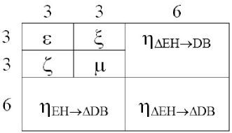
Figure 5: The block structure of the extended material parameter matrix, with the numbers of rows/columns in hte blocks shown.

The leading $6\times 6$ block contains the standard electromagnetic parameters: the $\epsilon$ and $\mu$ tensors as well as magnetoelectric coupling parameters $\xi$ and $\zeta$ (also in general tensorial). The remaining blocks are novel; they quantify spatial dispersion. In particular, the $\eta_{\mathrm{\Delta}\mathrm{EH}\rightarrow\mathrm{DB}}$ block, as the notation suggests, characterizes the dependence of fields $\mathbf{D}$ and $\mathbf{B}$ on the variations of $\mathbf{E}$ and $\mathbf{H}$ within the cell rather than on their mean values.

5 Application Examples

5.1 Tutorial: Homogeneous Cell Revisited

This case, the simplest but still nontrivial, doubles as a tutorial example where construction of all approximating functions and matrices can be demonstrated in closed form. In [2, 31], it was shown that the exact result $\epsilon_{\mathrm{eff}}=\epsilon$, $\mu_{\mathrm{eff}}=1$ can be obtained for a homogeneous cell with a permittivity $\epsilon$ and permeability $\mu=1$ if plane waves are used as the basis modes. However, one cannot expect such a perfect result in general, due to approximations involved in any homogenization procedure. It is instructive to see how the proposed methodology works for the homogeneous cell if Whitney-like values for the basis waves on the cell boundary are used instead of plane/Bloch waves.

To make the demonstration most transparent, consider the 2D case, $H$-mode ($p$-mode), governed by the wave equation

$$\nabla^{2}h\,+\,k^{2}h~{}=~{}0$$

where in a homogeneous cell $k$ = const. In this example, as in the section on interpolating functions, it is convenient to normalize the cell size $a$ to unity, to shorten the notation. Then in the square lattice cell $\mathrm{\Omega}=[0,1]^{2}$, the four approximating functions $\psi^{(h)}_{1-4}$ for the $h$ field are chosen to satisfy the wave equation and Whitney-like conditions on the cell boundary $\partial\mathrm{\Omega}$

$$\psi^{(h)}_{1}(\partial\mathrm{\Omega})=xy;~{}~{}\psi^{(h)}_{2}(\partial\mathrm{\Omega})=(1-x)y;$$

$$\psi^{(h)}_{3}(\partial\mathrm{\Omega})=x(1-y);~{}~{}\psi^{(h)}_{4}(\partial\mathrm{\Omega})=(1-x)(1-y)$$ (15)

Inside the cell, these functions can be found using a variety of semi-analytical or numerical methods. For example, separation of variables leads to the following expression for $\psi^{(h)}_{1}$ ($\psi^{(h)}_{2-4}$ being completely similar):

$$\psi^{(h)}_{1}\,=\,xy\,-\,k^{2}\sum\nolimits_{n_{x,y}=-\infty}^{\infty}c_{n_{x},n_{y}}\sin(n_{x}\kappa x)\sin(n_{y}\kappa y),$$

where $\kappa=\pi/a$ in general and $\kappa=\pi$ for the unit cell; $c_{n_{x},n_{y}}=4f_{n_{x},n_{y}}/(k^{2}-\kappa^{2}(n_{x}^{2}n_{y}^{2}))$, $f_{n_{x},n_{y}}=(\sin\pi n_{x}-\pi n_{x}\cos\pi n_{x})(\sin\pi n_{y}-\pi n_{y}\cos\pi n_{y})/(\pi^{4}n_{x}^{2}n_{y}^{2})$.

With the approximating functions $\psi^{(h)}_{1-4}$ for the $h$ field available, the respective basis waves $\psi^{(e)}_{1-4}$ for the $e$ field are immediately found by differentiation, from Maxwell’s equations.

To find the effective parameter matrix $\eta$ from (9), we need to populate the matrices $\Psi^{EH}$ and $\Psi^{DB}$. The first one contains the edge-averaged $e$ and $h$ fields of the basis waves. For the 2D case, $p$-mode, the latter degenerate simply to the values of $h$ at the nodes of the lattice cell. (For the $s$-mode, the circulations of the $e$ field degenerate to the nodal values of the field.)

Matrix $\Psi^{DB}$ contains the face-averaged $\mathbf{d}$ and $\mathbf{b}$ fields. For the 2D case, $p$-mode, “face-averaging” of the $\mathbf{d}$ field turns into edge-averaging of its component normal to the respective edge, and “face-averaging” of the $\mathbf{b}$ field turns into averaging over the whole lattice cell. (For the $s$-mode, the manipulation of $\mathbf{d}$ and $\mathbf{b}$ in this procedure would be reversed.)

Let us illustrate this calculation for the first basis mode $\psi^{(h)}_{1},\psi^{(e)}_{1}$. The four edge-averaged values of the $\mathbf{e}$ field are

$$e_{x1}=\int_{x=0}^{1}\psi^{(e)}_{1x}(x,0)dx;~{}~{}~{}e_{x3}=\int_{x=0}^{1}\psi^{(e)}_{1x}(x,1)dx;$$

$$e_{y2}=\int_{y=0}^{1}\psi^{(e)}_{1y}(1,y)dy;~{}~{}~{}e_{y4}=\int_{y=0}^{1}\psi^{(e)}_{1y}(0,y)dy$$

The edges are numbered counterclockwise, starting from the edge $[0,1]$ on the $x$ axis. The first column of $\Psi^{EH}$ corresponds to the first basis mode, and the first two entries of that column are

$$\Psi^{EH}_{11}\equiv(e_{x1}+e_{x3})/2;~{}~{}\Psi^{EH}_{21}\equiv(e_{y2}+e_{y4})/2$$

The first entry is the mean value of the $x$-components of the electric field along edges 1 and 3 (the “horizontal” edges) of the cell; the second entry is the mean value of the $y$-components over the “vertical” edges 2 and 4.

The third entry of this first column is just the average $h$ field at the nodes of the cell:

$$\Psi^{EH}_{31}~{}=~{}(h_{1}+h_{2}+h_{3}+h_{4})/4$$

where $h_{1}=\psi^{(h)}_{1}(0,0)$, $h_{2}=\psi^{(h)}_{1}(1,0)$, $h_{3}=\psi^{(h)}_{1}(1,1)$, $h_{4}=\psi^{(h)}_{1}(0,1)$.

The fourth and final entry in the first column of $\Psi^{EH}$ is

$$(ka)^{2}\Psi^{EH}_{41}=h_{1}+h_{3}-h_{2}-h_{4}=0+1-0-0=1$$

Computing the first column of the EH matrix as defined above (with a separation-of-variables expansion of the first basis mode), one obtains $(0.5\mathrm{i}(\epsilon ka)^{-1},-0.5\mathrm{i}(\epsilon ka)^{-1},0.25,1/(ka)^{2})^{T}$, with $a=1$ for the unit cell. The remaining three columns of this matrix correspond to the other three basis waves and differ from the first one only through cyclic permutation and some sign changes.

Consider now the first column of the DB matrix $\Psi^{DB}$. This column corresponds to the first basis mode, and other columns are completely analogous. First, we need the fluxes of the basis wave through the four edges of the cell. For the bottom edge (edge #1)

$$d_{y1}=a^{-1}\,\epsilon\int_{x=0}^{a}\psi^{(e)}_{1y}(x,0)dx=1/(\mathrm{i}\omega a)(h_{2}-h_{1})$$

(with $a=1$ if the cell is scaled to unit size); $d_{x2},d_{x4}$, and $d_{y3}$ are expressed analogously. For the Whitney-type basis functions with bilinear boundary conditions (15), these expressions are in fact quite simple. For the first basis wave, $h_{3}=1$ and $h_{1}=h_{2}=h_{4}=0$.

The first entry of the first column is the mean value of the $x$-component of the $\mathbf{d}$ field along edges 2 and 4 (the “vertical” edges) of the cell, and the second entry is the mean value of the $y$ component along the horizontal edges:

$$\Psi^{DB}_{11}\equiv\langle d_{x}\rangle\equiv(d_{x2}+d_{x4})/2$$

$$\Psi^{DB}_{21}\equiv\langle d_{y}\rangle\equiv(d_{y1}+d_{y3})/2$$

The third entry is the average $B$ field over the cell:

$$\Psi^{DB}_{31}~{}=~{}\int_{x=0}^{a}\int_{y=0}^{a}\psi^{(b)}(x,y)dxdy$$

There are somewhat different ways to define the fourth entry; for example,

$$ka\Psi^{DB}_{31}~{}=~{}\mathrm{\Delta}_{x}\langle d_{x}\rangle-\mathrm{\Delta}_{y}\langle d_{y}\rangle$$

The actual calculation of the first column yields $(0.5\mathrm{i}(ka)^{-1},-0.5\mathrm{i}(ka)^{-1},0.25,0)^{T}$, the other three columns being very similar.

Solving for the $4\times 4$ material parameter matrix $\eta$, one verifies that, as expected, its only nonzero entries are $\epsilon_{xx}=\epsilon_{yy}$ and $\mu$. The “spatial dispersion block” – in this case, a single column #4 of the matrix – is zero, indicating the absence of “spatial dispersion” for a homogeneous cell, as also expected. The effective parameters are not exactly equal to one but rather $\epsilon_{xx}=\epsilon_{yy}\approx 1+5\cdot 10^{-5}(ka)^{-1}$, $\mu\approx 1+3.5\cdot 10^{-5}(ka)^{-1}$. The small deviation from unity is a result of the approximations involved – namely, of the free-space fields in the cell by spatially bilinear basis modes.

5.2 Inclusions with Interior Resonances

This example involves high-permittivity inclusions with strong resonance effects and elements of spatial dispersion. The setup and parameters are very similar to the ones in [36, 37], where a special asymptotic method was developed to handle resonances and additional adjustable parameters [37] were needed. The methodology of the present paper handles this case with relative ease and without any additional assumptions or parameters.

The lattice cell contains a high-permittivity ($\epsilon_{\mathrm{incl}}=200+5\mathrm{i}$) cylindrical inclusion; its radius relative to the cell size is $r/a=0.25$; the vacuum wavelength $\lambda/a$ varies from 5 to 12. It is interesting to consider the $H$-mode ($p$-mode) where the electric field cuts across the cylinders and strong resonances can be induced.

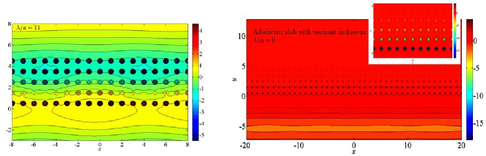
Figure 6: Re$(H)$ in the vicinity of a slab with resonant inclusions; $p$-mode. Radius of the inclusions relative to the cell size $r/a=0.25$; their permittivity $\epsilon_{\mathrm{incl}}=200+5\mathrm{i}$ (as in [37]). Left: pass band, $\lambda/a=11$; right: bandgap, $\lambda/a=9$; inset: zoom-in on a few cells.

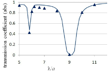
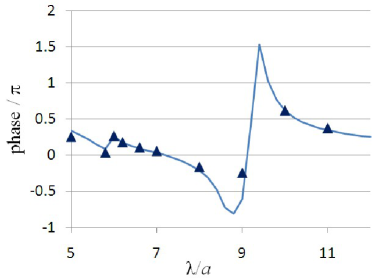
Figure 7: Transmission coefficient (with respect to $H$) of a five-layer slab as a function of the vacuum wavelength (top: absolute value, bottom: phase). $r/a=0.25$; $\epsilon_{\mathrm{incl}}=200+5\mathrm{i}$. Triangles: direct finite difference simulation [34]; lines: slab with effective parameters. Normal incidence.

The effective medium theory developed here agrees very well with “brute force” finite difference simulations where all inclusions are represented directly. As in [2], propagation of waves through a homogeneous “effective parameter” slab is compared with the numerical simulation of this propagation through the actual metamaterial; high-order finite difference “FLAME” schemes ([33, 34, 32] were used for the numerical simulation. For illustration, Fig. 6 shows the color plots of the real part of the magnetic field for normal incidence in the pass band, $\lambda/a=11$, and in the bandgap, $\lambda/a=9$.

Fig. 7 demonstrates that the transmission coefficient for the slab with effective parameters is very close, both in the absolute value and phase, to the “true” coefficient from the accurate finite difference simulation.

The effective parameters plotted in Fig. 8 are completely physical; they do exhibit physical resonances but no “antiresonances”. A fairly weak electric resonance is observed near $\lambda/a\sim 5.5$ and a strong magnetic resonance – around $\lambda/a\sim 9$. As should be expected by symmetry considerations, the magnetoelectric coupling is in this example zero (numerically, it is at the roundoff error level).

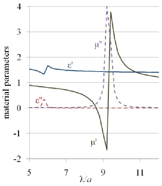
Figure 8: Effective parameters of the metamaterial with resonant inclusions at the center of the lattice cell.

The entries $\eta_{14}$, $\eta_{24}$ and $\eta_{34}$ of the parameter matrix – measures of nonlocality – are in this case zero, too. However, this is no longer so if the inclusions are shifted to, for instance, $(x_{0},y_{0})=(0.1a,0.1a)$ relative to the center of the cell. Parameters $\epsilon_{\mathrm{eff}}$ and $\mu_{\mathrm{eff}}$ are almost unaffected by this shift (third- or fourth-digit differences). However, $\eta_{14}=\eta_{24}$ and $\eta_{34}$ now have absolute values on the order of 0.05 or less (Fig. 9), and going down to zero in the long-wavelength limit, as expected.

This weakly nonlocal response is consistent with physical intuition and is clearly due to the appreciable size of the cell relative to the vacuum wavelength and especially to the wavelength in the inclusions. Why, though, does not the nonlocality manifest itself when the inclusions are located at the center of the cell? Nonlocality reflects the fact that the behavior of the fields within the cell is too complex to be described (at a given level of approximation) just by the field averages; more information is needed and comes in the form of field variations. However, when the cell is symmetric, fewer parameters may suffice to describe the field (this is akin to, say, the permittivity tensor degenerating to a single scalar value in the symmetric case); hence one can make do without any additional nonlocality parameters unless a much higher level of approximation is desired.

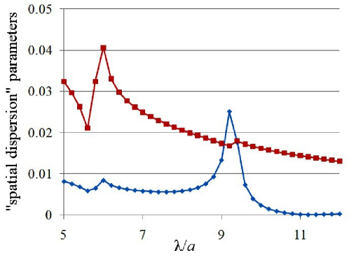
Figure 9: The absolute values of the “spatial dispersion” parameters $\eta_{14}=\eta_{24}$ (squares) and $\eta_{34}$ of the metamaterial with resonant inclusions. Shifted inclusions centered at $x_{0}=y_{0}=0.1a$ relative to the cell center.

6 Conclusion

The proposed homogenization theory stems from a small number of fundamental principles – most importantly, that the coarse-grained fields must satisfy Maxwell’s equations and boundary conditions and that material parameters are, by definition, linear relations between the coarse-grained fields. Consequently, the $\mathbf{E}$ and $\mathbf{H}$ fields are produced by an interpolation that preserves tangential continuity (see Section 3 and [2]), while for $\mathbf{D}$ and $\mathbf{B}$ the normal continuity is maintained.

The number of degrees of freedom (d.o.f.) for the coarse-grained fields depends on the specific interpolation procedures chosen. (For example, the most natural choice for a parallelepipedal lattice cell results in 24 d.o.f. for the $(\mathbf{E},\mathbf{H})$ pair and 12 d.o.f. for the $(\mathbf{D},\mathbf{B})$ pair.) Technically, therefore, the generalized “material parameter” can be represented by a large matrix that encodes a substantial amount of information about the behavior of the fields in the cell. This parameter matrix acquires a clear physical meaning upon transformation to a “canonical” basis where the coarse-grained fields are expressed as their average values plus variations. In this canonical representation, the matrix has a leading $6\times 6$ diagonal block that represents the standard effective parameters: the permittivity, permeability and magnetoelectric tensors. The remaining matrix blocks – linking the average values of the coarse-grained fields to their variations over the cell – may serve as a quantitative measure of spatial dispersion.

The new theory is a substantial extension of the methodology put forward in [2]. The overall structure of the procedure (cf. Fig. 1) and its core – two different types of interpolating functions for different fields – remain the same. However, the linear relations between the coarse-grained fields are now established and handled differently, allowing one to evaluate not only the traditional electromagnetic parameters but also some quantitative measures of spatial dispersion as described above. Furthermore, this paper breaks away from the exclusive reliance on Bloch waves as approximating modes for the field. While propagating Bloch modes are indispensable in the analysis of periodic structures, their value for nonperiodic media and especially for evanescent waves is limited; in addition, Bloch modes are expensive to compute. One possible alternative is low-order polynomial approximation of the fields on lattice cell boundaries.

The proposed theory does not involve any heuristic assumptions or artificial averaging rules. The effective parameters are defined directly via field analysis in the lattice cell, in contrast with methods where these parameters are obtained from reflection/transmission data or other indirect considerations. Nontrivial magnetic behavior, if present, follows logically from the method. The necessary approximations are clearly identifiable and measurable. Examples include a tutorial on the method and an analysis of a resonant structure with high-permittivity inclusions.

References

- [1]
- [2] Igor Tsukerman. Effective parameters of metamaterials: a rigorous homogenization theory via Whitney interpolation. J Opt Soc Am B, 28:577–586 (2011).
- [3] D. R. Smith, S. Schultz, P. Markoš, and C. M. Soukoulis, Determination of effective permittivity and permeability of metamaterials from reflection and transmission coefficients, Phys. Rev. B 65, 195104 (2002).
- [4] X. Chen, B.-I. Wu, J. A. Kong, and T. M. Grzegorczyk, Retrieval of the effective constitutive parameters of bianisotropic metamaterials, Phys. Rev. E 71, 046610 (2005).
- [5] Z. Li, K. Aydin, and E. Ozbay, Determination of the effective constitutive parameters of bianisotropic metamaterials from reflection and transmission coefficients, Phys. Rev. E 79, 026610 (2009).
- [6] D.-H. Kwon, D. H. Werner, A. V. Kildishev, and V. M. Shalaev, Material parameter retrieval procedure for general bi-isotropic metamaterials and its application to optical chiral negative-index metamaterial design, Opt. Express 16, 11822 (2008).
- [7] X. Chen, T. M. Grzegorczyk, B.-I. Wu, J. Pacheco, and J. A. Kong, Robust method to retrieve the constitutive effective parameters of metamaterials, Phys. Rev. E 70, 016608 (2004).
- [8] A. K. Sarychev and V. M. Shalaev. Electrodynamics of Metamaterials. (World Scientific, Singapore, 2007).
- [9] C. R. Simovski. On material parameters of metamaterials (review). Opt & Spectr, 107:726–753 (2009).
- [10] C. R. Simovski and S. A. Tretyakov. On effective electromagnetic parameters of artificial nanostructured magnetic materials. Photonics & Nanostr, 8:254–263 (2010).
- [11] C. Scheiber, A. Schultschik, O. Bíró, R.Dyczij-Edlinger. A model order reduction method for efficient band structure calculations of photonic crystals, IEEE Trans Magn, 47(5), 1534–1537 (2011).
- [12] I. Babuška and J.M. Melenk. The partition of unity method. Int. J. for Numer. Meth. in Eng., 40(4):727–758 (1997).
- [13] A. Plaks, I. Tsukerman, G. Friedman, and B. Yellen. Generalized Finite Element Method for magnetized nanoparticles. IEEE Trans. Magn., 39(3):1436–1439 (2003).
- [14] Ivo Babuška and Robert Lipton. Optimal local approximation spaces for generalized finite element methods with application to multiscale problems. Multiscale Modeling and Simulation, SIAM 9:373-406 (2011).
- [15] R. Hiptmair, A. Moiola and I. Perugia. Error analysis of Trefftz-discontinuous Galerkin methods for the time-harmonic Maxwell equations, Preprint IMATI-CNR Pavia, 5PV11/3/0, http://www-dimat.unipv.it/perugia/PREPRINTS/TDGM.pdf (2011).
- [16] Gene H. Golub and Charles F. Van Loan. Matrix Computations. (The Johns Hopkins University Press: Baltimore, MD, 1996).
- [17] James W. Demmel. Applied Numerical Linear Algebra. (SIAM; 1997).
- [18] Chris Fietz and Gennady Shvets. Homogenization theory for simple metamaterials modeled as one-dimensional arrays of thin polarizable sheets. Phys Rev B 82, 205128 (2010).
- [19] M. G. Silveirinha. Metamaterial homogenization approach with application to the characterization of microstructured composites with negative parameters. Phys Rev B, 75(11):115104 (2007).
- [20] Chris Fietz and Gennady Shvets. Current-driven metamaterial homogenization. Physica B: Cond Mat 405(14), 2930–2934 (2010).
- [21] David R. Smith and John B. Pendry. Homogenization of metamaterials by field averaging. J. Opt Soc. Am B, 23(3):391–403 (2006).
- [22] H. Whitney. Geometric Integration Theory. (Princeton, NJ: Princeton Univ. Press, 1957).
- [23] Alain Bossavit. Computational Electromagnetism: Variational Formulations, Complementarity, Edge Elements. (San Diego: Academic Press, 1998).
- [24] L.D. Landau and E.M. Lifshitz. Electrodynamics of Continuous Media. (Oxford; New York: Pergamon, 1984).
- [25] Vadim A. Markel. Private communication, 2010–2011.
- [26] Vadim A. Markel. On the current-driven model in the classical electrodynamics of continuous media. J Phys: Cond Mat, 22(48):485401 (2010).
- [27] Igor Tsukerman. Negative refraction and the minimum lattice cell size. J. Opt. Soc. Am. B, 25:927–936 (2008).
- [28] A. P. Vinogradov. On the form of constitutive equations in electrodynamics. Phys. Usp., 45:331 -338 (2002).
- [29] Carl de Boor. Divided differences. Surv. Approx. Theory 1:46–69 (2005).
- [30] V. M. Agranovich and V. L. Ginzburg. Crystal Optics with Spatial Dispersion, and Excitons. (Berlin; New York: Springer-Verlag (2nd ed.), 1984).
- [31] Anders Pors, Igor Tsukerman, Sergey I. Bozhevolnyi. Effective constitutive parameters of plasmonic metamaterials: homogenization by dual field interpolation. Phys Rev E, accepted. arXiv:1104.2972 (2011).
- [32] I. Tsukerman and F. Čajko. Photonic band structure computation using FLAME. IEEE Trans Magn, 44(6):1382–1385 (2008).
- [33] I. Tsukerman. A class of difference schemes with flexible local approximation. J. Comput. Phys., 211(2):659–699 (2006).
- [34] Igor Tsukerman. Computational Methods for Nanoscale Applications: Particles, Plasmons and Waves. (Springer, 2007).
- [35] Jonathon Shlens. A tutorial on principal component analysis, http://www.snl.salk.edu/shlens/pca.pdf (2009).
- [36] D. Felbacq, G. Bouchitté. Theory of mesoscopic magnetism in photonic crystals. Phys Rev Lett, 94:183902 (2005).
- [37] D. Felbacq, B. Guizal, G. Bouchitté, C. Bourel. Resonant homogenization of a dielectric metamaterial. Microwave and Opt Tech Lett, 51:2695–2701 (2009).