Exact solutions of Brans-Dicke wormholes in the presence of matter

Abstract

A fundamental ingredient in wormhole physics is the presence of exotic matter, which involves the violation of the null energy condition. Although a plethora of wormhole solutions have been explored in the literature, it is useful to find geometries that minimize the usage of exotic matter. In this work, we find exact wormhole solutions in Brans-Dicke theory where the normal matter threading the wormhole satisfies the null energy condition throughout the geometry. Thus, the latter implies that it is the effective stress-energy tensor containing the scalar field, that plays the role of exotic matter, that is responsible for sustaining the wormhole geometry. More specifically, we consider a zero redshift function and a particular choice for the scalar field and determine the remaining quantities, namely, the stress-energy tensor components and the shape function. The solution found is not asymptotically flat, so that this interior wormhole spacetime needs to be matched to an exterior vacuum solution.

I Introduction

Wormholes are hypothetical short-cuts in spacetime and, in classical general relativity, are supported by exotic matter Morris . The latter involves a stress-energy tensor $T_{\mu\nu}$ that violates the null energy condition (NEC), i.e., $T_{\mu\nu}k^{\mu}k^{\nu}<0$, where $k^{\mu}$ is a null vector. In fact, wormholes violate all the pointwise energy conditions and the averaged energy conditions. The latter averaged energy conditions are somewhat weaker than the pointwise energy conditions, as they permit localized violations of the energy conditions, as long on average the energy conditions hold when integrated along timelike or null geodesics Tipler . In this context, although a plethora of wormhole solutions have been explored in the literature whsolutions , it is useful to find geometries that minimize the usage of exotic matter and this has been obtained in several manners. In Visser:2003yf a suitable measure for quantifying this notion was developed, and it was demonstrated that spacetime geometries containing traversable wormholes supported by arbitrarily small quantities of “exotic matter” can indeed be constructed. Another way to minimize the usage of exotic matter is to construct thin-shell wormholes using the cut-and-paste procedure, where the exotic matter is concentrated at the throat thinshell . In the context of modified theories of gravity, it has also been shown that the stress-energy tensor can be imposed to satisfy the NEC, and it is the higher order curvature terms, interpreted as a gravitational fluid, that sustain these non-standard wormhole geometries, fundamentally different from their counterparts in general relativity modgrav .

In this context, we find exact wormhole solutions in Brans-Dicke theory where the normal matter threading the wormhole satisfies the NEC, and it is the effective stress-energy tensor containing the scalar field that is responsible for the null energy condition violation. The analysis in this paper builds on previous work Anchordoqui:1996jh . In the latter work, the authors consider an equation of state give by $p_{r}+p_{t}=\epsilon\rho$, where $p_{r}$, $p_{t}$ and $\rho$ are the radial pressure, tangential pressure and the energy density, respectively. The authors then deduce the form of the scalar field and outline rather general conditions of the parameter space in which the Brans- Dicke field may play the role of exotic matter, implying that it might be possible to build a wormholelike spacetime with the presence of ordinary matter at the throat. We generalize the latter work, showing that it is possible to construct wormhole geometries with normal matter satisfying the NEC throughout the spacetime. These works, in turn, generalize the vacuum Brans-Dicke wormholes that have been analysed in the literature Agnese:1995kd ; Anchordoqui:1996jh ; Lobo:2010sb ; Nandi:1997en ; Nandietal ; Nandietal2 . In particular, specific solutions were constructed showing that static wormhole solutions in vacuum Brans-Dicke theory only exist in a narrow interval of the coupling parameter Nandi:1997en , namely, $-3/2<w<-4/3$. It should be emphasized that this range is obtained for vacuum solutions and for a specific choice of an integration constant of the field equations given by $C(w)=-1/(w+2)$. The latter relationship was derived on the basis of a post-Newtonian weak field approximation, and there is no reason for it to hold in the presence of compact objects with strong gravitational fields. In fact, the choice given by the above form of $C(w)$ is a tentative example and reflects how crucially the wormhole range for $w$ depends on the form of $C(w)$. Indeed, specific examples for $C(w)$ were given in Lobo:2010sb that lie outside the range $-3/2<w<-4/3$.

This paper is organised in the following manner: In Section II, we write the field equations and the specific constraints imposed by the violations of the null energy condition. In Section III, we consider a specific solution by considering a zero redshift function and a particular choice for the scalar field. Finally, in Section IV, we conclude.

II Field equations

The field equations of Brans-Dicke theory are given by bruck

$$R_{\mu\nu} = \frac{8\pi}{\Phi}\left(T_{\mu\nu}-\frac{\omega+1}{2\omega+3}\;T\>g_{\mu\nu}\right)+\omega\>\frac{\Phi_{;\mu}\Phi_{;\nu}}{\Phi^{2}}+\frac{\Phi_{;\mu;\nu}}{\Phi}\,,$$ (1)

$$\Phi^{;\mu}_{\;;\mu} = \frac{8\pi}{2\omega+3}\;T\,,$$ (2)

where $T$ is the trace of the stress-energy tensor, $\Phi$ is the scalar field, $\omega$ the Brans- Dicke parameter, $R_{\mu\nu}$ the Ricci tensor and $g_{\mu\nu}$ the metric tensor.

Using the the line element written in Schwarzschild coordinates

$$ds^{2}=-e^{2\psi}dt^{2}+e^{2\lambda}dr^{2}+r^{2}(d\theta^{2}+\sin^{2}\theta d\phi^{2})\,,$$ (3)

the field equations take the following form

$$-\psi^{\prime\prime}-(\psi^{\prime})^{2}+\lambda^{\prime}\psi^{\prime}+2\frac{\lambda^{\prime}}{r} = \frac{8\pi}{\Phi}\left[p_{r}-\frac{\omega+1}{2\omega+3}\;T\right]e^{2\lambda}+(\omega+1)(\ln\Phi)^{\prime 2}+(\ln\Phi)^{\prime\prime}-\lambda^{\prime}(\ln\Phi)^{\prime}\,,$$ (4)

$$1-re^{-2\lambda}\left[\psi^{\prime}-\lambda^{\prime}+\frac{1}{r}\right] = \frac{8\pi}{\Phi}\left[p_{t}-\frac{\omega+1}{2\omega+3}\;T\right]r^{2}+re^{-2\lambda}(\ln\Phi)^{\prime}\,,$$ (5)

$$e^{2(\psi-\lambda)}\left[\psi^{\prime\prime}+(\psi^{\prime})^{2}-\lambda^{\prime}\psi^{\prime}+2\frac{\psi^{\prime}}{r}\right] = \frac{8\pi}{\Phi}\left[\rho+\frac{\omega+1}{2\omega+3}\;T\right]e^{2\psi}-\psi^{\prime}e^{2(\psi-\lambda)}(\ln\Phi)^{\prime}\,,$$ (6)

$$\Phi^{\prime\prime}-\Phi^{\prime}\left(\lambda^{\prime}-\psi^{\prime}-\frac{2}{r}\right) = \frac{8\pi}{2\omega+3}\;T\;e^{2\lambda}\,,$$ (7)

respectively, where the prime denotes a derivative with respect to the radial coordinate. $\rho(r)$ is the energy density, $p_{r}(r)$ is the radial pressure, and $p_{t}(r)$ is the tangential pressure. The Bianchi identity, $G^{\mu\nu}{}_{;\nu}=0$, implies that for a static spherically symmetric anisotropic fluid, we have

$$p_{r}^{\prime}=-(\rho+p_{r})\psi^{\prime}+\frac{2(-p_{r}+p_{t})}{r}\,.$$ (8)

One now has at hand four equations, namely, the field Eqs. (4)-(7), with six unknown functions of $r$, i.e., $\rho(r)$, $p_{r}(r)$, $p_{t}(r)$, $\psi(r)$, $\lambda(r)$ and $\Phi(r)$. To construct specific solutions, one may adopt several approaches, and in this work we mainly use the strategy of considering restricted choices for the redshift function and for the scalar field $\Phi(r)$, in order to obtain solutions with the properties and characteristics of wormholes.

A fundamental property of wormhole physics is the violation of the null energy condition at the throat Morris . In this context, it is useful to write the field equation in the form $G_{\mu\nu}=8\pi T_{\mu\nu}^{\textrm{Eff}}$ where $T_{\mu\nu}^{\textrm{Eff}}$ is given by

$$T_{\mu\nu}^{Eff}=\frac{T_{\mu\nu}}{\Phi}+\frac{1}{8\pi}\left[\frac{\omega}{\Phi^{2}}(\Phi_{;\mu}\Phi_{;\nu}-\frac{1}{2}g_{\mu\nu}\Phi^{;\alpha}\Phi_{;\alpha})+\frac{1}{\Phi}(\Phi_{;\mu\nu}-g_{\mu\nu}\Phi^{;\alpha}_{;\alpha})\right]\,.$$ (9)

The violation of the NEC states that $T^{\textrm{Eff}}_{\mu\nu}k^{\mu}k^{\nu}<0$, where $k$ is any null vector, and imposes the following constraint

$$\left\{[8\pi(\rho+p_{r})+e^{-2\lambda}\left[\Phi^{\prime\prime}-\Phi^{\prime}(\lambda^{\prime}+\Psi^{\prime})+\frac{\omega}{\Phi}(\Phi^{\prime})^{2}\right]\right\}\Big{|}_{r_{0}}<0\,.$$ (10)

In this work, we also impose that the normal matter threading the wormhole satisfies the NEC, $T_{\mu\nu}k^{\mu}k^{\nu}>0$. At the throat this states that $(\rho+p_{r})|_{r_{0}}>0$. Thus, it is useful to rewrite the components $\rho(r)$, $p_{r}(r)$ and $p_{t}(r)$, as a function of the metric functions $\psi(r)$ and $\lambda(r)$ and the scalar field $\Phi(r)$. Note that one may simply substitute the factor $T/(2\omega+3)$ of Eq. (7) into Eqs. (4)-(6), which yield the following relationships

$$\rho = \frac{e^{-2\lambda}\Phi}{8\pi}\left\{\psi^{\prime\prime}+\psi^{\prime 2}+\psi^{\prime}\left[-\lambda^{\prime}-\omega(\ln\Phi)^{\prime}+\frac{2}{r}\right]-(\omega+1)\left[(\ln\Phi)^{\prime\prime}+(\ln\Phi)^{\prime}-(\ln\Phi)^{\prime}\left(\lambda^{\prime}-\frac{2}{r}\right)\right]\right\},$$ (11)

$$p_{r} = \frac{e^{-2\lambda}\Phi}{8\pi}\left\{-\psi^{\prime\prime}-\psi^{\prime 2}+\psi^{\prime}[\lambda^{\prime}+(\omega+1)(\ln\Phi)^{\prime}]+\omega(\ln\Phi)^{\prime\prime}+(\ln\Phi)^{\prime}(\omega\lambda^{\prime}+\frac{2}{r}(\omega+1))\right\},$$ (12)

$$p_{t} = \frac{\Phi}{8\pi r^{2}}\left\{1-re^{-2\lambda}(\psi^{\prime}-\lambda^{\prime}+(\ln\Phi)^{\prime}+\frac{1}{r})+(\omega+1)r^{2}\left[(\ln\Phi)^{\prime\prime}+(\ln\Phi)^{\prime}2-(\ln\Phi)^{\prime}(\lambda^{\prime}-\psi^{\prime}-\frac{2}{r})\right]\right\}\,,$$ (13)

respectively. These equations will be explored further below.

III Exact solution: Zero redshift function

In this section, we consider the wormhole metric given in the more familiar spherically symmetric and static form Morris

$$ds^{2}=-e^{2\psi(r)}\,dt^{2}+\frac{dr^{2}}{1-b(r)/r}+r^{2}\,(d\theta^{2}+\sin^{2}{\theta}\,d\phi^{2})\,.$$ (14)

Comparing with the metric (3), this corresponds to the following identification

$$\lambda(r)=-\frac{1}{2}\ln\left(1-\frac{b(r)}{r}\right)\,,$$ (15)

where $\psi(r)$ and $b(r)$ are arbitrary functions of the radial coordinate, $r$. Following the conventions used in Morris , $\psi(r)$ is denoted as the redshift function, for it is related to the gravitational redshift; $b(r)$ is called the shape function, because as can be shown by embedding diagrams, it determines the shape of the wormhole Morris . A fundamental property of a wormhole is that a flaring out condition of the throat, given by $(b-b^{\prime}r)/b^{2}>0$, is imposed Morris , and at the throat $b(r_{0})=r=r_{0}$, the condition $b^{\prime}(r_{0})<1$ is imposed to have wormhole solutions. This latter condition will be explored below. Note that the condition $1-b/r>0$ is also imposed. It is possible to construct asymptotically flat spacetimes, in which $b(r)/r\rightarrow 0$ and $\psi\rightarrow 0$ as $r\rightarrow\infty$. However, one may also construct solutions by matching the interior solution to an exterior vacuum spacetime, at a junction interface, much in the spirit of matching . The latter case is applied in this work, as will be shown below.

For simplicity, we consider the specific case of a zero redshift function, $\psi=0$, so that Eq. (6) provides the following relationship

$$p_{t}=-\frac{1}{2}\left[p_{r}+\left(\frac{\omega+2}{\omega+1}\right)\rho\right],$$ (16)

and (8) yields

$$p_{r}^{\prime}=-\frac{1}{r}\left[3p_{r}+\left(\frac{\omega+2}{\omega+1}\right)\rho\right].$$ (17)

In addition to the zero redshift function, we consider the ansatz $\Phi=\Phi_{0}\left(\frac{r_{0}}{r}\right)^{\alpha},$ with $\Phi_{0}>0$ and $\alpha>0$, so that the field equations can be written in the following manner

$$\left(1-\frac{\alpha}{2}\right)b^{\prime}+\left[(\omega+1)\alpha^{2}+\frac{3\alpha}{2}-1\right]\frac{b}{r}-(\omega+1)\alpha^{2}-\alpha = \frac{8\pi r^{2}}{\Phi_{0}}(\rho+p_{r})\left(\frac{r_{0}}{r}\right)^{-\alpha},$$ (18)

$$b^{\prime}+\frac{b}{r}(1-2\alpha)+2\alpha = \frac{8\pi r^{2}}{\Phi_{0}}\left[\left(\frac{\omega}{\omega+1}\right)\rho-p_{r}\right]\left(\frac{r_{0}}{r}\right)^{-\alpha},$$ (19)

$$b^{\prime}+(1-2\alpha)\frac{b}{r}+2(\alpha-1) = -\frac{16\pi\rho r^{2}}{(\omega+1)\alpha\Phi_{0}}\left(\frac{r_{0}}{r}\right)^{-\alpha}.$$ (20)

The solution of this system is given by the following stress-energy components

$$\rho(r) = \frac{1}{4\pi r_{0}^{2}}\left[\frac{\alpha(\omega+1)c_{1}}{\omega\alpha+2}\left(\frac{r_{0}}{r}\right)^{\frac{2(\alpha+2\omega\alpha+3)}{\omega\alpha+2}}+\frac{(\alpha-1)\alpha\Phi_{0}(\omega+1)}{(\omega\alpha^{2}-2\omega\alpha-2)}\left(\frac{r_{0}}{r}\right)^{\alpha+2}\right],$$ (21)

$$p_{r}(r) = \frac{1}{4\pi r_{0}^{2}}\left[c_{1}\left(\frac{r_{0}}{r}\right)^{\frac{2(\alpha+2\omega\alpha+3)}{\omega\alpha+2}}+\frac{(\omega+2)\alpha\Phi_{0}}{(\omega\alpha^{2}-2\omega\alpha-2)}\left(\frac{r_{0}}{r}\right)^{\alpha+2}\right],$$ (22)

$$p_{t}(r) = -\frac{1}{4\pi r_{0}^{2}}\left[\frac{c_{1}(\omega\alpha+\alpha+1)}{\omega\alpha+2}\left(\frac{r_{0}}{r}\right)^{\frac{2(\alpha+2\omega\alpha+3)}{\omega\alpha+2}}+\frac{\alpha^{2}\Phi_{0}(\omega+2)}{2(\omega\alpha^{2}-2\omega\alpha-2)}\left(\frac{r_{0}}{r}\right)^{\alpha+2}\right]\,,$$ (23)

respectively, and the shape function is provided by

$$b(r)=r_{0}\left[\frac{\omega\alpha(\alpha-2)}{\omega\alpha^{2}-2\omega\alpha-2}\left(\frac{r}{r_{0}}\right)+\frac{4c_{1}}{\Phi_{0}(\omega\alpha^{2}+4\alpha-2)}\left(\frac{r_{0}}{r}\right)^{\frac{\alpha\omega(1-\alpha)}{\omega\alpha+2}}+c_{2}\left(\frac{r_{0}}{r}\right)^{-1+2\alpha}\right],$$ (24)

where $c_{1}$ and $c_{2}$ are constants of integration. $c_{1}$ is given by

$$c_{1}=\frac{(\omega\alpha+2)[4\pi r_{0}^{2}(\omega\alpha^{2}-2\omega\alpha-2)(\rho_{0}+p_{r}(r_{0}))-(\omega\alpha^{2}+\alpha^{2}+\alpha)\Phi_{0}]}{(\omega\alpha^{2}-2\omega\alpha-2)(\alpha+2\omega\alpha+2)}.$$ (25)

One may determine $c_{2}$ through the condition $b(r_{0})=r_{0}$, which yields

$$c_{2}=-\frac{4\pi c_{1}}{\Phi_{0}(\omega\alpha^{2}+4\alpha-2)}-\frac{2}{(\omega\alpha^{2}-2\omega\alpha-2)}.$$ (26)

For simplicity, consider the specific case $c_{1}=0$, which from Eq. (25) imposes the condition

$$\rho(r_{0})+p_{r}(r_{0})=\frac{\alpha\Phi_{0}\left[1+\alpha(1+\omega)\right]}{4\pi r_{0}^{2}(\omega\alpha^{2}-2\omega\alpha-2)}\,,$$ (27)

and the field equations (21)-(23) reduce to the following relationships

$$\rho(r) = \frac{1}{4\pi r_{0}^{2}}\frac{\alpha\Phi_{0}(\alpha-1)(\omega+1)}{(\omega\alpha^{2}-2\omega\alpha-2)}\left(\frac{r_{0}}{r}\right)^{\alpha+2},$$ (28)

$$p_{r}(r) = \frac{1}{4\pi r_{0}^{2}}\frac{\alpha(\omega+2)\Phi_{0}}{(\omega\alpha^{2}-2\omega\alpha-2)}\left(\frac{r_{0}}{r}\right)^{\alpha+2},$$ (29)

$$p_{t}(r) = -\frac{1}{4\pi r_{0}^{2}}\frac{\alpha^{2}(\omega+2)\Phi_{0}}{2(\omega\alpha^{2}-2\omega\alpha-2)}\left(\frac{r_{0}}{r}\right)^{\alpha+2}\,.$$ (30)

The shape function takes the form

$$b(r)=\frac{\omega\alpha(\alpha-2)r}{\omega\alpha^{2}-2\omega\alpha-2}\left[1-\frac{2}{\omega\alpha(\alpha-2)}\left(\frac{r_{0}}{r}\right)^{2\alpha}\right]\,.$$ (31)

In the general case, and despite the fact that the stress-energy tensor profile tends to zero at infinity for $\alpha>0$, the wormhole solutions considered in this work are not asymptotically flat, as can be readily verified form the Eq. (31). However, for these cases, one matches an interior wormhole solution with an exterior vacuum Schwarzschild spacetime, much in the spirit of matching .

The flaring-out condition of the throat, which implies the fundamental condition $b^{\prime}(r_{0})<1$, is imposed to have wormhole solutions and for the present solution is given by:

$$b^{\prime}(r_{0})=\frac{\omega\alpha^{2}-2\omega\alpha-4\alpha+2}{\omega\alpha^{2}-2\omega\alpha-2}<1,$$ (32)

Note that the restriction $\omega\alpha^{2}-2\omega\alpha-2\neq 0$ or $\omega\neq 2/[\alpha(\alpha-2)]$ is imposed. We separate the cases $0<\alpha<2$ and $2<\alpha$.

In addition to the fundamental conditions $b^{\prime}(r_{0})<1$ and $r-b(r)>0$, we also impose that the normal matter threading the wormhole obeys the NEC. It is possible to show that for the range $0<\alpha<2$, normal matter violates the NEC, i.e., $\rho(r)+p_{r}(r)<0$ for all values of $r$. Thus, the only case of interest is $\alpha>2$, for which normal matter satisfies the NEC. This is depicted in Fig. 1, for the specific values of $\Phi_{0}=1$, $r_{0}=1$, $\alpha=3$. Note that for large values of $r$ and of $\omega$ the NEC tends to zero, as can also be readily verified from Eqs. (28)-(29).

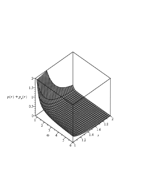
Figure 1: The plot shows that normal matter satisfies the NEC, i.e., $\rho(r)+p_{r}(r)>0$. The specific values $\Phi_{0}=1$, $r_{0}=1$ and $\alpha=3$ are considered. Note that for large values of $r$ and of $\omega$ the NEC tends to zero. See the text for details.

The condition $r-b(r)>0$ is depicted in Fig. 2, also for the specific values of $\Phi_{0}=1$, $r_{0}=1$, $\alpha=3$. The flaring-out restriction, $b^{\prime}(r_{0})<1$ is depicted in Fig. 3 for $r_{0}=1$. Note that for large values of $\omega$ and $\alpha$ we have $b^{\prime}(r_{0})\approx 1$, so that the throat flares out very slowly.

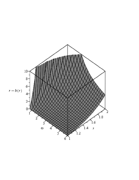
Figure 2: The plot depicts the condition $r-b>0$, with the following values: $r_{0}=1$ and $\alpha=3$.

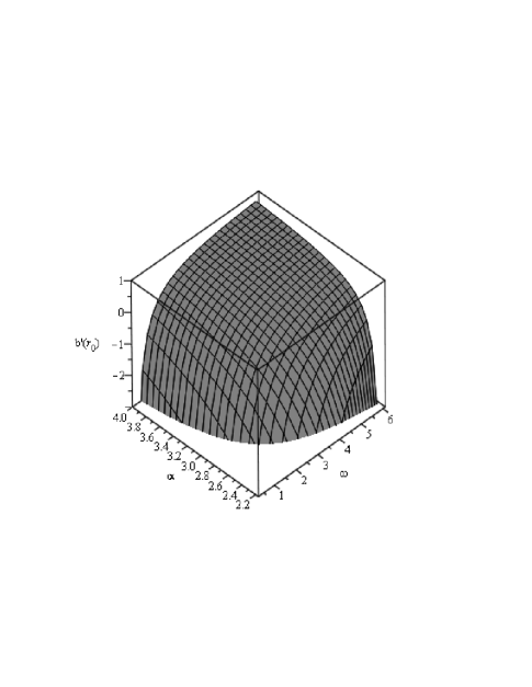
Figure 3: The plot depicts the condition for $b^{\prime}<1$. Note that for large values of $\omega$ and $\alpha$ we have $b^{\prime}(r_{0})\approx 1$, so that the throat flares out very slowly. See the text for details.

IV Conclusion

A fundamental ingredient in wormhole physics is the presence of exotic matter, which involves a stress-energy tensor that violates the null energy condition. A wide range of the solutions have been found in the literature that minimize the usage of exotic matter such as thin shell wormholes, where using the cut-and-paste procedure the exotic matter is minimized and constrained to the throat. In the context of modified theories of gravity, it has also been shown that one can impose that the normal matter satisfies the null energy condition and it is the effective stress-energy tensor, containing higher curvature terms which can be interpreted as a gravitational fluid, that sustain the wormhole geometry.

In this work, we have also found exact wormhole solutions in Brans-Dicke theory where the normal matter threading the wormhole satisfies the null energy condition for a determined parameter range. More specifically, we have imposed a zero redhsift function more computational simplicity and imposed a specific form for the scalar field. We have found that it is the scalar field that plays the part of exotic matter these solutions, which is in clear contrast to the classical general relativistic static wormhole solutions. It would be interesting to analyse time-dependent solutions and work along these lines is in progress.

References

- (1) M. Morris and K. S. Thorne, Am. J. Phys. 56, 395 (1988); M. Morris, K. S. Thorne and U. Yurtsever, Phys. Rev. Lett. 61, 1442 (1988); M. Visser, Lorentzian Wormholes: From Einstein to Hawking (American Institute of Physics, New York, 1995); J. P. S. Lemos, F. S. N. Lobo and S. Quinet de Oliveira, Phys. Rev. D 68, 064004 (2003); F. S. N. Lobo, arXiv:0710.4474 [gr-qc].
- (2) F. J. Tipler, “Energy conditions and spacetime singularities,” Phys. Rev. D 17, 2521 (1978).
- (3) B. Bhawal and S. Kar, Phys. Rev. D 46, 2464-2468 (1992); G. Dotti, J. Oliva, and R. Troncoso, Phys. Rev. D 75, 024002 (2007); H. Maeda and M. Nozawa, Phys. Rev. D 78, 024005 (2008); L. A. Anchordoqui and S. E. P Bergliaffa, Phys. Rev. D 62, 067502 (2000); K. A. Bronnikov and S.-W. Kim, Phys. Rev. D 67, 064027 (2003); M. La Camera, Phys. Lett. B573, 27-32 (2003); F. S. N. Lobo, Phys. Rev. D75, 064027 (2007); R. Garattini and F. S. N. Lobo, Class. Quant. Grav. 24, 2401 (2007); R. Garattini and F. S. N. Lobo, Phys. Lett. B 671, 146 (2009); C. G. Boehmer, T. Harko and F. S. N. Lobo, Phys. Rev. D 76, 084014 (2007); C. G. Boehmer, T. Harko and F. S. N. Lobo, Class. Quant. Grav. 25, 075016 (2008); S. Sushkov, Phys. Rev. D 71, 043520 (2005); F. S. N. Lobo, Phys. Rev. D71, 084011 (2005); F. S. N. Lobo, Phys. Rev. D71, 124022 (2005); J. A. Gonzalez, F. S. Guzman, N. Montelongo-Garcia and T. Zannias, Phys. Rev. D 79, 064027 (2009); A. DeBenedictis, R. Garattini and F. S. N. Lobo, Phys. Rev. D 78, 104003 (2008); F. S. N. Lobo, Phys. Rev. D73, 064028 (2006); N. M. Garcia and T. Zannias, Phys. Rev. D 78, 064003 (2008); F. S. N. Lobo, Phys. Rev. D 75, 024023 (2007); N. Montelongo Garcia and T. Zannias, Class. Quant. Grav. 26, 105011 (2009); F. S. N. Lobo, Class. Quant. Grav. 25, 175006 (2008); T. Harko, Z. Kovacs and F. S. N. Lobo, Phys. Rev. D 78, 084005 (2008); T. Harko, Z. Kovacs and F. S. N. Lobo, Phys. Rev. D 79, 064001 (2009);
- (4) M. Visser, S. Kar and N. Dadhich, Phys. Rev. Lett. 90, 201102 (2003); F. S. N. Lobo and M. Visser, Class. Quant. Grav. 21, 5871 (2004).
- (5) M. Visser, Phys. Rev. D 39 (1989) 3182; M. Visser, Nucl. Phys. B 328 (1989) 203; M. Visser, Phys. Lett. B 242, 24 (1990); S. W. Kim, Phys. Lett. A 166, 13 (1992); S. W. Kim, H. Lee, S. K. Kim and J. Yang, Phys. Lett. A 183, 359 (1993); G. P. Perry and R. B. Mann, Gen. Rel. Grav. 24, 305 (1992); M. S. R. Delgaty and R. B. Mann, Int. J. Mod. Phys. D 4, 231 (1995); E. Poisson and M. Visser, Phys. Rev. D 52 7318 (1995); E. F. Eiroa and G. E. Romero, Gen. Rel. Grav. 36 651-659 (2004); F. S. N. Lobo and P. Crawford, Class. Quant. Grav. 21, 391 (2004); E. F. Eiroa and C. Simeone, Phys. Rev. D 70, 044008 (2004); E. F. Eiroa and C. Simeone, Phys. Rev. D 71, 127501 (2005); M. Thibeault, C. Simeone and E. F. Eiroa, Gen. Rel. Grav. 38, 1593 (2006); F. Rahaman, M. Kalam and S. Chakraborty, Gen. Rel. Grav. 38, 1687 (2006); C. Bejarano, E. F. Eiroa and C. Simeone, Phys. Rev. D 75, 027501 (2007); F. Rahaman, M. Kalam and S. Chakraborti, Int. J. Mod. Phys. D 16, 1669 (2007); E. F. Eiroa and C. Simeone, Phys. Rev. D 76, 024021 (2007); F. Rahaman, M. Kalam, K. A. Rahman and S. Chakraborti, Gen. Rel. Grav. 39, 945 (2007); J. P. S. Lemos and F. S. N. Lobo, Phys. Rev. D 78, 044030 (2008) G. A. S. Dias and J. P. S. Lemos, Phys. Rev. D 82, 084023 (2010); E. F. Eiroa and C. Simeone, Phys. Rev. D 83, 104009 (2011); M. La Camera, Mod. Phys. Lett. A 26, 857 (2011); X. Yue and S. Gao, Phys. Lett. A 375, 2193 (2011);
- (6) F. S. N. Lobo, Phys. Rev. D 75, 064027 (2007); F. S. N. Lobo, Class. Quant. Grav. 25, 175006 (2008); F. S. N. Lobo and M. A. Oliveira, Phys. Rev. D 80, 104012 (2009); N. M. Garcia and F. S. N. Lobo, Phys. Rev. D 82, 104018 (2010); N. M. Garcia and F. S. N. Lobo, Class. Quant. Grav. 28, 085018 (2011).
- (7) L. A. Anchordoqui, S. E. Perez Bergliaffa and D. F. Torres, “Brans-Dicke wormholes in non-vacuum spacetime,” Phys. Rev. D 55, 5226 (1997).
- (8) F. S. N. Lobo and M. A. Oliveira, Phys. Rev. D 81, 067501 (2010).
- (9) A. G. Agnese and M. La Camera, “Wormholes in the Brans-Dicke theory of gravitation,” Phys. Rev. D 51, 2011 (1995).
- (10) K. K. Nandi, B. Bhattacharjee, S. M. K. Alam and J. Evans, “Brans-Dicke wormholes in the Jordan and Einstein frames,” Phys. Rev. D 57, 823 (1998).
- (11) K. K. Nandi, A. Islam and J. Evans, “Brans wormholes,” Phys. Rev. D 55, 2497 (1997);
- (12) A. Bhattacharya, I. Nigmatzyanov, R. Izmailov and K. K. Nandi, “Brans-Dicke Wormhole Revisited,” Class. Quant. Grav. 26 (2009) 235017.
- (13) W. Bruckman and E. Kazes, Phys. Rev. D 16, 261 (1977).
- (14) F. S. N. Lobo, Class. Quant. Grav. 21, 4811 (2004); F. S. N. Lobo, Gen. Rel. Grav. 37, 2023 (2005); F. S. N. Lobo and P. Crawford, Class. Quant. Grav. 22, 4869 (2005); F. S. N. Lobo, Class. Quant. Grav. 23 1525 (2006); J. P. S. Lemos and F. S. N. Lobo, Phys. Rev. D 69, 104007 (2004); F. S. N. Lobo and J. P. Mimoso, Phys. Rev. D 82, 044034 (2010);