Analysis of the coronal green line profiles: evidence of excess blueshifts

Abstract

The coronal green line (Fe XIV 5303 Å) profiles were obtained from Fabry-Perot interferometric observations of the solar corona during the total solar eclipse of 21 June 2001 from Lusaka, Zambia. The instrumental width is about 0.2 Å and the spectral resolution is about 26000. About 300 line profiles were obtained within a radial range of 1.0–1.5 R_⊙ and position angle coverage of about 240°. The line profiles were fitted with single Gaussian and their intensity, Doppler velocity, and line width have been obtained. Also obtained are the centroids of the line profiles which give a measure of line asymmetry. The histograms of Doppler velocity show excess blueshifts while the centroids reveal a pre-dominant blue wing in the line profiles. It has been found that the centroids and the Doppler velocities are highly correlated. This points to the presence of multiple components in the line profiles with an excess of blueshifted components. We have then obtained the(Blue–Red) wing intensity which clearly reveals the second component, majority of which are blueshifted ones. This confirms that the coronal green line profiles often contain multicomponents with excess blueshifts which also depend on the solar activity. The magnitude of the Doppler velocity of the secondary component is in the range 20–40 km s^-1 and they show an increase towards poles. The possible explanations of the multicomponents could be the type II spicules which were recently found to have important to the coronal heating or the nascent solar wind flow, but the cause of the blue asymmetry in the coronal lines above the limb remains unclear.

1 Introduction

The coronal green line Fe XIV 5302.86 Å is the most prominent visible emission line from the inner solar corona and hence it is the most widely observed line during the total solar eclipses. This is because it’s formation temperature is about 1.8 MK which is closer to the average temperature of the inner corona.

Line profile analysis gives information on the physical conditions of the source such as density, temperature, Doppler and nonthermal velocities, wave motions etc. Such analysis on the coronal green line can provide useful insights to the unresolved problems such as the coronal heating and the acceleration of solar wind.

The existence of mass motions in the corona remained controversial in the past. The inner corona was thought to be quiescent with no mass motions greater than a few km s^-1(Newkirk, 1967; Liebenberg et al., 1975; Singh et al., 1982). However, there have been several observations of large-scale motions in the corona (Delone & Makarova, 1969, 1975; Delone et al., 1988; Chandrasekhar et al., 1991; Raju et al., 1993). The later SOHO and TRACE observations have laid to rest this controversy by showing a highly dynamic corona with large velocities and different kinds of wave motions (Brekke, 1999).

It has been known since seventies that the EUV emission lines from the transition region of the quiet Sun are systematically redshifted (Brekke, 1999). The typical value of the average downflow velocity is 5–10 km s^-1. The magnitude of the redshift has been found to increase with temperature and then decrease sharply (Doschek et al., 1976; Hassler et al., 1991; Brekke, 1993). Measurements of this variation is somewhat ambiguous but the recent SUMER results suggest that the upper transition region and lower corona lines are blueshifted, with a steep transition from red to blue shifts above 0.5 MK (Chae et al., 1998; Peter & Judge, 1999). In active regions, multiple flows were observed by Kjeldseth-Moe et al. (1988, 1993). Brekke et al. (1992) obtains multiple Gaussian fits to Si IV 1402 Å profiles with velocities up to 105 km s^-1. Brekke et al. (1997) reports the first observation of large Doppler shifts in individual active region loops above the limb. The high shifts are present only in parts of loops. The line of sight velocities are -60 km s^-1 and 50 km s^-1, so the axial flow velocities could be much higher. A systematic investigation by Kjeldseth-Moe & Brekke (1998) confirmed that high Doppler shifts are common in active region loops. From SUMER observations, Peter (2001) finds that the emission line profiles of the transition region are best-fitted by a double Gaussian with a narrow line core and a broad second component.

The details of line profiles from the corona were difficult to obtain during the SOHO era and before because of instrumental limitations. The spectral resolution of Extreme ultra violet Imaging Spectrometer (EIS; Culhane et al. (2007)) onboard Hindode (Kosugi et al., 2007) is about 4000 which is worse than SUMER but the good signal-to-noise ratio provided the possibility of studying the details of the line profile (see Peter, 2010). Hara et al. (2008) observed asymmetry in the coronal line profiles of Fe XIV 274 Å and Fe XV 284 Å using EIS/HINODE. The excess emission seen in the blue wing has been interpreted in terms of nanoflare heating model by Patsourakos & Klimchuk (2006). De Pontieu et al. (2009) find a strongly blueshifted component in the coronal emission lines which is interpreted as due to type II spicules. Blueshifts of about 30 km s^-1 have been found in coronal lines for plasma in the coronal hole which were interpreted as evidence for nascent solar wind flow (Tu et al., 2005; Tian et al., 2010). Peter (2010) examined line profiles of Fe XV from EIS onboard Hinode and found that the spectra are best fit by a narrow line core and a broad minor component with blueshifts up to 50 km s^-1 . De Pontieu et al. (2011) have used SDO and Hinode observations to reveal ubiquitous coronal mass supply due to acceleration of type II spicules into the corona, which plays a substantial role in coronal heating and energy balance.

As mentioned above, there have been occasional reports of high velocities in the corona even in the pre-SOHO era. These are ground-based eclipse or coronagraphic observations in the visible emission lines made above the limb. The presence of multicomponents with an excess of blueshifts in the coronal green line profiles have been reported (Raju et al., 1993; Raju, 1999). Recently Tyagun (2010) reported similar results in the coronal red line Fe X 6374 Å. In the present paper, we revisit the problem of the velocity field in the corona in the light of new results from SOHO, Hinode etc. We have obtained the coronal green line profiles from Fabry-Perot interferometric observations during the total solar eclipse which have high spectral resolution. In the following sections we describe the data and the analysis steps, results, discussion and conclusions.

2 Data and Analysis

Fabry-Perot interferometric observations of the solar corona were made during the total solar eclipse of 21 June 2001 from Lusaka, Zambia. The instrumental setup is similar to the earlier observations (Chandrasekhar et al., 1984). The free spectral range of the Fabry-Perot interferometer is 4.75 Å and the instrumental width is about 0.2 Å. The spectral resolution at the coronal green line is about 26000.

The analysis involved the following steps; i) locating the fringe center position in the interferogram, ii) radial scans from the fringe center and isolation of fringes, iii) positional identification in the corona, iv) wavelength calibration, v) continuum subtraction, vi) Gaussian fitting to the line profile which gives intensity, linewidth, Doppler velocity.

The centroid of the line profile which is defined as the wavelength point that divides the area of the line profile into two was also obtained. This gives a measure of the line asymmetry if multiple components are present.

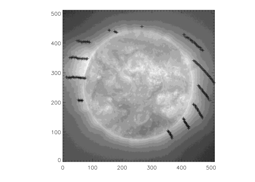
Figure 1: The spatial locations of the line profiles marked on an EIT image of the Sun.

About 300 line profiles within a radial range of 1.0–1.5 R_⊙and position angle coverage of about 240°have been obtained. Only those with a signal-to-noise ratio above 15 were considered in the analysis which limited their number to 272. Those line profiles with a signal-to-noise ratio less than 15 were found to have a larger uncertainty in the background intensity. This in turn affect the accuracy of the Gaussian fitting of the line profiles. The position of the line profiles are marked on an EIT image of the Sun in Figure 1 where the north is up and the west is towards the right. The position angle 0°corresponds to the west while 90°denotes the north pole. The data are scattered because they represent the fringe maxima positions. There is a also gap of about 120°around the south pole.

3 Results and Discussion

In Figure 2, we have shown 30 line profiles alongwith their single Gaussian fits. The estimated errors in the fitting are about 5 % in intensity, 2 km s^-1 in velocity and 0.03 Å in width. The line profiles do not show explicit evidence of multicomponents and the fits are generally seem to be satisfactory.

The radial variations of linewidth, Doppler velocity and centroid of all the line profiles are given in Figure 3. The straight line fits to the radial variations do not show any specific trend. However the variations show a wave-like pattern sometimes. The absence of trend in the width does not agree with some of the earlier results. For example, Singh et al. (2006) find that the width of the green line decreases with coronal height up to about 1.31 Ro and then remain constant. The coronal red line showed an opposite behavior. Chandrasekhar et al. (1991) find a broad peak in the radial variation of the width at about 1.2 R_⊙.

Next we examine the position angle dependence of the radial variations of the Doppler velocity and width. The behavior of two position angle intervals (155–175, -(45–25)) is shown in Figure 4. The other position angle intervals show an intermediate behavior. There is an increase of Doppler velocity and width with respect to the coronal radial distance in the former whereas there is no such dependence in the latter. The wave-like appearance is more prominent in position angle intervals. The result imply that the trend is governed by the underlying activity of the solar region. The increase of the Doppler velocity and width with respect to the coronal radial distance in the first case implies that there is a dependence of Doppler velocity and width which is shown in the lowest panel of Figure 4. The correlation coefficient is rather small(0.29) but significant. The probability that any two random distribution can give a higher correlation coefficient is only 0.03. A positive correlation between Doppler velocity and width could indicate a heating process driving a flow (Peter, 2010).

The histograms of width, Doppler velocity and centroid are shown in Figure 5. The width peaks at 0.9 Å which if it is converted to temperature, is 3.14 MK. Taking the formation temperature of the line to be 1.8 MK, this would imply a nonthermal velocity of 20 km s^-1. The nonthermal velocities in the corona are reported to be in the range of 10–100 km s^-1 which include the possible variations in different coronal regions (Harra-Murnion et al., 1999). The observed average nonthermal velocity of agrees well with reported values. The histograms of Doppler velocity and centroid are similar. Note that both the histograms show a clear excess of blueshifts.

The Doppler velocity versus centroid is given in Figure 6. It can be seen that there is a very strong positive correlation between the two ($q>0.99$). This suggests that there is a secondary component present in the line profile because if it is not the case, then the relationship between the velocity and the centroid will be random. Also the straight-line relationship seen in both the negative and positive quadrants means that there are both blueshifts and redshifts present in the line profile. Hence the results, in general, point to the multicomponent-nature of the coronal green line profiles.

In order to see the nature of the secondary component, we have obtained the (Blue–Red) wing intensity of the line profiles which is plotted in Figure 7. Only the blue-wing is shown in the Figure. This will bring out the secondary component in the line profiles - the positive component represents the blueshift whereas the negative one gives the redshift. The statistics is given in Table 1. Clearly there is an excess of blueshifts over redshifts. Also, for most of the line profiles in column 1, it is difficult to decide whether they are single or multiple because the secondary component is weak which are then put together as single/ambiguous. A Gaussian fit to the secondary component is also shown in the Figure which gives the relative intensity, Doppler velocity and the width. Details of the fitting procedure are given in Table 2. The relative intensity of the secondary component could be up to 54 %, Doppler velocity $\pm$ (20–40) km s^-1, and width 0.5–0.8 Å.

It can be seen that there is a consistent picture emerges from Figures 5–7 and Tables 1–2. The histograms of width and centroid in Figure 5 show that there is an excess of blueshifts and a prominent blue asymmetry in the line profiles. The high positive correlation between the Doppler velocity and centroid in Figure 6 implies the presence of multiple components within the line profiles. Figure 7 confirms that the multicomponents are real and not any artifacts of the fitting procedure. Also Table 1 confirms that the prominent blue asymmetry arises because of the excess blueshifts in the line profiles. This can be further seen in Table 2. When the single Gaussian fit gives indication of (negative/positive) Doppler velocity, there is a (blue/red) secondary component present in the line profile. This would imply that the parameters obtained through the single Gaussian fitting of the line profiles are only indications of the actual values. The Doppler velocities obtained could be underestimates of the relative line-of-sight velocities between the main and secondary components. Similarly the obtained widths may be overestimates of the individual widths of the components.

The evidence of blue asymmetry in the coronal line profiles was first pointed out by (Raju et al., 1993). The multicomponents were explained on the basis of mass motions in the coronal loops(Raju, 1999), though the blue asymmetry remained as a puzzle. The occurrence of multicomponents in the coronal line profiles was found to depend upon the solar activity. The line profiles of 1980 solar maximum corona (monthly sunspot number = 155) showed strong multicomponents, sometimes up to 4. The relative velocities between multicomponents were found to go up to 70 km s^-1. On the other hand the line profiles of 1983 corona which belong to a declining solar activity phase (monthly sunspot number = 91), showed mostly single Gaussians but sometimes double Gaussians and rarely triple Gaussians (Chandrasekhar et al., 1991). The year 2001 belongs to the solar maximum phase but the activity was lower (monthly sunspot number = 134) as compared to 1980. Here the line profiles are mostly double Gaussians and relative velocities are about 30 km s^-1. Similar results are also observed for coronal red line, Fe X 6374 Å. From a single Gaussian analysis of Norikura coronagraph data, Raju et al. (2000) find that though the majority of Doppler velocities are only a few km s^-1, there is a definite excess of blueshifts over redshifts. Also, Tyagun (2010) from an analysis of about 5500 line profiles belong to 1968-72 reported that 80 % of the coronal red line profiles are asymmetric and the fractions of the asymmetric profiles with more intense blue and red wings are 52 and 28 % respectively. To summarize, the line profiles of coronal visible emission lines often show multicomponents with a predominant blue wing. The occurrence of multicomponents show a dependence on solar activity.

Now what are the possible causes of the blue asymmetry. The differential rotation of the Sun can cause preferential blueshifts at the east limb and redshifts at the west limb. But the maximum velocity is only 2 km s^-1which is comparable to the error involved and hence may not be detected. The recent results from SOHO and HINODE show evidence of multiple components and a predominant blue wing in the EUV emission linesHara et al. (2008); De Pontieu et al. (2009); Peter (2010). De Pontieu et al. (2011) have explained this on the basis of upflows due to type II spicules which have implications to coronal heating. It is possible that the secondary component with a preferential blueshift could be due to the type II spicules. The blueshifts are also explained as due to the nascent solar wind flow (Tu et al., 2005; Tian et al., 2010). It should be noted that the above observations are mostly made on the disk. The interpretation of the off-limb results is even more complicated due to the line-of-sight effects. The upflows can cause blueshift, redshift or no shift in a line profile depending on the angle between the flow and the plane of the sky. It may be noted that Hara et al. (2008) find excess blueshifts at the disk center which gradually disappear near the limb. Tian et al. (2010) explain the redshifts of Fe XII and Fe XIII lines at the limb on the basis of tilt of the solar rotation axis (B0). Our observations are made on June 21 when B0 = 1.8. If the flows are assumed to be radial, this may cause a slight preferential blueshift at the north pole and redshift at the south pole. However we have not seen any preferential blue/redshifts seen at the poles. We have examined the dependence of Doppler velocity of the secondary component on the position angle which is shown in Figure 8. It may be seen that the velocities show a dependence on the position angle with a maxima at the poles and minima at the equator. This is akin to the behavior of the solar wind flow. It is well-known that the fast wind emanates from the coronal holes of polar regions whereas the slow wind comes from the streamer structures in the equatorial regions. Also it is suggested that an asymmetric velocity distribution of the emitting ions could cause line asymmetries (Peter, 2010). It may be seen that the results fit well with the overall behavior of the solar atmosphere; that the redshifts in the lower transition region slowly changes sign to blueshifts in the upper transition region which continues to increase in the lower corona.

The above discussion points to the fact that the velocity field in the corona is quite complex. There are evidences of wave motions, mass motions in coronal loops, solar wind flow, and type II spicular flows. Their detailed nature and significance are yet to be understood. We may expect that HINODE observations of line profiles from both the disk and the limb will give more insights on this.

4 Conclusions

It has been shown that the coronal green line profiles, in general, contains multicomponents. Though the single Gaussian fitting gives a definite indication of the of multicomponents, the parameters obtained such as the Doppler velocity and the width could be under/over-estimates of the actual values. The occurrence of multicomponents has been found to be related the solar activity. It has also been found that there is a definite blue asymmetry meaning an excess of blueshifts over redshifts in the coronal line profiles. The causes of the blue asymmetry are not clear but future HINODE observations of both disk and limb may resolve this.

Figure 2: Intensity (arbitrary units) plotted against wavelength difference from peak (Å) for 30 line profiles. Single Gaussian fittings are given as the continuous line. The fitted parameters are given in Table 2.

Figure 3: Radial variations of linewidth, Doppler velocity and centroid. The solid line represents the straight line fit.

Figure 4: Doppler velocity and width are plotted against coronal radial distance for two position angles in the two upper panels. Doppler velocity vs width is plotted in the lowest panel. The solid line represents the straight line fit. The numbers indicate the position angle interval, number of points, correlation coefficient and the probability that any two random distribution can give a higher correlation coefficient.

Figure 5: Histograms of width, Doppler velocity and centroid.

Figure 6: Doppler velocity plotted against centroid. The solid line represents the straight line fit.

Figure 7: The (Blue–Red) wing intensity of the same line profiles as of Figure 2. The solid line represents the Gaussian fit. The fitted parameters are given in Table 2. The upper 10 profiles represent single/Ambiguous, the middle 10 represent blueshifted components and the lower 10 represent redshifted components.

Figure 8: Doppler velocity of the secondary component plotted against position angle. The solid line represents a polynomial fit.

Table 1: Number of single/multicomponents. The numbers given in the bracket give the percentage.

Single/Ambiguous	Blue	Red	Total
114	93	65	272
(42)	(34)	(24)	(100)

Table 2: Details of Gaussian fitting. Columns 2–4 give the parameters of single Gaussian fitting. Columns 5–7 give the parameters of Gaussian fitting of the blue component shown in 3–4 rows of Figure 6. Columns 8–10 give the parameters of Gaussian fitting of the red component shown in last 2 rows of Figure 7.

	Single Gaussian			Blue			Red
No.	Int	Vel	Wid	Int	Vel	Wid	Int	Vel	Wid
1	1.00	-0.65	0.95
2	1.00	-1.62	0.94
3	1.00	0.88	0.88
4	1.00	0.72	0.90
5	1.00	-0.49	0.92
6	1.00	-0.06	0.84
7	1.00	-0.40	0.87
8	1.00	-0.37	0.91
9	1.00	-0.67	0.89
10	1.00	-0.24	0.95
11	1.00	-7.00	0.89	0.36	-23.75	0.65
12	1.00	-4.57	0.86	0.27	-24.95	0.53
13	1.00	-5.11	0.96	0.28	-26.13	0.55
14	1.00	-4.08	0.97	0.24	-25.37	0.48
15	1.00	-5.26	0.89	0.29	-28.98	0.58
16	1.00	-8.71	0.96	0.47	-25.85	0.55
17	1.00	-9.17	0.92	0.52	-27.35	0.58
18	1.00	-4.32	0.84	0.27	-21.26	0.50
19	1.00	-7.81	0.91	0.41	-24.86	0.57
20	1.00	-10.46	0.92	0.61	-26.90	0.46
21	1.00	9.08	1.03				-0.39	-26.39	0.79
22	1.00	4.74	0.93				-0.23	-32.37	0.74
23	1.00	6.94	0.98				-0.40	-30.68	0.52
24	1.00	10.59	0.93				-0.54	-31.47	0.65
25	1.00	4.92	0.89				-0.24	-25.00	0.65
26	1.00	9.97	0.91				-0.51	-27.50	0.63
27	1.00	5.85	0.87				-0.31	-23.44	0.64
28	1.00	11.26	1.00				-0.57	-29.84	0.63
29	1.00	9.39	0.98				-0.46	-28.14	0.67
30	1.00	10.47	1.01				-0.54	-26.45	0.56

References

- Brekke (1993) Brekke, P. 1993, ApJ, 408, 735
- Brekke (1999) Brekke, P. 1999, Sol. Phys., 190, 379
- Brekke et al. (1997) Brekke, P., Kjeldseth-Moe, O., & Harrison, R. A. 1997, Sol. Phys., 175, 511
- Brekke et al. (1992) Brekke, P., Brynildsen, N., Kjeldseth-Moe, O., Maltby, P., & Brueckner, G. E. 1992, Study of the Solar-Terrestrial System, 346, 211
- Chae et al. (1998) Chae, J., Yun, H. S., & Poland, A. I. 1998, ApJS, 114, 151
- Chandrasekhar et al. (1991) Chandrasekhar, T., Desai, J. N., Ashok, N. M., & Pasachoff, J. M. 1991, Sol. Phys., 131, 25
- Chandrasekhar et al. (1984) Chandrasekhar, T., Ashok, N. M., Desai, J. N., Pasachoff, J. M., & Sivaraman, K. R. 1984, Appl. Opt., 23, 508
- Culhane et al. (2007) Culhane, J. L., et al. 2007, Sol. Phys., 243, 19
- De Pontieu et al. (2009) De Pontieu, B., McIntosh, S. W., Hansteen, V. H., & Schrijver, C. J. 2009, ApJ, 701, L1
- De Pontieu et al. (2011) De Pontieu, B., et al. 2011, Science, 331, 55
- Delone & Makarova (1969) Delone, A. B., & Makarova, E. A. 1969, Sol. Phys., 9, 116
- Delone & Makarova (1975) Delone, A. B., & Makarova, E. A. 1975, Sol. Phys., 45, 157
- Delone et al. (1988) Delone, A. B., Makarova, E. A., & Iakunina, G. V. 1988, Journal of Astrophysics and Astronomy, 9, 41
- Doschek et al. (1976) Doschek, G. A., Bohlin, J. D., & Feldman, U. 1976, ApJ, 205, L177
- Hara et al. (2008) Hara, H., Watanabe, T., Harra, L. K., Culhane, J. L., Young, P. R., Mariska, J. T., & Doschek, G. A. 2008, ApJ, 678, L67
- Harra-Murnion et al. (1999) Harra-Murnion, L. K., Matthews, S. A., Hara, H., & Ichimoto, K. 1999, A&A, 345, 1011
- Hassler et al. (1991) Hassler, D. M., Rottman, G. J., & Orrall, F. Q. 1991, ApJ, 372, 710
- Kjeldseth-Moe & Brekke (1998) Kjeldseth-Moe, O., & Brekke, P. 1998, Sol. Phys., 182, 73
- Kjeldseth-Moe et al. (1988) Kjeldseth-Moe, O., et al. 1988, ApJ, 334, 1066
- Kjeldseth-Moe et al. (1993) Kjeldseth-Moe, O., Brynildsen, N., Brekke, P., Maltby, P., & Brueckner, G. E. 1993, Sol. Phys., 145, 257
- Kosugi et al. (2007) Kosugi, T., et al. 2007, Sol. Phys., 243, 3
- Liebenberg et al. (1975) Liebenberg, D. H., Bessey, R. J., & Watson, B. 1975, Sol. Phys., 44, 345
- Newkirk (1967) Newkirk, G., Jr. 1967, ARA&A, 5, 213
- Patsourakos & Klimchuk (2006) Patsourakos, S., & Klimchuk, J. A. 2006, ApJ, 647, 1452
- Peter (2001) Peter, H. 2001, A&A, 374, 1108
- Peter (2010) Peter, H. 2010, A&A, 521, A51
- Peter & Judge (1999) Peter, H., & Judge, P. G. 1999, ApJ, 522, 1148
- Raju (1999) Raju, K. P. 1999, Sol. Phys., 185, 311
- Raju et al. (1993) Raju, K. P., Desai, J. N., Chandrasekhar, T., & Ashok, N. M. 1993, MNRAS, 263, 789
- Raju et al. (2000) Raju, K. P., Sakurai, T., Ichimoto, K., & Singh, J. 2000, ApJ, 543, 1044
- Singh et al. (1982) Singh, J., Saxena, A. K., & Bappu, M. K. V. 1982, Journal of Astrophysics and Astronomy, 3, 249
- Singh et al. (2006) Singh, J., Sakurai, T., & Ichimoto, K. 2006, ApJ, 639, 475
- Tian et al. (2010) Tian, H., Tu, C., Marsch, E., He, J., & Kamio, S. 2010, ApJ, 709, L88
- Tu et al. (2005) Tu, C.-Y., Zhou, C., Marsch, E., Xia, L.-D., Zhao, L., Wang, J.-X., & Wilhelm, K. 2005, Science, 308, 519
- Tyagun (2010) Tyagun, N. F. 2010, Geomagnetism and Aeronomy/Geomagnetizm i Aeronomiia, 50, 860