Spin-phonon coupling in single Mn doped CdTe quantum dot

Abstract

The spin dynamics of a single Mn atom in a laser driven CdTe quantum dot is addressed theoretically. Recent experimental resultsLe-Gall_PRL_2009 ; Goryca_PRL_2009 ; Le-Gall_PRB_2010 show that it is possible to induce Mn spin polarization by means of circularly polarized optical pumping. Pumping is made possible by the faster Mn spin relaxation in the presence of the exciton. Here we discuss different Mn spin relaxation mechanisms. First, Mn-phonon coupling, which is enhanced in the presence of the exciton. Second, phonon-induced hole spin relaxation combined with carrier-Mn spin flip coupling and photon emission results in Mn spin relaxation. We model the Mn spin dynamics under the influence of a pumping laser that injects excitons into the dot, taking into account exciton-Mn exchange and phonon induced spin relaxation of both Mn and holes. Our simulations account for the optically induced Mn spin pumping.

I Introduction

The tremendous progress in the miniaturization of electronic devices has reached the point that makes it crucial to address the effect of a single dopant in a device and motivates the study of a single dopant spin to store digital informationSolotronics . The manipulation of a single atom spin in a solid state environment has been demonstrated using several approaches, like scanning tunneling microscope on magnetic adatoms Hirjibehedin_2007 ; Loth_2010 , or optical probing of NV centers in diamond Jelezko2004 and single magnetic atoms in semiconductor quantum dots, the topic of this paper. Single quantum dots doped with a single Mn atom can be probed by means of single exciton spectroscopy in photoluminescence (PL) experiments. This has been done both in II-VI Besombes_PRL_2004 ; Besombes2005 ; Leger05 ; Leger05B ; Leger_PRL_2006 ; Leger_PRB_2007 ; Besombes_PRB_2008 ; Le-Gall_PRL_2009 ; Goryca_PRL_2009 ; Le-Gall_PRB_2010 ; Goryca_PRB_2010 and III-V Kudelski_PRL_2007 ; Krebs_PRB_2009 materials. In the case of single Mn doped CdTe dots, information about the quantum spin state of a single Mn atom is extracted from the single exciton quantum dot photoluminescence due to the one on one relation between photon energy and polarization and the electronic spin state of the Mn atom Fernandez-Rossier_PRB_2006 ; Qu05 ; Govorov04 ; Bhatta ; Bhatta2007 ; Kuhn09 ; Kuhn11 ; JFR04 ; Joost08 . This has made it possible to measure the spin relaxation time of a single Mn atom in a quantum dot under optical excitation, using photon autocorrelation measurementsBesombes_PRB_2008 , and to realize the optical initialization and readout of the spin of the Mn atomLe-Gall_PRL_2009 ; Goryca_PRL_2009 ; Le-Gall_PRB_2010 .

The observation of Mn spin orientation under quasi-resonant optical pumping Le-Gall_PRL_2009 ; Goryca_PRL_2009 ; Le-Gall_PRB_2010 can be accounted for if the Mn spin relaxation time is shorter in the presence of a quantum dot exciton Govorov05 ; Le-Gall_PRB_2010 ; Cao10 ; Cywinski10 . In that situation, resonant excitation of an optical transition associated to a given Mn spin projection results in the depletion of the laser driven Mn spin state, via Mn spin relaxation in the presence of the exciton. Whereas theoretical understanding of the exchange couplings between electrons, holes and Mn spin in quantum dots permits to account for the observed PL spectra Besombes_PRL_2004 ; Leger05 ; Leger05B ; Fernandez-Rossier_PRB_2006 , a complete understanding of the spin dynamics under the combined action of laser pumping, incoherent spin relaxation and coherent spin-flips is still missing. In this paper we make progress along this direction on two counts. First, we discuss different Mn spin relaxation mechanism, taking fully into account the interplay between incoherent dynamics due to the coupling to a reservoir and the coherent spin flips associated to exciton-Mn exchange in the quantum dot. Our calculations show that the most efficient Mn spin relaxation channel, in the presence of the exciton, arises from a combination of phonon-induced hole spin relaxation, which turns the bright exciton into a dark, followed by recombination to the ground enabled by dark-bright mixing due to Mn-carrier spin flip exchange. Thus, we provide a quantitative basis to a recently proposed scenarioCywinski10 . Second, we model the Mn spin dynamics with a rate equation for the Mn spin and the Mn plus exciton spin states that includes the spin relaxation rates between the few-body states calculated from microscopic theory.

Our theory permits to model the experimental observations and, importantly, it identifies the light-hole heavy-hole mixing as a crucial parameter that determines not only the PL lineshape Leger05 ; Leger05B ; Fernandez-Rossier_PRB_2006 but also the amplitude of several spin-relaxation mechanisms at play in this system.

The rest of this manuscript is organized as follows. In section II we review the Hamiltonian for a single Mn spin interacting with a single exciton in a quantum dot. The anisotropic Mn-hole coupling is derived from a simplifieddot-holes ; Fernandez-Rossier_PRB_2006 single-particle description of the lowest energy quantum dot hole states which affords analytical expressions for the critical parameter in the theory, the light-hole heavy hole (LH-HH) mixing dot-holes . The dependence of the properties of the Mn-exciton states on the LH-HH mixing are discussed. In section (III) we discuss the Mn spin relaxation due to Mn-phonon coupling, both with and without an exciton in the quantum dot. Whereas this mechanism is probably dominant for the Mn spin relaxation in the optical ground state, it is not sufficient to account for the rapid Mn spin relaxation in the presence of the exciton. This leads us to consider other spin relaxation mechanisms. In section (IV) we describe the spin relaxation of holes due to their coupling to acoustic phonons, using a Bir-Pikus Hamiltonian. Using the simplified description of hole states, we obtain analytical results for the hole spin lifetime in a non-magnetic dot, which are in agreement with previous work using a more sophisticated description of single hole states Woods04 . We then compute the lifetime of the exciton-Mn states due to hole spin relaxation. In section (VI) we present our simulations of the optical pumping process, using rate equations for the exciton-Mn quantum states, including the laser pumping, the spontaneous photon emission, the Mn and hole spin relaxation due to phonons. Our simulations account for the optical initialization and readout observed experimentally.

II Exciton-$\rm Mn$ Hamiltonian

In this section we describe a minimal Hamiltonian model that can accounts for the PL spectra of single Mn doped CdTe quantum dots. For that matter we need to consider both the Mn spin in the unexcited crystal and the Mn spin interacting with a quantum dot exciton. The peaks in the PL spectra are associated to the energy differences between the states of the dot with and without the exciton.

II.1 Mn spin Hamiltonian

Mn is a substitutional impurity in the Cd site of CdTe. Thus, it has an oxidation state of $2+$, so that the 5 $d$ electrons have spin $S=\frac{5}{2}$, resulting in a sextupletFurdyna whose degeneracy is lifted by the interplay of spin orbit and the crystal field. In an unstrained CdTe, the crystal field has cubic symmetry which should result in a magnetic anisotropy Hamiltonian without quadratic terms. Electron paramagnetic resonance (EPR) in CdTe strained epilayersQazzaz show that Mn has an uniaxial term in the spin Hamiltonian. In a quantum dot there could be some in-plane anisotropy as well, which lead us to consider the following Hamiltonian:

$${\cal H}_{0}=DM_{z}^{2}+E(M_{x}^{2}-M_{y}^{2})+g\mu_{B}\vec{B}\cdot\vec{M}$$ (1)

where $M_{a}$ are the $S=\frac{5}{2}$ spin operators of the electronic spin of the Mn. The eigenstates of this Hamiltonian are denoted by $\phi_{m}$

$${\cal H}_{0}|\phi_{m}\rangle=E_{m}|\phi_{m}\rangle=E_{m}\sum_{M_{z}}\phi_{m}(M_{z})|M_{z}\rangle$$ (2)

where $|M_{z}\rangle$ are the eigenstates of $M_{z}$. In this paper we neglect the hyperfine coupling to the $I=\frac{5}{2}$ nuclear spin, which could affect the decay of the electronic spin coherence Le-Gall_PRL_2009 . The magnetic anisotropy parameters, $E$ and $D$ can not be inferred from PL experiments, which are only sensitive to the Mn-exciton coupling. EPR experimentsQazzaz in strained layer could be fit with $D=12\mu$eV, $E=0$ and $g=2.0$. Thus, the ground state should have $M_{z}=\pm\frac{1}{2}$, split from the first excited state by $2D$. At 4 Kelvin and zero magnetic field, we expect all the six spin levels to be almost equally populated. We refer to these six states as the ground state manifold , in contrast to the excited state manifold, which we describe with 24 states corresponding to 4 possible quantum dot exciton states and the 6 Mn spin states.

II.2 Single particle states of the quantum dot

We describe the confined states of the quantum dot with a simple effective mass model. In the case of the conduction band electrons, we neglect spin orbit coupling and we only consider the lowest energy orbital, with wave function $\psi_{0}(\vec{r})$, which can accommodate 1 electron with two spin orientations.

In the case of holes, spin orbit coupling lifts the sixfold degeneracy of the top of the valence band into a $J=\frac{3}{2}$ quartet and a $J=\frac{1}{2}$ doublet which, in CdTe, is more than 0.8eV below in energy. Confinement and strain lift the fourfold degeneracy of the $J=\frac{3}{2}$ hole states, giving rise to a mostly $J_{z}=\pm\frac{3}{2}$ heavy hole doublet and a almost $J_{z}=\pm\frac{1}{2}$ light hole doublet. Importantly, it is crucial to include LH-HH mixing to describe the experimental observation.

II.2.1 Effect of confinement

The top of the valence band states are described in the kp approximation with the so called Kohn-Luttinger Hamiltonian Kohn-Luttinger ; Broido-Sham . For that matter, the crystal Hamiltonian is represented in the basis of the 4 topmost $J=\frac{3}{2}$ valence states of the $\Gamma$ point. We label them by $J=\frac{3}{2},J_{z}$. The resulting kp Hamiltonian can be written as ${\cal H}_{\rm holes}={\cal H}_{\rm KL}$

$${\cal H}_{\rm KL}=\sum_{i,j=x,y,z}V^{\rm KL}_{ij}J_{i}J_{j}k_{i}k_{j}+\kappa\mu_{B}J_{z}B$$ (3)

where $k_{i}$ are the wave vectors, $J_{i}$ are the spin $\frac{3}{2}$ matrices, and $V^{\rm KL}_{ij}$ are coefficients given in the appendix 88. The last term accounts for the Zeeman coupling to an external field along the growth direction.

The kp Hamiltonian for states in the presence of a quantum dot confinement potential that breaks translational invariance reads:

$${\cal H}_{\rm kp}=-\hbar^{2}\sum_{i,j=x,y,z}V^{\rm KL}_{ij}J_{i}J_{j}\partial_{i}\partial_{j}+\kappa\mu_{B}J_{z}B+V(\vec{r})\delta_{j_{z},j_{z}^{\prime}}$$ (4)

In general, the numerical solution of equation (4) can be very complicated. Following previous workdot-holes ; Fernandez-Rossier_PRB_2006 , we make two approximations that permit to obtain analytical solutions. First, we model the quantum dot with a hard-wall box-shape potential. The dimensions of the box are $L_{x}$, $L_{y}$ and $L_{z}$. This permits to write the wave function as a linear combination of $|J=\frac{3}{2},J_{z}\rangle$ states multiplied by the confined waves

$$\psi_{\vec{n}}(\vec{r})=\sqrt{\frac{8}{V}}Sin\left(\frac{n_{x}\pi x}{L_{x}}\right)Sin\left(\frac{n_{y}\pi y}{L_{y}}\right)Sin\left(\frac{n_{z}\pi z}{L_{z}}\right)$$ (5)

Our second approximation is to restrict the basis set to the fundamental mode only, $n_{x}=n_{y}=n_{z}=1$. As a result, the quantum dot Hamiltonian reads

$${\cal H}_{\rm kp}=-\hbar^{2}\sum_{i,j=x,y,z}V^{\rm KL}_{ij}J_{i}J_{j}\langle\partial_{i}\partial_{j}\rangle$$ (6)

where

$$\langle\partial_{i}\partial_{j}\rangle=\int\psi_{1,1,1}(\vec{r})\partial_{i}\partial_{j}\psi_{1,1,1}(\vec{r})=\delta_{ij}\left(\frac{2\pi}{L_{i}}\right)^{2}$$ (7)

Thus, within this approximation, the quantum dot hole states are described by a 4*4 Kohn Luttinger Hamiltonian where the terms linear in $k_{i}$ vanish and the $k_{i}^{2}$ terms are replaced by $\left(\frac{2\pi}{L_{i}}\right)^{2}$. The resulting matrix ${\cal H}_{\rm conf}$ has two decoupled sectors denoted by $+$ ($J_{z}=+\frac{3}{2}$,$J_{z}=-\frac{1}{2}$) and $-$ ($J_{z}=-\frac{3}{2}$,$J_{z}=+\frac{1}{2}$). In the $(+\frac{3}{2},-\frac{1}{2},+\frac{1}{2},-\frac{3}{2})$ basis we have:

$${\cal H}_{\rm conf}=\left(\begin{array}[]{cc}{\cal H}_{+}&0\\ 0&{\cal H}_{-}\end{array}\right)$$ (8)

with

$${\cal H}_{+}=\left(\begin{array}[]{cc}\overline{P}+\overline{Q}-\frac{3b}{2}&\overline{R}\\ \overline{R}&\overline{P}-\overline{Q}+\frac{b}{2}\end{array}\right)$$ (11)

and

$${\cal H}_{-}=\left(\begin{array}[]{cc}\overline{P}-\overline{Q}-\frac{b}{2}&\overline{R}\\ \overline{R}&\overline{P}+\overline{Q}+\frac{3b}{2}\end{array}\right)$$ (14)

where $b\equiv\kappa\nu_{B}B$ and $\overline{P}$, $\overline{Q}$ and $\overline{R}$ are given in the appendix. In order to find the corresponding energies and wavefunctions it is convenient to write these matrices as: ${\cal H}_{\pm}=a_{\pm}+\vec{h}_{\pm}\cdot\vec{\sigma}$ where $\vec{\sigma}$ are the Pauli matrices acting on the pseudospin $\frac{1}{2}$ space of the $+$ and $-$ spaces, $a_{\pm}=P\mp b/2$ and

$$\vec{h}_{\pm}=\left(\overline{R},0,\overline{Q}\mp b\right)=|\vec{h}_{\pm}|\left(Sin\theta_{\pm},0,Cos\theta_{\pm}\right)$$ (15)

We keep only the two ground states (heavy-hole like), denoted by $|\Uparrow\rangle$ and $|\Downarrow\rangle$, which are several meV away from the light-hole like states. The ground state doublet for the quantum dot holes states so obtained, neglecting strain, can be written as

$$|\Uparrow\rangle = cos\frac{\theta_{+}}{2}|+\frac{3}{2}\rangle+sin\frac{\theta_{+}}{2}|-\frac{1}{2}\rangle$$

$$|\Downarrow\rangle = cos\frac{\theta_{-}}{2}|+\frac{-3}{2}\rangle+sin\frac{\theta_{-}}{2}|+\frac{1}{2}\rangle$$ (16)

Thus, the LH-HH mixing parameters, $\theta_{\pm}$ depend on the dot dimension, $L_{i}$, on the Kohn Luttinger parameters, $\gamma_{i}$ and on the applied magnetic field $B$.

II.2.2 Effect of homogeneous strain

We now consider the effect of the strain that arises from the lattice mismatch between the CdTe quantum dot and the ZnTe substrate on the $J=\frac{3}{2}$ states of the valence band. It has a similar effect that confinement, resulting in a splitting of the $J=\frac{3}{2}$ manifold and a mixing of the LH and HH states. The Hamiltonian that describes the effect of strain, as described by the strain tensor $\epsilon_{ij}$, on the top of the valence band states in zinc-blende semiconductors was proposed by Bir and Pikus. We can write the Bir and Pikus (BP) Hamiltonian as Cardona-Yu :

$${\cal H}_{\rm BP}=\left(a-\frac{9b}{4}\right)(e_{xx}+e_{yy}+e_{zz})+$$

$$+3b\sum_{i=x,y,z}J_{i}^{2}e_{ii}+\sqrt{3}d\left(\left(J_{x}J_{y}+J_{y}J_{x}\right)e_{xy}+{\rm c.p.}\right)$$ (17)

where ${\rm c.p.}$ stands for cyclic permutation, and $a=-3.4$eV, $b=-1.2$eV, $d=-5.4$eV for CdTeCardona-Yu .

For CdTe quantum dots grown in ZnTe, we mainly consider the effects of strain anisotropy in the growth planeLeger_PRB_2007 and describe the strain by the average values of $e_{xy}$ and $e_{xx}-e_{yy}$. In this approximation the BP Hamiltonian is reduced to a block diagonal matrix in the $(+\frac{3}{2},-\frac{1}{2},+\frac{1}{2},-\frac{3}{2})$ basis:

$${\cal H}_{BP}=\left(\begin{array}[]{cc}{\cal H}_{BP+}&0\\ 0&{\cal H}_{BP-}\end{array}\right)$$ (18)

where

$${\cal H}_{BP+}=\left(\begin{array}[]{cc}0&\rho_{s}e^{-2i\varphi_{s}}\\ \rho_{s}e^{2i\varphi_{s}}&\Delta_{lh}\end{array}\right)$$ (19)

$${\cal H}_{BP-}=\left(\begin{array}[]{cc}\Delta_{lh}&\rho_{s}e^{-2i\varphi_{s}}\\ \rho_{s}e^{2i\varphi_{s}}&0\end{array}\right)$$ (20)

where $\Delta_{lh}$ is the HH-LH splitting, $\rho_{s}$ the strained induced amplitude of the HH-LH mixing and $\phi_{s}$ the angle between the strained induced anisotropy axis in the quantum dot plane and x (100) axis. Importantly, the effect of confinement and the effect of strain have a very similar mathematical structure. They both split the LH and HH levels and mix them. The main difference lies in the mixing term, which is real for the confinement Hamiltonian controlled by the shape of the quantum dot and complex for the BP Hamiltonian depending on the strain distribution in the quantum dot plane.

II.2.3 Combined effect of confinement and strain

We finally consider the combined action of confinement and strain described by ${\cal H}_{\rm holes}={\cal H}_{\rm conf}+{\cal H}_{BP}$. Summing the Hamiltonians of equations (8) and (18) to obtain two decoupled matrices for the $+$ and $-$ subspaces. They can be written as

$${\cal H}_{\rm tot,\pm}=A_{\pm}+\vec{H}_{\pm}\cdot\vec{\sigma}$$ (21)

where $A_{\pm}=\overline{P}\mp\frac{b}{2}+\frac{\Delta_{lh}}{2}$ and

$$\vec{H}_{\pm}=$$

$$\left(\overline{R}+\rho_{s}cos(2\varphi_{s}),\pm\rho_{s}sin(2\varphi_{s}),\overline{Q}\mp b-\frac{\Delta_{lh}}{2}\right)$$ (22)

It is convenient to express the ground state doublet associated to ${\cal H}_{\rm holes}$ in terms of the spherical coordinates of the vectors $\vec{H}_{\pm}$, $|\vec{H}_{\pm}|$, $\theta_{\pm}$ and $\phi_{\pm}$:

$$|\Uparrow\rangle = Cos\frac{\theta_{+}}{2}|\frac{+3}{2}\rangle-Sin\frac{\theta_{+}}{2}e^{i\phi_{+}}|\frac{-1}{2}\rangle$$

$$|\Downarrow\rangle = Cos\frac{\theta_{-}}{2}|\frac{-3}{2}\rangle-Sin\frac{\theta_{-}}{2}e^{i\phi_{-}}|\frac{+1}{2}\rangle$$ (23)

where

$$e^{i\phi_{\pm}}=\frac{\overline{R}+\rho_{s}e^{\pm 2i\varphi_{s}}}{|\overline{R}+\rho_{s}e^{\pm 2i\varphi_{s}}|}$$ (24)

Expectedly, this expression is formally very similar to that of equation (16).

Formally, we express eq. (23) as

$$|\sigma_{h}\rangle=\sum_{j_{z}}C_{h}(j_{z})|j_{z}\rangle$$ (25)

Both in equations (16) and (23) the ($+\frac{3}{2},-\frac{1}{2}$) sector is decoupled from the ($-\frac{3}{2},+\frac{1}{2}$). Whereas, this is not true in general, it is sufficient to account for the correct symmetry of a variety of exchange couplings between the hole and both the Mn and the electrons.

II.3 Effective Mn-carrier exchange Hamiltonian

II.3.1 Hole-Mn Hamiltonian

We now consider the exchange coupling of hole spin ($\vec{J}$) and the Mn spin ($\vec{M}$). The leading term in the exchange interaction is the Heisenberg operatorFurdyna ; Benoit :

$${\cal V}_{\rm exch}=\beta\delta(\vec{r}_{h}-\vec{r}_{M})\vec{J}\cdot\vec{M}$$ (26)

where $\beta$ is the hole-Mn exchange coupling constant. For Mn in CdTe we have $\beta N_{0}=$0.88 eV, where $N_{0}$ is the volume of the CdTe unit cellFurdyna . The exchange interaction is taken as short ranged, the Mn atom is located at $\vec{r}_{Mn}$ and $\vec{J}$ are the spin $\frac{3}{2}$ angular momentum matrices. We represent the operator (26) in the product basis $|M\rangle\times\sigma_{h}$. Thus, the exchange operator in the product basis reads:

$$\langle M|\langle\sigma_{h}|{\cal V}_{\rm exch}|M^{\prime}\rangle|\sigma_{h}^{\prime}\rangle=$$

$$\beta|\psi_{0}(\vec{r}_{Mn})|^{2}\sum_{a}\langle M|M_{a}|M^{\prime}\rangle|\langle\sigma_{h}|J_{a}|\sigma_{h}^{\prime}\rangle$$ (27)

where $\psi_{0}(\vec{r})$ is the envelope part of the heavy hole wave function, eq. (5), and $j_{h}\equiv\beta|\psi_{0}(\vec{r}_{Mn})|^{2}$ is the hole-Mn coupling constant, which depends both on a material dependent constant $\beta$ and on a quantum dot dependent property, the probability of finding the hole at the Mn location.

After a straightforward calculation we obtain the effective Mn-hole coupling spin model working in the space $(M,\sigma_{h})$ of dimension 12 as a function of the hole wave function parameter $\theta$:

$${\cal V}_{h-Mn}=j_{hx}M_{x}\sigma_{x}+j_{hy}M_{y}\sigma_{y}+j_{hz}M_{z}\sigma_{z}$$ (28)

where the $j_{hi}$ are dimensionless coefficients given, for $B=0$ and $\theta=\theta_{+}=\theta_{-}$ by:

$$j_{hx} = \frac{j_{h}}{2}\left(\sqrt{3}Sin\theta+1-Cos\theta\right)$$ (29)

$$j_{hy} = \frac{j_{h}}{2}\left(\sqrt{3}Sin\theta-1+Cos\theta\right)$$ (30)

$$j_{hz} = \frac{j_{h}}{2}\left(1+2Cos\theta\right)$$ (31)

Notice that for $\theta=0$ there is no LH-HH mixing and we have $j_{hx}=j_{hy}=0$ and $j_{hz}=\frac{3}{2}j_{h}$. In this extreme case the Mn-hole coupling is Ising like and $M_{z}$ and $\sigma_{z}$ are conserved. This limit is a good starting point to model hole-Mn coupling in CdTe quantum dotsFernandez-Rossier_PRB_2006 ; Rossier-Aguado-PRL2007

II.3.2 Electron-Mn Hamiltonian

In analogy to the hole-Mn bare coupling, the electron-Mn coupling reads:

$${\cal V}_{\rm e-Mn}=\alpha\delta(\vec{r}_{e}-\vec{r}_{M})\vec{S}\cdot\vec{M}$$ (32)

where $\vec{S}$ is the spin of the electron. Since the spin orbit coupling has a very small effect on the $s$ like conduction band, the effective exchange for the quantum dot electron and the Mn is also a Heisenberg term given by

$${\cal V}_{\rm e-Mn}=j_{e}\vec{S}\cdot\vec{M}=j_{e}\left(S_{x}M_{z}+S_{y}M_{y}+S_{z}M_{z}\right)$$ (33)

where $j_{e}\equiv\alpha|\psi_{0}(\vec{r}_{Mn})|^{2}$ is the electron-Mn coupling constant, which depends both on a material dependent constant $\alpha$ and on a quantum dot dependent property, the probability of finding the electron at the Mn location. In our model we take the same orbital wave function for the confined electron and hole, so that the ratio $j_{e}/j_{h}=\alpha/\beta\simeq 4$ for CdTe. A deviation from this expected ratio is indeed observed in real CdTe quantum dots Besombes_PRL_2004 .

II.4 Exciton-Mn wavefunctions and energy levels

II.4.1 Hamiltonian

The effective Hamiltonian for the exciton in a single Mn doped CdTe quantum dot is the sum of the single ion magnetic anisotropy Hamiltonian, the Mn-electron and Mn-hole exchange coupling and the electron-hole exchange coupling

$${\cal H}={\cal H}_{S}+{\cal V}_{e-Mn}+{\cal V}_{h-Mn}+{\cal V}_{e-h}$$ (34)

where

$${\cal V}_{e-h}=j_{eh}S_{z}\sigma_{h}$$ (35)

is the electron hole exchange coupling, neglecting transverse components. Electron hole exchange is ferromagnetic ($j_{eh}<0$) and splits the 4 exciton levels into two doublets, the low energy dark doublet ($\Uparrow\uparrow,\Downarrow\downarrow$), denoted by $X=\pm 2$ and the high energy bright doublet ($\Uparrow\downarrow,\Downarrow\uparrow$) ($X=\pm 1$).

Since we consider two electron states ($S_{z}=\uparrow,\downarrow$), two hole states ($\sigma_{h}=\Uparrow,\Downarrow$), and six Mn states $M_{z}=\pm\frac{5}{2},\pm\frac{3}{2},\pm\frac{1}{2}$, the Hilbert space for the Mn-exciton system has dimension 24. Whereas we do obtain the exact eigenstates of Hamiltonian (34) by numerical diagonalization, it is convenient for the discussion to relate them to eigenstate of the Ising, or spin conserving part, of the Hamiltonian:

$${\cal H}={\cal H}_{\rm Ising}+{\cal H}_{\rm flip}$$ (36)

where

$${\cal H}_{\rm Ising}=DM_{z}^{2}+j_{eh}S_{z}\sigma_{h}+j_{e}S_{z}M_{z}+j_{h}M_{z}\sigma_{h}$$ (37)

and

$${\cal H}_{\rm flip}=E(M_{x}^{2}-M_{y}^{2})+j_{e}\left(S_{x}M_{x}+S_{y}M_{y}\right)+$$

$$+\left(j_{hx}\sigma_{x}M_{x}+j_{hy}\sigma_{y}M_{y}\right)$$ (38)

If we expand $j_{hx}$ and $j_{hy}$ in the series of LH-HH mixing parameter $\theta$, they are the same in the first order of $\theta$. For simplicity, we take

$$j_{h\perp}\equiv j_{hx}=j_{hy}=j_{h}\frac{\theta}{2\sqrt{3}}$$ (39)

in the following calculation. In the case of a LH-HH mixing induced by the anisotropy of the confinement described by a hard-wall box shape potential, we get from the Kohn-Luttinger Hamiltonian:

$$\theta=\frac{\pi^{2}\sqrt{3}\gamma_{2}|\frac{1}{L_{x}^{2}}-\frac{1}{L_{y}^{2}}|}{\sqrt{3\pi^{4}\gamma_{2}^{2}\left(\frac{1}{L_{x}^{2}}-\frac{1}{L_{y}^{2}}\right)^{2}+\gamma_{1}^{2}\left(\frac{-2}{L_{z}^{2}}+\frac{1}{L_{x}^{2}}+\frac{1}{L_{y}^{2}}\right)^{2}}}$$ (40)

The eigenstates of ${\cal H}_{\rm Ising}$ are trivially given by the product basis

$$|P\rangle\equiv|M_{z}\rangle|S_{z}\rangle|\sigma_{h}\rangle$$ (41)

with eigenenergies:

$$E_{P}=DM_{z}^{2}+j_{eh}S_{z}\sigma_{h}+j_{e}S_{z}M_{z}+j_{h}M_{z}\sigma_{h}$$ (42)

Since the magnetic anisotropy term $DM_{z}^{2}$ is present both in the ground state and exciton state manifolds, it does not affect the PL spectra of the bright excitons. Within this picture, for each of the 6 possible values of $M_{z}$, there are 4 exciton states. We use a short-hand notation to refer to the Ising states $P_{X}(M_{z})$ where $X=\pm 1,\pm 2$ labels the spin of the exciton, $X=S_{z}+\sigma_{z}$. An energy diagram for the exciton levels, within the Ising approximation, is shown in figure (1).

The PL spectra of a single Mn doped quantum dot predicted by the model of Ising excitons, ie, neglecting the spin flip transitions, features 6 peaks corresponding to transitions conserving $M_{z}$. For the recombination of $\sigma^{+}$ excitons ($S_{z}=-\frac{1}{2},\sigma_{h}=\Uparrow$) the high energy peak corresponds to $M_{z}=+\frac{5}{2}$ and the low energy peak to $M_{z}=-\frac{5}{2}$ on account of the antiferromagnetic coupling between the hole and the Mn. In the case of $\sigma^{-}$ excitons the roles are reversed, but the PL spectrum is identical at zero magnetic field.

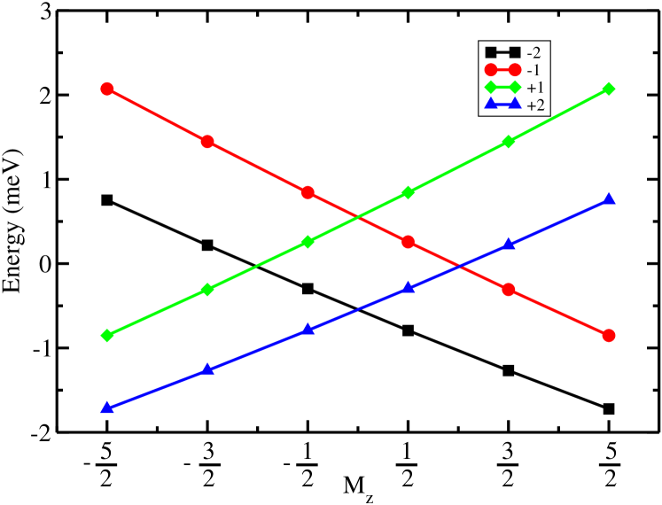
Figure 1: (Color online) Scheme of the energy levels of the quantum dot exciton interacting with 1 Mn when spin-flip terms are neglected.

II.4.2 Wave functions

When spin-flip terms are restored in the Hamiltonian, the $P$ states are no longer eigenstates, but they form a very convenient basis to expand the actual eigenstates of ${\cal H}$, denoted by $|\Psi_{n}\rangle$:

$$|\Psi_{n}\rangle=\sum_{P}\Psi_{n}(P)|P\rangle=\sum_{X,M_{z}}\Psi_{n}(X,M_{z})|X,M_{z}\rangle$$ (43)

In most cases, there is a strong overlap between $\Psi_{n}$ and a single state $|P\rangle$. This is expected for several reasons. First, the single ion in plane anisotropy is probably much smaller than the uniaxial anisotropy, $D\gg E$. Second, the electron-hole exchange, which is the exchange energy in the system, splits the dark and bright levels. Thus, both electron and hole spin flip due to the exchange with the Mn spin is inhibited because they involve coupling between energy split bright and dark excitons. In addition, the electron Mn exchange is smaller than the hole Mn exchange, whose spin-flip part is proportional to the LH-HH mixing and approximately 10 times smaller than the Ising part. In order to quantify the degree of spin mixing of an exact exciton state $\Psi_{n}$, we define the inverse participation ratio:

$$IPZ_{n}\equiv\sum_{P}|\Psi_{n}(P)|^{4}$$ (44)

This quantity gives a measure of the delocalization of the state $\Psi_{n}$ on the space of product states of eq. (41). In the absence of mixing of different $P$ states, we have $IPZ_{n}=1$. In the case of a state equally delocalized in the 24 states of the $P$ space, we would have $\Psi_{n}(P)=\frac{1}{\sqrt{24}}$ and $IPZ_{n}=\frac{1}{24}$.

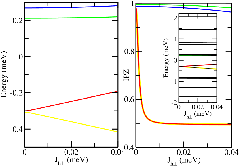
Figure 2: (Color online) Left panel: Evolution of the exciton levels as a function of the LH-HH mixing parameter $J_{h\perp}$. Right panel: Evolution of the IPZ as a function of the LH-HH mixing parameter. The inset presents the evolution of the energy for all the 24 exciton levels.

In figure (2) we plot the evolution of both the energy (left panel) and the $IPZ$ (right panel) as a function of $J_{h\perp}$, the LH-HH mixing parameter, of four states denoted by their dominant component at $J_{h\perp}=0$. For our choice of exchange constants, two of them $|+1,-\frac{3}{2}\rangle$ and $|-2,-\frac{1}{2}\rangle$ are almost degenerate at $J_{h\perp}=0$, which means that the hole-Mn exchange compensates the dark-bright splitting, and couple these states via a hole-Mn spin flip. As a result, their energy levels split linearly as a function of $J_{h\perp}$ and the wave-functions have a large weight on the two product states for finite $J_{h\perp}$. In contrast, the other two levels shown in figure (2), $|+1,-\frac{1}{2}\rangle$ and $|-2,-\frac{3}{2}\rangle$ are not coupled via hole-Mn spin flip. As a result, their energies shift as a function of $J_{h\perp}$ due to coupling to other states, and their IPZ undergoes a minor change, reflecting moderate mixing.

II.4.3 Exchange induced dark-bright mixing

The most conspicuous experimentally observable consequence of the exchange induced mixing, is the transfer of optical weight from the bright to the dark exciton, which results in the observation of more than 6 peaks in the PL. This can be understood as follows. The spin-flip part of the hole-Mn interaction couples the bright exciton $|+1,M_{z}\rangle$ to the dark exciton $|-2,M_{z}+1\rangle$. Thus, a state with dominantly dark character $|-2,M_{z}+1\rangle$ and energy given, to first order, by that of the dark exciton, has a small but finite probability of emitting a photon through its bright component, via a Mn-hole coherent spin-flip. Thus, PL is seen at transition energy of the dark exciton. Reversely, nominally bright excitons loose optical weight due to their coupling to the dark sector. Importantly, the emission of a photon from a dark exciton with dominant Mn spin component $M_{z}$, entails carrier-Mn spin exchange, so that the ground state has $M_{z}\pm 1$.

According to previous theory work Fernandez-Rossier_PRB_2006 the rate for the emission of a circularly polarized photon from the exciton state $\Psi_{n}$ to the ground state $\phi_{m}$ reads:

$$\Gamma^{\pm}_{n,m}=\Gamma_{0}\left|\sum_{M_{z}}\phi_{m}(M_{z})\Psi^{*}_{n}(M_{z},X=\pm 1)\right|^{2}$$ (45)

where

$$\Gamma_{0}\equiv\frac{3\omega^{3}d_{cv}^{2}}{4\pi\epsilon\hbar c^{3}}$$ (46)

is the recombination rate of the bare exciton, $\omega$ is the frequency associated to the energy difference between the exciton state $n$ and the ground state $m$, $c$ is the speed of light, $\epsilon$ is the dielectric constant of the material, $d_{cv}$ is the dipole matrix element. From the experiments, we infer $\Gamma_{0}=$0.5 ns^-1

In the absence of spin-flip terms, the matrix $\Gamma^{\pm}_{n,m}$ would have only non-zero elements for $n=|X=\pm 1,M_{z}\rangle$ states connected to $m=M_{z}$ states. The presence of spin-flip terms in the Hamiltonian enables the recombination from exciton states with dominant dark component. In figure (3) we represent the matrix elements $\Gamma^{\pm}_{n,m}/\Gamma_{0}$ for $j_{eh}=-0.73meV$, $j_{h}=0.36meV$, $j_{e}=-0.09meV$, $j_{h\perp}=0.036meV$, $D=0.01meV$ and $E=0meV$. It is apparent that the recombination rates from the dark states are, at least, 2 times smaller (a and b) than those of the bright states. For $\Gamma_{0}$= 0.4 ns^-1, the lifetime of the dark excitons (a and b) are in the range of 3 ns. Thus, this provides a quite efficient Mn spin relaxation mechanism, provided that a dark exciton is present in the quantum dot.

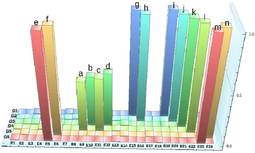
Figure 3: (Color online) Recombination rates of the excitons levels in a Mn doped quantum dot $\Gamma_{i}/\Gamma_{0}$: $a:|+2,+\frac{1}{2}>\rightarrow|+\frac{3}{2}>$, $b:|-2,-\frac{1}{2}>\rightarrow|-\frac{3}{2}>$, $c:|-1,+\frac{3}{2}>\rightarrow|+\frac{3}{2}>$, $d:|+1,-\frac{3}{2}>\rightarrow|-\frac{3}{2}>$, states from e to n are bright excitons. Other states are mainly dark excitons with a small bright component.

The recombination rate matrix, together with the non-equilibrium occupation of the exciton states, $P_{n}$, determines the PL spectrumFernandez-Rossier_PRB_2006 for $\pm$ circular polarization:

$${\cal I}_{\rm PL}^{\pm}(\omega)=\sum_{n,m,}P_{n}\Gamma^{\pm}_{n,m}\delta\left(\hbar\omega-E_{n}-E_{m}\right)$$ (47)

In a typical PL spectrumLe-Gall_PRB_2010 , the dark peaks are, at most, 2 times smaller than the bright peaks. Since $\Gamma^{\pm}_{n,m}$ is at least 2 times smaller for dark states, this implies a larger occupation of the dark states. Thus, we can infer a transfer from the optical ground state to the dark exciton states, via the bright exciton states. This transfer requires an incoherent spin flip of either the electron or hole. Below we show that phonon induced hole-spin relaxation provides the most efficient channel for this bright to dark conversion.

III Mn spin relaxation due to spin-phonon coupling

In this section we discuss the Mn spin relaxation in the absence of excitons. In the absence of carriers and given the fact that Mn-Mn distance is comparable to the dot-dot distance (100 nm for a dot and Mn density of about $10^{10}cm^{-2}$), which makes direct super-exchange negligible, the Mn-phonon coupling should be the dominant, albeit small, Mn spin relaxation mechanism. Transverse phonons induce local rotations of the lattice. Since the crystal field, together with spin orbit coupling, determines the Mn magnetocrystalline anisotropy, the phonon induced lattice rotation Chudnovsky_PRB_2005 acts as a stochastic torque on the Mn spin, resulting in spin relaxation.

The atomic displacement at point $\vec{r}$ in the crystal is expressed in terms of the phonon operators with wave vector $\vec{q}$, polarization mode $\lambda=T1,T2,L$, frequency $\omega_{\lambda}(\vec{q})$ and polarization vector $\vec{e}_{\lambda}(\vec{q})$Cardona-Yu :

$$\vec{u}(\vec{r})=\sum_{\vec{q},\lambda}{\cal U}_{\lambda}(\vec{q})\vec{e}_{\lambda}(\vec{q})\left(b^{\dagger}_{\vec{q},\lambda}+b_{-\vec{q},\lambda}\right)e^{i\vec{q}\cdot\vec{r}}$$ (48)

where

$${\cal U}_{\lambda}(\vec{q})=\sqrt{\frac{\hbar}{2\rho\omega_{\lambda}(\vec{q})V}}$$ (49)

and $V$ and $\rho$ are the volume of the crystal and the mass density respectively. In a zinc-blende structure there are two transverse acoustic (TA) phonon branches and one longitudinal acoustic branch (LA). Following WoodsWoods04 we have:

$$\vec{e}_{TA1}=\frac{1}{qq_{\perp}}\left(q_{x}q_{z},q_{y}q_{z},-q_{\perp}^{2}\right)$$ (50)

$$\vec{e}_{TA2}=\frac{1}{q_{\perp}}\left(q_{y},-q_{x},0\right)$$ (51)

where $q\equiv|\vec{q}|$ and $q_{\perp}=\sqrt{q_{x}^{2}+q_{y}^{2}}$. These vectors satisfy $\vec{q}\cdot\vec{e}_{TAi}=0$, and $\vec{e}_{TAi}\cdot\vec{e}_{TAj}=\delta_{ij}$ The longitudinal mode has $\vec{e}_{LA}=\frac{1}{q}\vec{q}$.

The lattice rotation vector is given by Chudnovsky_PRB_2005

$$\vec{\delta\Phi}(\vec{r})=\vec{\nabla}\times\vec{u}(\vec{r})$$ (52)

so that only the transverse modes contribute. Within this picture, the Mn spin-phonon coupling can be written asChudnovsky_PRB_2005 :

$${\cal V}_{\rm M-ph}=i\left[{\cal H}_{0},\vec{M}\right]\cdot\vec{\delta\Phi}(\vec{r}_{Mn})$$ (53)

Without loss of generality we can set the Mn position as the origin, $\vec{r}_{Mn}=0$. Equation (53) couples the Mn spin to a reservoir of phonons whose non-interacting Hamiltonian is

$${\cal H}_{\rm ph}=\sum_{\vec{q},\lambda}\hbar\omega_{\lambda}(\vec{q})b^{\dagger}_{\vec{q},\lambda}b_{\vec{q},\lambda}$$ (54)

Within the standard system plus reservoir master equation approach, we have derived the scattering rate from a state $n$ to a state $n^{\prime}$, both eigenstates of the single Mn Hamiltonian ${\cal H}_{0}$, due the emission of a phonon. In order to use a general result for that rate (101), derived in the appendix (B), we need to express the spin-phonon coupling (53) using the same notation than in equation (95):

$${\cal V}^{n,n^{\prime}}_{\vec{q},\lambda}=i^{2}{\cal U}_{\lambda}(\vec{q})\vec{f}_{n,n^{\prime}}\cdot\left(\vec{q}\times\vec{e}_{\lambda}(\vec{q})\right)$$ (55)

where

$$\vec{f}_{n,n^{\prime}}\equiv\langle n|\left[{\cal H}_{0},\vec{M}\right]|n^{\prime}\rangle$$ (56)

We compute now the scattering rate due to a single phonon emission assuming 3 dimensional phonons described above. The rate reads:

$$\Gamma_{n\to n^{\prime}}=\frac{|\Delta|^{3}}{12\pi\rho\hbar^{4}c^{5}}(n_{B}(\Delta)+1)\sum_{b,b^{\prime}=x,y,z}f^{b}_{n^{\prime},n}(f^{b^{\prime}}_{n^{\prime},n})^{\ast}$$ (57)

where $c=1.79\textrm{kms}^{-1}$ is the CdTe speed of soundmerle84 , $\rho=5870\text{kgm}^{-3}$ is the mass density of the CdTe unit cellcollins80 and $n_{B}(\Delta)\equiv\frac{1}{e^{\beta|\Delta|}-1}$. The $|\Delta|^{3}$ factor comes from the dependence of the phonon density of states on the energy.

III.1 Mn spin relaxation in the optical ground state

We now discuss the relaxation of the Mn electronic spin due to spin-phonon coupling without an exciton in the quantum dot. According to our experimental resultsLe-Gall_PRL_2009 ; Le-Gall_PRB_2010 , the Mn spin relaxation time in our samples is at least 5$\mu$s.

If we take $E=0$, the transition rate between the excited states $|\phi_{n}\rangle=|M_{z}=+\frac{5}{2}\rangle$ and $|\phi_{n^{\prime}}\rangle=|M_{z}=+\frac{3}{2}\rangle$, via a phonon emission, is given by:

$$\Gamma_{n\to n^{\prime}}=\frac{640|D|^{5}}{3\pi\rho\hbar^{4}c^{5}}(n_{B}(\Delta)+1)$$ (58)

The dependence on $D^{5}$ comes both from the density of states of phonons $\rho\propto\omega^{3}$ and the square of the Mn phonon coupling, which is proportional to the anisotropy, and gives the additional $D^{2}$ factor. Whereas the uniaxial anisotropy of Mn in CdTe quantum wells has been determined by EPR Qazzaz , the actual value for Mn in quantum dots is not known and can not be measured directly from single exciton spectroscopy of neutral dots. Therefore, in figure (4) we plot the lifetime for the transition of the Mn spin from $\frac{5}{2}$ to $\frac{3}{2}$, due to a phonon emission, as a function of $D$. We take $D$ in a range around the value reported for CdTe:Mn epilayers, $D=12\mu$eV Qazzaz . We find that the spin lifetime of Mn in the optical ground state can be very large. Even for $D=20\mu eV$ the Mn spin lifetime is in the range of 0.1 seconds, well above the lower limit for the Mn spin relaxation reported experimentallyLe-Gall_PRL_2009 ; Le-Gall_PRB_2010 . Whereas we can not rule out completely that the Mn spin lifetimes that long, there are other spin relaxation mechanisms that might be more efficient that the Mn-phonon coupling considered above, like the coupling of the Mn electronic spin to nuclear spins of Mn and the host atomsLe-Gall_PRL_2009 .

Since part of the $\Delta^{5}$ scaling arises from the $\omega^{3}$ scaling of the phonon density of states, we have explored the possibility that phonons localized in the wetting layer could be more efficient in relaxing the Mn spin. For that matter we have considered a toy model of two dimensional phonons confined in a slab of thickness $L=2\,nm$. The resulting Mn spin relaxation rate for those reads:

$$\Gamma_{n\to n^{\prime}}=\frac{\Delta^{2}}{16\hbar^{3}c^{4}\rho W}(n_{B}(\Delta)+1)\sum_{b,b^{\prime}=x,y,z}A_{b,b^{\prime}}f^{b}_{n^{\prime},n}(f^{b^{\prime}}_{n^{\prime},n})^{\ast}$$ (59)

where W is the width of the sample and A is a diagonal matrix with $A_{xx}=1$, $A_{yy}=1$, $A_{zz}=2$.

In figure (4) we plot the associated spin lifetime in this case, taking $W=2nm$ and show how it is at least 100 shorter than for 3D phonons, but still we would have $T_{1}\simeq 1$ ms for $D=20\mu$eV.

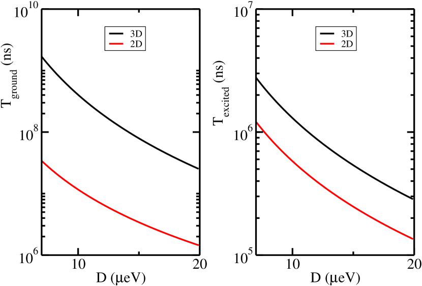
Figure 4: (Color online) Left panel: Lifetime of the (+$\frac{5}{2}$ to +$\frac{3}{2}$) transition in the optical ground state at zero field as a function of the magnetic anisotropy energy splitting $D$. Right panel: Lifetime of the same transition in the presence of a $+1$ exciton for different values of $D$. The rates are calculated for a 3 dimensional (3D) and a 2 dimensional (2D) density of states of acoustic phonons.

III.2 Mn spin relaxation in the presence of an exciton

Here we discuss how the Mn spin relaxation due to Mn-phonon coupling is modified when an exciton is interacting with the Mn. The Mn-phonon coupling is still given by Hamiltonian (53), with ${\cal H}_{0}$ given by eq. (1). We assume that the only effect of the exciton on the Mn is to change the energy spectrum and mix the spin wave-functions, giving rise to larger spin relaxation rates, due to the larger exchange-induced energy splittings.

In the presence of the exciton, the Mn-phonon coupling results in transitions between different exciton-Mn spin states, $n$ and $n^{\prime}$. As we did in the case of the Mn without excitons, we need to express the spin-phonon coupling (53) using the same notation than in equation (95).

For that matter we define the matrix elements

$$\vec{F}_{n,n^{\prime}}\equiv\langle\Psi_{n}|\left[{\cal H}_{0},\vec{M}\right]|\Psi_{n}^{\prime}\rangle=$$

$$\sum_{X,M_{z},M_{z}^{\prime}}\Psi_{n}(X,M)^{*}\Psi_{n}(X,M^{\prime})^{*}\vec{f}_{M,M^{\prime}}$$ (60)

where

$$\vec{f}_{M,M^{\prime}}\equiv\langle M|\left[{\cal H}_{0},\vec{M}\right]|M^{\prime}\rangle$$ (61)

$M$ and $M^{\prime}$ stand for eigenstates of the Mn spin operator $M_{z}$. Thus, in the exciton-Mn spin states basis, the Mn-phonon coupling reads:

$${\cal V}^{n,n^{\prime}}_{\vec{q},\lambda}=i^{2}{\cal U}_{\lambda}(\vec{q})\vec{F}_{n,n^{\prime}}(M)\cdot\left(\vec{q}\times\vec{e}_{\lambda}(\vec{q})\right)$$ (62)

Notice how if we neglect the spin mixing of the exciton states we have $\vec{F}_{n,n^{\prime}}=\vec{f}_{M,M^{\prime}}$ and the only difference in the scattering rates arises from the larger energy splittings in the presence of the exciton.

Using the equation (101) for the phonon induced spin relaxation rate, and in analogy with equation (57) we write:

$$\Gamma_{n\to n^{\prime}}=\frac{|\Delta|^{3}}{12\pi\rho\hbar^{4}c^{5}}(n_{B}(\Delta)+1)\sum_{b,b^{\prime}=x,y,z}F^{b}_{n,n^{\prime}}(F^{b^{\prime}}_{n,n^{\prime}})^{\ast}$$ (63)

In figure (4) we see how Mn-phonon spin relaxation is much faster in the presence of the exciton. Ignoring the difference arising from the spin mixing, we can write the ratio of the rates as:

$$\frac{\Gamma_{n\to n^{\prime}}(X)}{\Gamma_{n\to n^{\prime}}(G)}=\left(\frac{\Delta_{X}}{\Delta_{G}}\right)^{3}$$ (64)

The energy splitting associated to the $\frac{5}{2}$ to $\frac{3}{2}$ spin flip in the ground state is $4D$. In the presence of the exciton the energy splitting of the same transition would be $4D+j_{h}-j_{e}$. If we take $D=12\mu$eV, $j_{h}=360\mu$eV and $j_{e}=-90\mu$eV the ratio yields $\approx 10^{3}$. From the experimental side we know that $T_{1G}>5\mu s$ and, in the presence of the exciton $T_{1}\simeq 50ns$. Thus, the ratio could be accounted for by this mechanism. However, in order to have $T_{1G}=5\mu$s we would need to assume an unrealistically large value for $D$. Thus, we think that another spin relaxation mechanism must be operative in the system when the exciton is in the dot which makes it possible to control the spin of the Mn in a time scale of 50 ns. In the next sections we discuss the hole spin relaxation due to phonons as the mechanism that, combined with Mn-carrier exchange, yields a quick Mn spin relaxation in the presence of the exciton.

IV Hole spin relaxation in non magnetic dots

IV.1 Hole-phonon coupling

We now consider the relaxation of the hole spin due to hole-phonon coupling. We consider first the case of undoped quantum dots. The coupling of the spin of the hole to phonons can be understood extending the Bir Pikus Hamiltonian to the case of inhomogeneous strain associated to lattice vibrations:

$$\epsilon_{ij}(\vec{r})\equiv\frac{1}{2}\left(\frac{\partial u_{i}}{\partial r_{j}}+\frac{\partial u_{j}}{\partial r_{i}}\right)$$ (65)

It is convenient to write the strain tensor field as:

$$\epsilon_{ij}(\vec{r})=\sum_{\vec{q}}e^{i\vec{q}\cdot\vec{r}}\epsilon_{ij}(\vec{q})$$ (66)

so that we write:

$$\epsilon_{ij}(\vec{q})=\frac{1}{2}\sum_{\lambda}{\cal U}_{\lambda}(\vec{q})\left(b^{\dagger}_{\vec{q},\lambda}+b_{-\vec{q},\lambda}\right)\left(q_{j}e^{i}_{\lambda}(\vec{q})+q_{i}e^{j}_{\lambda}(\vec{q})\right)$$ (67)

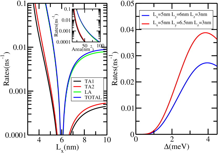
Figure 5: (Color online) Left panel: Hole spin-flip rate as a function of the dot size and shape. $L_{y}$ is fixed at 6nm, scaning of $L_{x}$ change the LH-HH mixing. In the inset the ratio $L_{y}/L_{x}$ is fixed at 1.2 so the shape of the dot are fixed, only the size of the dot changes. One can see that the hole spin-flip rate is a size sensitive quantum quantity, the rate is a semi-exponential function of the size of the dot. Right panel: Hole spin-flip rate as a function of the energy splitting for two different values of the quantum dot anisotropy, ie LH-HH mixing.

We consider the coupling of the ground state doublet, formed by states $\Uparrow$ and $\Downarrow$, to the phonon reservoir Roszak_PRB_2007 . The effective hole-phonon Hamiltonian is obtained by projecting the BP Hamiltonian onto this subspace:

$${\cal V}_{\rm h-phonon}=\sum_{ij,\vec{q}\sigma_{h},\sigma_{h}^{\prime}}I^{\sigma_{h},\sigma_{h}^{\prime}}_{ij}(\vec{q})|\sigma_{h}\rangle\langle\sigma_{h}^{\prime}|\epsilon_{ij}(\vec{q})$$ (68)

Here $|\sigma_{h}\rangle$ denotes the quantum dot state defined in eq. (23) and the coupling constant reads

$$I^{\sigma_{h},\sigma_{h}^{\prime}}_{ij}(\vec{q})\equiv\sum_{j_{z},j_{z}^{\prime}}V_{ij}{\cal C}_{h}^{*}(j_{z}){\cal C}_{h^{\prime}}(j_{z}^{\prime})\langle j_{z}|J_{i}J_{j}|j_{z}^{\prime}\rangle I_{\vec{q}}$$ (69)

where $I_{\vec{q}}=\int|\psi_{0}(\vec{r})|^{2}e^{i\vec{q}\cdot\vec{r}}d\vec{r}$. Hamiltonian (68) shows how the absorption or emission of a phonon can induce a transition between the two quantum dot hole states, $\Uparrow$ and $\Downarrow$.

We now calculate the time scale for the spin relaxation of a single hole in a non magnetic dot under the influence of an applied magnetic field so that the hole ground state doublet is split in energy. In order to compute the transition rate for decay of the hole from the excited to the ground state we use again the general equation (101). For that matter, we express the hole-spin coupling (68) as:

$${\cal V}_{\rm h-phonon}=\sum_{\vec{q},\lambda\sigma_{h},\sigma_{h}^{\prime}}{\cal V}^{\sigma_{h},\sigma_{h}^{\prime}}_{\vec{q},\lambda}|\sigma_{h}\rangle\langle\sigma_{h}^{\prime}|\left(b_{\lambda q}^{\dagger}+b_{\lambda,-q}\right)$$ (70)

where

$${\cal V}^{\sigma_{h},\sigma_{h}^{\prime}}_{\vec{q},\lambda}=\frac{i}{2}\sum_{i,j}I^{\sigma_{h},\sigma_{h}^{\prime}}_{ij}(\vec{q}){\cal U}_{\lambda}(\vec{q})\left(q_{i}e^{j}_{\lambda}(\vec{q})+q_{j}e^{i}_{\lambda}(\vec{q})\right)$$ (71)

IV.2 Calculation of hole spin-flip rates with simple model

In order to illustrate the physics of the phonon-driven hole spin relaxation we consider the case of a single hole in a non-magnetic dot under the influence of an applied magnetic field. For that matter, we compute the Hamiltonian (71) using the wave functions from the simple model of confined holes defined in eq. (16). We focus on the non-diagonal terms in the hole spin index, i.e., the terms that result in scattering form $\Uparrow$ to $\Downarrow$ due to phonon emission.

Importantly, the BP Hamiltonian couples hole states that differ in, at most, two units of $J_{z}$. Thus, in the absence of LH-HH mixing, the BP Hamiltonian does not couple directly the $\Uparrow$ and $\Downarrow$ states. Transitions between $\Uparrow$ and $\Downarrow$ states, as defined in eq. (23), are only possible, through one phonon processes, through the $\epsilon_{yz}(J_{y}J_{z}+J_{z}J_{y})$ and $\epsilon_{zx}(J_{z}J_{x}+J_{x}J_{z})$ terms in the Hamiltonian. After a straightforward calculation we obtain:

$${\cal V}^{\Uparrow,\Downarrow}_{\vec{q},\lambda}=\frac{i}{2}\sqrt{3}dSin\left(\frac{\theta_{1}-\theta_{2}}{2}\right)\left(\epsilon_{yz}(\vec{q})-i\epsilon_{zx}(\vec{q})\right)$$ (72)

The important role played by the $LH-HH$ mixing $\theta_{1,2}$ is apparent. Using equation (101) it is quite straightforward to compute the rate for the 3 phonon branches. They are all proportional to

$$\Gamma^{0}_{\Uparrow\rightarrow\Downarrow}=\frac{1}{18\pi}D_{u^{\prime}}^{2}Sin^{2}\left(\frac{\theta_{1}-\theta_{2}}{2}\right)\frac{\Delta^{3}}{\rho\hbar^{4}c^{5}}$$ (73)

with coefficients $\frac{7}{5}$, $1$ and $\frac{8}{5}$ for the TA1, TA2 and L modes respectively. Here, $D_{u^{\prime}}$ stands for the deformation potential of Kleiner-Rothkleiner , following reference willatzen, , $D_{u^{\prime}}=-\frac{3\sqrt{3}d}{2}$. $\rho$ for the mass density of CdTe, $c$ for its transverse speed of sound, and $\Delta$ for the energy splitting between the $\Uparrow$ and $\Downarrow$ states, which is proportional to the external magnetic field $B$. In figure (5) we plot the rates $\Gamma_{TA1},\Gamma_{TA2},\Gamma_{L}$, as well as their sum as function of the dot size (left panel) and as a function of the energy splitting between the initial and final hole state, $\Delta$ (right panel). We see how hole spin relaxation rates can be in the range of $\Gamma\simeq 1/(40ns)$.

The results of figure (5) suggest that for sufficiently high $\Delta$, as those provided by the Mn-hole exchange, the hole spin can relax in a time scale of 30$ns$. These numbers are in the same range than those obtained by Woods et al Woods04 . As we discuss in the next section, these spin flips, together with Mn-carrier exchange, can also induce Mn spin relaxation in a time scale much shorter than the one due to Mn-phonon coupling only.

Importantly, the rate is finite only if $\theta_{1}-\theta_{2}\neq 0$, which is the case in the presence of an applied magnetic field. This indicates that, within the simple model of eq. (16), the non-diagonal terms in the hole-phonon Hamiltonian (68) vanishes identically. This is not a general feature of (68), but rather an particular property of the simple model (16). In particular, the non-diagonal term in (16) is non-zero at zero field as soon as the ($+\frac{3}{2},-\frac{1}{2}$) states have also some weight on the $+\frac{1}{2}$ components, which happens both when a more realistic model for confinement is used or when homogeneous strain components $e_{yz}$ and $e_{zx}$ are included.

V Spin relaxation in magnetic dots due to hole-phonon coupling

The results of the previous sections indicate that, because of their coupling to phonons, the hole spin lifetime in a non-magnetic dot is much shorter than the Mn spin lifetime. Here we explore the consequences of this phonon-driven hole spin relaxation for the single exciton states in a dot doped with one magnetic atom. The leading process results in a Mn spin conserving decay from the bright exciton to the dark exciton state, via hole-spin flip in a time scale in the 10 ns range. Combined with the optical recombination of the dark state, made possible via Mn-hole or Mn-electron spin flip, provide a pathway for exciton induced Mn spin relaxation in a time scale under 100 ns, as observed experimentally Le-Gall_PRL_2009 ; Goryca_PRL_2009 ; Le-Gall_PRB_2010 .

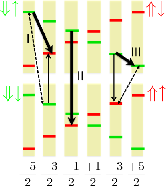
Figure 6: (Color online) Scheme of the Mn spin flip channels due to the combined action of hole-phonon coupling and carrier-Mn exchange.

We also explore the scattering between two bright states enabled by the combination of phonon induced hole spin relaxation and Mn-carrier exchange. The lifetimes of these processes is in the range of $10^{3}$ ns and higher, and therefore they are probably not determinant for the optical orientation of the Mn spin in the sub-microsecond scale.

V.1 Exciton-phonon coupling in magnetic dots

The Hamiltonian that couples the exciton states $\Psi_{n}$ to the phonons is derived by projecting the hole-phonon coupling Hamiltonian (68) onto the exciton states (43) . The result reads:

$${\cal V}_{\rm X-phon}=\sum_{n,n^{\prime}\vec{q}\lambda}|\Psi_{n}\rangle\langle\Psi_{n^{\prime}}|{\cal V}^{n,n^{\prime}}_{\vec{q},\lambda}\left(b_{\lambda q}^{\dagger}+b_{\lambda,-q}\right)$$ (74)

where

$${\cal V}^{n,n^{\prime}}_{\vec{q},\lambda}=\sum_{M_{z},\sigma_{e},\sigma_{h},\sigma_{h}^{\prime}}{\cal V}^{\sigma_{h},\sigma_{h}^{\prime}}_{\vec{q},\lambda}\Psi_{n}(M_{z},X)\Psi^{*}_{n^{\prime}}(M_{z},X^{\prime})$$ (75)

where $X=(\sigma_{e},\sigma_{h})$ and $X^{\prime}=(\sigma_{e},\sigma_{h}^{\prime})$ (same electron spin) and ${\cal V}^{\sigma_{h},\sigma_{h}^{\prime}}_{\vec{q},\lambda}$ is given by equation (71).

V.2 Qualitative description of the spin relaxation processes

In order to describe qualitatively the variety of different processes accounted for by Hamiltonian (74) it is convenient to consider an initial state $\psi_{n}$ as a linear combination of a dominant component $|M\rangle|\downarrow\rangle_{e}|\Uparrow\rangle_{h}$ plus a minor contribution of two dark components, which arise from the coherent exchange of the Mn with either the electron or the hole:

$$|\psi_{n}\rangle = |M\rangle|\downarrow\rangle_{e}|\Uparrow\rangle_{h}+$$

$$+ \epsilon_{e}|M-1\rangle|\uparrow\rangle_{e}|\Uparrow\rangle_{h}+\epsilon_{h}|M+1\rangle|\downarrow\rangle_{e}|\Downarrow\rangle_{h}$$ (76)

where $\epsilon_{e}\propto j_{e}/j_{eh}$ and $\epsilon_{h}\propto j_{h}/j_{eh}$ are small dimensionless coefficients that can be obtained doing perturbation theory.

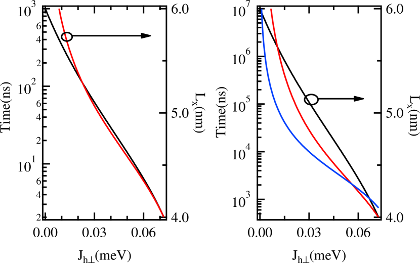
Figure 7: (Color online) Calculated rates for the transitions between exciton states in a Mn-doped quantum dot due to hole-phonon coupling. Left panel, red line, transition from $|-1,-\frac{5}{2}>$ to $|+2,-\frac{5}{2}>$, Right panel, red line, transition from$|-1,-\frac{5}{2}>$ to $|-2,-\frac{1}{2}>$. blue line, transition from $|-1,-\frac{5}{2}>$ to $|+1,-\frac{3}{2}>$. L_y is fixed at 6nm and scanning L_x changes the LH-HH mixing parameter J_h⟂.

Depending on the elementary process that takes place, there are several possible final states:

1. Hole spin relaxation. In this case the final state would be dominantly a dark exciton whose wave function read:

   $$|\psi_{n^{\prime}}\rangle = |M\rangle|\downarrow\rangle_{e}|\Downarrow\rangle_{h}+O(\epsilon)$$ (77)

   and the scattering rate $\Gamma_{0}$ would be proportional to $|I^{\Uparrow,\Downarrow}|^{2}$. This is process II in figure (6).

2. Hole spin relaxation plus coherent hole-Mn spin flip. This is process III in figure (6) This can be realized through 2 dominant channels. An incoherent hole spin flip will couple the dominant component of the initial state, $|M\rangle|~{}\downarrow\rangle_{e}|\Uparrow\rangle_{h}$ with a secondary component $|M\rangle|\downarrow\rangle_{e}|\Downarrow\rangle_{h}$ of the final state

   $$|\psi_{n^{\prime}}\rangle = |M-1\rangle|\downarrow\rangle_{e}|\Uparrow\rangle_{h}+$$

   $$+ \epsilon_{h}|M\rangle|\downarrow\rangle_{e}|\Downarrow\rangle_{h}+O(\epsilon_{e})$$ (78)

   In this case the final state is a bright exciton in the same branch $+1$ than the initial state but the Mn component goes from $M$ to $M-1$.

   The second channel comes from the hole spin flip of the minority dark component of the initial state, $\epsilon_{h}|M+1\rangle|\downarrow\rangle_{e}|\Downarrow\rangle_{h}$ which decays into the majority component of the final state

   $$|\psi_{n^{\prime}}\rangle = |M+1\rangle|\downarrow\rangle_{e}|\Uparrow\rangle_{h}+O(\epsilon_{e,h})$$ (79)

   Thus, in this second case a hole spin flips due to phonons, plus a coherent Mn-electron spin flip connect the $X=+1,M$ initial state to the $X=-1,M+1$ state. Thus, both the initial and final state in this process are the same than in the first channel, the rates for each would be proportional to $\epsilon_{h}^{2}\Gamma_{0}$, but the decay pathways are different, and interferences are expected.

3. Hole spin relaxation plus coherent electron-Mn spin flip. This is process I in figure (6) As in the previous case, there are two channels for this type of process. In the first channel, the majority component of the initial state decays into a final state given by:

   $$|\psi_{n^{\prime}}\rangle = |M-1\rangle|\uparrow\rangle_{e}|\Downarrow\rangle_{h}+\epsilon_{e}^{\prime}|M\rangle|\downarrow\rangle_{e}|\Downarrow\rangle_{h}$$ (80)

   The incoherent hole spin flip connects the initial state (76) to the final state (80) through the minority component $|M\rangle|\downarrow\rangle_{e}|\Downarrow\rangle_{h}$ of the later.

   The second channel comes from the hole spin flip of the minority dark component of the initial state, $\epsilon_{e}|M-1\rangle|\uparrow\rangle_{e}|\Uparrow\rangle_{h}$ which decays into the majority component of the final state

   $$|\psi_{n^{\prime}}\rangle = |M-1\rangle|\uparrow\rangle_{e}|\Downarrow\rangle_{h}+O(\epsilon_{e,h})$$ (81)

   Thus, a hole spin flips due the phonon, plus a coherent Mn-electron spin flip connect the $X=+1,M$ initial state to the $X=-1,M-1$ state. The scattering rate of these two process scales as $\epsilon_{e}^{2}\Gamma_{0}$

V.3 Calculation of the relaxation rates

In order to implement equations (74,75) to compute scattering rates, we use the single particle basis for the holes done with equations (16) which leads, at finite magnetic field to the matrix element (72) that would be incorporated into equations (75) to compute the rates using equation (101). As discussed above, a zero field model (16) yields a zero spin-flip matrix element in equation (72). This is a feature of the simple hole model rather than an intrinsic property of the system. Thus, for the sake of simplicity, we compute the rates between exciton states by computing the matrix element (72) as if there was a magnetic field that yields the energy splitting between the initial and final exciton states equal to the splitting produced by the exchange interaction with the Mn spin.

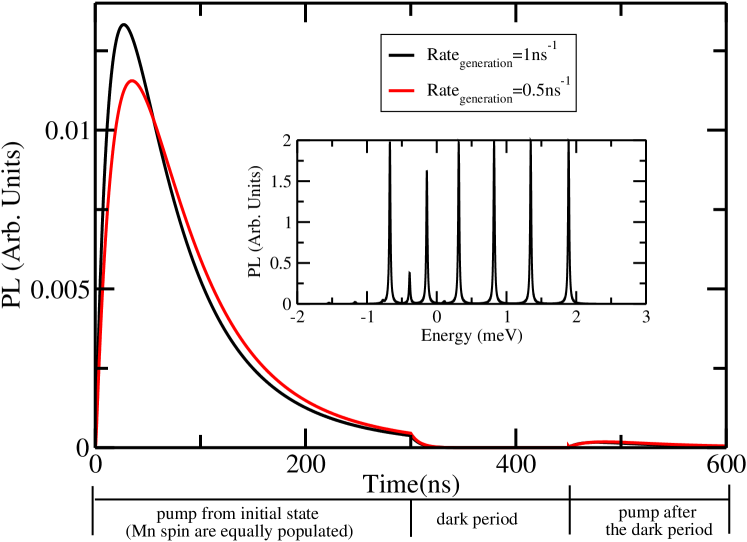
Figure 8: (Color online) Simulation of PL intensity from state ($X=+1$,$M_{z}=-\frac{5}{2}$) under the influence of a driving laser pumping the system resonantly from optical ground state $M_{z}=-\frac{5}{2}$ to the excited state ($X=-1$, $M_{z}=-\frac{5}{2}$) for two laser intensities. The inset is the PL spectrum assuming all the states are equally populated. In the calculation, the quantum dot anisotropy (L_x=5nm and L_y=6nm) controls the LH-HH mixing. The other parameters are discussed in the text.

In the calculation of the rates we perform an additional approximation: we only consider spin-flip terms in equation (75) and we do exclude spin-conserving terms. The results for transition rates from the state $n$ with dominant ($-1,-\frac{5}{2}$) to 3 possible final states with dominant components ($+2,-\frac{5}{2}$), ($-2,-\frac{1}{2}$) and ($+1,-\frac{3}{2}$) as a function of the spin-flip Mn hole exchange $J_{h\perp}$, are shown in figure (7). The transition to the ($+2,-\frac{5}{2}$), which only involves the irreversible spin flip of the hole via a phonon emission is the dominant process and has a lifetime of 30 ns. The transition to the ($+1,-\frac{3}{2}$) state requires both the hole spin flip and the Mn-hole spin flip and it is 3 orders of magnitude less efficient.

Thus, these calculations indicate that the most likely mechanism for Mn spin orientation in the presence of an exciton combines a rapid bright-to dark conversion, produced by phonon induced hole spin flip, and a dark to ground transition, enabled by Mn-carrier spin exchange and radiative recombination.

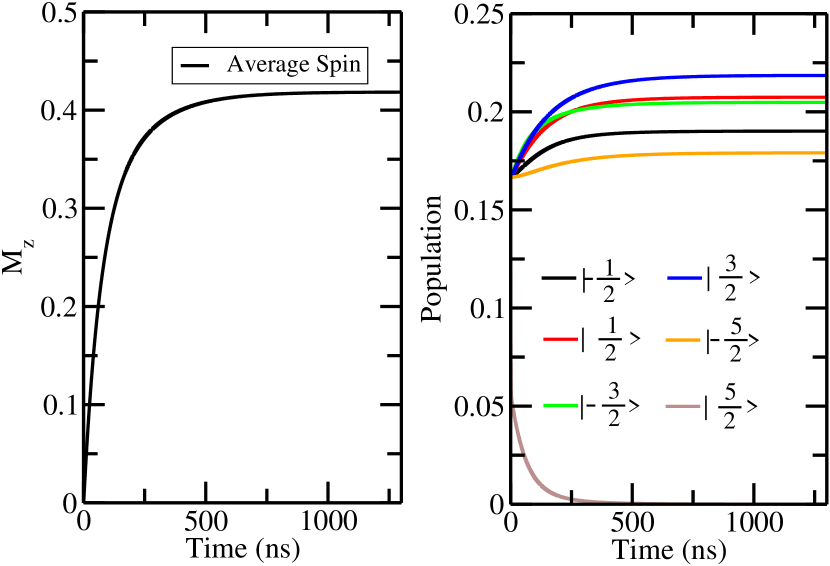
Figure 9: (Color online) Left panel: average magnetization and right panel: occupation of the different spin states under optical pumping of the state ($X=-1$, $M_{z}=-\frac{5}{2}$). Parameters are the same as for the calculation presented in figure (8).

VI Laser driven spin dynamics

VI.1 Summary of scattering mechanisms and master equation

The spin dynamics of a single Mn atom in a laser driven quantum dot is described in terms of the 24 exciton states $\Psi_{n}$ and the 6 ground states $\phi_{m}$. In the previous sections we have calculated the scattering rates of these states. They can be summarized as follows:

1. Transitions from the $\Psi_{n}$ to the $\phi_{m}$, via photon emission (eq. (45)). In the case of bright excitons, this process is the quickest of all, with a typical lifetime of 0.3 ns. In the case of dark excitons the lifetime depends on the bright/dark mixing, which is both level and dot dependent. Dark lifetime ranges from twice the one of bright excitons to 1000 times larger, ie, between 1 and 300 nanoseconds. In any event, dark recombination involves a Mn spin flip.

2. Transitions between different $\phi_{m}$ states, due to Mn spin phonon coupling (eq. (57)). The lifetimes of these transitions are, at least, 1ms (see right panel of figure 4).

3. Transitions between different exciton states $\Psi_{n}$ that flip the spin of the Mn only, due to Mn-phonon coupling (eq. (63). The lifetimes of these transitions are, at least, 0.1ms (see left panel figure 4).

4. Transitions between exciton states due to hole-phonon coupling (eq. (74). The bright to dark transition is the quickest process with a lifetime of about 30ns (see figure 7). Bright to bright transitions, combining hole-phonon and Mn-carrier interactions, have lifetimes in the 10 $\mu s$ range.

In addition to these dissipative scattering processes, we have to consider driving effect of the laser field, described in the semiclassical approximation. All things considered, we arrive to a master equation that describes the evolution of the occupations $p_{N}$, where $N=(n,m)$ includes states both with and without exciton in the dot. The master equation reads:

$$\frac{dp_{N}}{dt}=\sum_{N^{\prime}}\Gamma_{N^{\prime}\rightarrow N}p_{N^{\prime}}-\sum_{N^{\prime}}\Gamma_{N\rightarrow N^{\prime}}p_{N}$$ (82)

Eq. (82) is a system of 36 coupled differential equations that we solve by numerical iteration, starting from a thermal distribution for the initial occupation $p_{N}$. Since the temperature is larger than the energy splitting in the ground state, but much smaller than the band gap, at $t=0$ we have the six ground states with similar occupation $P_{m}\simeq 1/6$, $P_{n}\simeq 0$. As a result, the average magnetization, defined as:

$$\langle M_{z}\rangle=\sum_{m}p_{m}\langle\phi_{m}|M_{z}|\phi_{m}\rangle$$ (83)

is zero, at zero magnetic field, as expected.

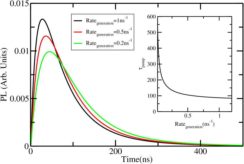
Figure 10: (Color online) Evolution of Mn spin orientation efficiency as a function of the laser power. The pumping is detected in the PL intensity from state ($X=+1$,$M_{z}=-\frac{5}{2}$) under the influence of a driving laser pumping the system from optical ground state $M_{z}=-\frac{5}{2}$ to the excited state ($X=-1$, $M_{z}=-\frac{5}{2}$). The inset presents the laser power dependence of $\tau_{pump}$, from where we can see that the efficiency of the pumping gets higher with the increasing of the laser power.

VI.2 Optical Mn spin orientation

Under the action of the laser, the exciton states become populated and, under the adequate pumping conditions, the average Mn magnetization $\langle M_{z}\rangle$ acquires a non-zero value. This transfer of angular momentum, known as optical Mn spin orientation has been observed experimentally Le-Gall_PRL_2009 and predicted theoreticallyGovorov05 . It results from a decrease of the Mn spin lifetime in the presence of the exciton in the dot. In that circumstance, the laser transfer population from the $M_{z}$ state to the $X,M_{z}$ state. The enhanced relaxation transfers population from $X,M_{z}$ to $X,M_{z}^{\prime}$ and the recombination to $M_{z}^{\prime}$ state. Thus, if the laser is resonant with a single $M_{z}$ to $X,M_{z}$ transition, the $M_{z}$ state is depleted, which results in a decrease of the PL coming both from the $X,M_{z}$ and the $-X,M_{z}$ transitions.

Quantity	Symbol	Value
Hole-Mn exchange	$j_{h}$	0.31 meV
Electron-Mn exchange	$j_{e}$	-0.09 meV
Electron-Hole	$j_{eh}$	-0.73 meV
Uniaxial Anisotropy	$D$	10 $\mu eV$
In plane Anisotropy	$E$	0
Quantum dot width	$L_{y}$	6nm
Quantum dot width	$L_{x}$	5nm
Quantum dot height	$L_{z}$	3nm

Table 1: Parameters used in the simulation of the resonant PL observed in the time resolved optical pumping experiments.

In figure (8) we show the result of our simulations for a dot at thermal equilibrium ($k_{B}T=4$K) at $t=0$ which is pumped with a laser pulse resonant with the $X=-1,M_{z}=-\frac{5}{2}$ transition, which is the high energy one, since the hole is parallel to Mn spin. The laser pulse has a duration of 300 nanoseconds, so that the spectral broadening is negligible. In the upper panel we plot the PL coming from the counter-polarized transition, $X=+1,M_{z}=-\frac{5}{2}$, which has lower energy and can be detected without interference with the laser, for two different pumping power intensity. It is apparent that after a rise of the PL in a time scale of 8 ns, corresponding the spin relaxation of the exciton spin from $X=-1$ to $X=+1$, the PL signal is depleted. The origin of the depletion is seen in figure (9). The occupation of the $M_{z}=-\frac{5}{2}$ spin state in the ground reduced down to zero, in benefit of the other Mn spin states.

Accordingly, the average magnetization becomes finite. Thus, net angular momentum is transferred from the laser to the Mn spin. The transfer takes place through Mn spin relaxation enabled in the presence of the exciton. As discussed above, the most efficient mechanism combines hole-spin relaxation due to phonons combined with dark-bright mixing, which involves a Mn spin flip.

Interestingly, the fact that in the steady state several Mn spin states are occupied, including the higher energy ones, is compatible with a picture in which the Mn spin is precessing. Thus, a steady supply of spin-polarized excitons in the dot would result in the precession of the Mn spin, a scenario similar to that of current drive spin-torque oscillatorsKiselev03 . Further work necessary to confirm this scenario is outside the scope of this paper.

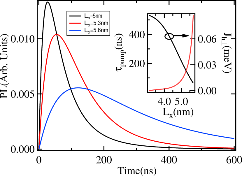
Figure 11: (Color online) Evolution of Mn spin orientation efficiency as a function of the valence band mixing controlled by the anisotropy of the confinement potentiel (L_y=13nm, variable L_x). The pumping is detected in the PL intensity from state ($X=+1$,$M_{z}=-\frac{5}{2}$) under the influence of a driving laser pumping the system from optical ground state $M_{z}=-\frac{5}{2}$ to the excited state ($X=-1$, $M_{z}=-\frac{5}{2}$). The inset shows the evolution of $\tau_{pump}$ with L_x and J_h⟂. The exciton generation rate is fixed at 1 ns^-1.

The efficiency of the process increases with the laser power, as shown in figure (10). We define the spin orientation time $\tau_{pump}$ as the time at which the PL of the counter polarized transition is half the maximum. We can see that, as expected, $\tau_{pump}$ is a decreasing function of the laser power. A pumping time $\tau_{pump}\simeq$90ns is obtained with a generation rate of about 1ns^-1. The amplitude of the valence band mixing, controlled by the anisotropy of the confinement potential or the in-plane strain distribution, is the main quantum dot parameter controlling the efficiency of the optical pumping. As presented in figure (11), decreasing the quantum dot anisotropy, i.e., decreasing the LH-HH mixing parameter J_h⟂, produces a rapid increase of $\tau_{pump}$ (inset of figure (11). This is a direct consequence of the reduction of the phonon induced hole spin flip.

VII Summary and conclusions

We have studied the spin dynamics of a single Mn atom in a CdTe quantum dot excited by a laser that drives the transition between the 6 optical ground states, associated to the $2S+1$ states of the Mn spin $S=\frac{5}{2}$, and the 24 single exciton states, corresponding to $X=\pm 1,\pm 2$ states interacting with the Mn spin. The main goal is to have a microscopic theory for the Mn spin relaxation mechanisms that makes it possible to produce laser induced Mn spin orientation in a time scale of less than 100 ns. Le-Gall_PRL_2009 ; Goryca_PRL_2009 ; Le-Gall_PRB_2010 For that matter, we need to describe how the Mn and the quantum dot exciton affect each other.

In section (II) we describe the different terms in the Mn spin Hamiltonian, including exchange with the 0-dimensional exciton. The symmetry of the exchange interaction depends on the spin properties of the carriers, which in the case of holes are strongly affected by the interplay of confinement, strain and spin orbit coupling. In section (II) we also use a model for holesdot-holes ; Fernandez-Rossier_PRB_2006 ; Kuhn09 in quantum dots, which permits to obtain analytical expressions for the wave functions of the holes, the hole-Mn exchange, in terms of the dimensions of the dot and the Kohh-Luttinger Hamiltonian.

In section (III) we study the dissipative dynamics of the Mn spin due to its coupling to phonons, both with and without excitons in the dot. The Mn spin-phonon coupling arises from the time dependent stochastic fluctuations of the crystal field and thereby of the single ion magnetic anisotropy, induced by the phonon field. Whereas the Mn spin relaxation is accelerated by 2 or 3 orders of magnitude in the presence of the exciton, the efficiency of this mechanism is too low to account for the optical orientation of the Mn spin reported experimentallyLe-Gall_PRL_2009 ; Goryca_PRL_2009 ; Le-Gall_PRB_2010 . The small Mn spin-phonon coupling comes from the small magnetic anisotropy of Mn as a substituional impurity in CdTe.

In section (IV) we describe the interaction between the hole spin and the phonons in non-magnetic dots. Using the simple analytical model for the holes presented in section II we obtain analytical formulas for the hole spin relaxation. We find that hole spin lifetime can be in the range of 30 ns for a hole spin splitting as large as that provided by the hole-Mn coupling. Thus, we expect that bright excitons will relax into dark excitons via hole-spin relaxation. This provides a microscopic mechanism to the scenario for Mn spin relaxation proposed by Cywinski Cywinski10 : bright excitons relax into dark excitons, via carrier spin relaxation, and the joint process of Mn-carrier spin exchange couples the dark excitons to the bright excitons, resulting in PL from dark states which implies Mn spin relaxation in a time scale of a few nanoseconds. This scenario is confirmed by calculations presented in section V. Finally, in section VI we present the master equation that governs the dynamics of the 30 states of the dot, we solve it numerically and we model the optical Mn spin orientation reported experimentally.

Our main conclusions are:

• Mn spin-phonon spin relaxation is presumably too weak to account for Mn spin dynamics in the presence of the exciton

• The Mn spin orientation is possible in a time scale of one hundred nanoseconds via a combination of phonon-induced hole spin relaxation and the subsequent recombination of the dark exciton enabled by spin-flip exchange of the Mn and the carrier

• The critical property that governs the hole-Mn exchange and the hole spin relaxation is the mixing between light and heavy holes, which depends both on the shape of the dot and on strain.

• Our microscopic model permits to account for the optically induced Mn spin orientation.

Future work should address how the coupling of the electronic Mn spin to the nuclear spin modifies our results. This probably plays a role for the Mn in the dot without excitons. In addition, future work should study the role played by Mn spin coherence, and the interplay between optical and spin coherence.

Appendix A Kohn Luttinger Hamiltonian

The Kohn-Luttinger Hamiltonian for the 4 topmost valence bands of a Zinc Blend compound are given by:

$${\cal H}(k_{x},k_{y},k_{z})=\left(\begin{array}[]{cccc}P+Q-\frac{3}{2}\kappa\nu_{B}B&S&R&0\\ S^{\dagger}&P-Q-\frac{1}{2}\kappa\mu_{B}B&0&R\\ R^{\dagger}&0&P-Q+\frac{1}{2}\kappa\mu_{B}B&-S\\ 0&R^{\dagger}&-S^{\dagger}&P+Q+\frac{3}{2}\kappa\nu_{B}B\end{array}\right)$$ (88)

whereBroido-Sham

$$P=\hbar^{2}\gamma_{1}\frac{k_{z}^{2}+k^{2}_{\perp}}{2m_{0}}\,\,\,Q=\hbar^{2}\gamma_{1}\frac{-2k_{z}^{2}+k^{2}_{\perp}}{2m_{0}}$$ (89)

$$S=2\sqrt{3}\gamma_{2}\frac{\hbar^{2}k_{z}k_{\perp}}{2m_{0}}$$ (90)

and

$$R=-\frac{\sqrt{3}\hbar^{2}}{2m_{0}}\left(-\overline{\gamma}k_{-}^{2}+\mu k_{+}^{2}\right)$$ (91)

where $\gamma_{1,2,3}$ are dimensionless material dependent parameters, $\overline{\gamma}=\frac{1}{2}(\gamma_{2}+\gamma_{3})$, $\mu=\frac{1}{2}(\gamma_{2}-\gamma_{3})$, $m_{0}$ is the free electron mass, $k_{\perp}^{2}=k_{x}^{2}+k_{y}^{2}$ and $k_{\pm}=k_{x}\pm ik_{y}$. For the dot states the relevant parameters are:

$$\overline{P}=\frac{\hbar^{2}}{2m_{0}}\gamma_{1}\pi^{2}\left(\frac{1}{L_{z}^{2}}+\frac{1}{L_{x}^{2}}+\frac{1}{L_{y}^{2}}\right)$$ (92)

$$\overline{Q}=\frac{\hbar^{2}\gamma_{1}}{2m_{0}}\pi^{2}\left(\frac{-2}{L_{z}^{2}}+\frac{1}{L_{x}^{2}}+\frac{1}{L_{y}^{2}}\right)$$ (93)

$$\overline{R}=-\frac{\hbar^{2}\pi^{2}}{2m_{0}}\sqrt{3}\gamma_{2}\left(\frac{1}{L_{x}^{2}}-\frac{1}{L_{y}^{2}}\right)$$ (94)

Appendix B General formula for phonon-induced spin-flip rate

In this appendix we derive a general formula for the scattering rate between two electronic state $n$ and $n^{\prime}$ induced by a phonon emission. The Hamiltonian of the system can be split in 3 parts, the electronic states $n$, the phonon states, and their mutual coupling. The phonon states are labelled according to their polarization and momentum, $\lambda$, $\vec{q}$. We consider the following coupling

$${\cal V}=\sum_{m,m^{\prime},\vec{q},\lambda}{\cal V}^{m,m^{\prime}}_{\vec{q},\lambda}|m\rangle\langle m^{\prime}|\left(b_{\lambda q}^{\dagger}+b_{\lambda,-q}\right)$$ (95)

where $m$ and $m^{\prime}$ are electronic states. We refer to the free phonon states as the reservoir states. Within the Born-Markov approximation, the scattering rate between states $n$ and $n^{\prime}$ .

$$\Gamma_{n\rightarrow n^{\prime}}=\frac{2\pi}{\hbar}\sum_{r}P_{r}\sum_{r^{\prime}}\left|\langle nr|V|n^{\prime}r^{\prime}\rangle\right|^{2}\delta\left(E_{n}-E_{n^{\prime}}+e_{r}-e_{r^{\prime}}\right)$$ (96)

where $P_{r}$ is the occupation of the $r$ reservoir state with energy $e_{r}$. This equation can be interpreted as a statistical average over reservoir initial states $r$ of the Fermi Golden rule decay rate of state $N,r$.

The sums over $r$ and $r^{\prime}$ are performed using the following trick. For a given $r$, the initial reservoir state, $r^{\prime}$ must have an additional phonon, since we consider the phonon emission case. Thus, we write:

$$|r^{\prime}\rangle=\frac{1}{\sqrt{n_{\lambda^{\prime},q^{\prime}}+1}}b^{\dagger}_{\lambda^{\prime},q^{\prime}}|r\rangle$$ (97)

so that

$$\langle r|b^{\dagger}_{q,\lambda}+b_{-q,\lambda}|r^{\prime}\rangle=\delta_{-q,q^{\prime}}\delta_{\lambda,\lambda^{\prime}}\sqrt{n_{\lambda^{\prime},q^{\prime}}^{r}+1}$$ (98)

The matrix element

$$\langle nr|V|n^{\prime}r^{\prime}\rangle={\cal V}^{n,n^{\prime}}_{\vec{q},\lambda}\sqrt{n_{\lambda^{\prime},q^{\prime}}^{r}+1}$$ (99)

We see how from all the terms in the sum that defines the coupling, only one survives and fixes the index $r^{\prime}$. Thus, the only the sums left are the over the initial reservoir states and the $\lambda,q$ index that define the final state. Now we use the definition of the Bose function:

$$\sum_{r}P_{r}\left(n_{\lambda^{\prime},q^{\prime}}^{r}+1\right)=n_{B}\left(\omega_{\lambda^{\prime}}(q^{\prime})\right)+1$$ (100)

and we arrive to the following expression for the rate:

$$\Gamma_{n\rightarrow n^{\prime}}=\frac{2\pi}{\hbar}\sum_{\lambda,q}|{\cal V}^{n,n^{\prime}}_{\vec{q},\lambda}|^{2}\left(n_{B}\left(\omega_{\lambda}(q)\right)+1\right)\delta\left(E_{n}-E_{n^{\prime}}-\omega_{\lambda}(q)\right)$$ (101)

Notice that it is possible to write the rate as a sum over different contributions arising from different polarizations, $\Gamma=\sum_{\lambda}\Gamma_{\lambda}$. In the particular case that we can neglect the dependence of the matrix element ${\cal V}_{\vec{q},\lambda}(n,n^{\prime})\simeq|{\cal V}_{(n,n^{\prime})}|^{2}$ on $\vec{q}$ and $\lambda$, we arrive to the following expression:

$$\Gamma_{n\rightarrow n^{\prime}}=\frac{2\pi}{\hbar}\left(n_{B}\left(\Delta\right)+1\right)\rho_{\lambda}(\Delta)|{\cal V}_{n,n^{\prime}}|^{2}$$ (102)

where $\rho(\Delta)\equiv\sum_{\lambda,q}\delta\left(\Delta-\omega_{\lambda}(q)\right)$ is the density of states of the phonons evaluated at the transition energy $\Delta$.

References

- (1) Le Gall, L. Besombes, H. Boukari, R. Kolodka, J. Cibert, and H. Mariette, Phys. Rev. Lett. 102 127402 (2009)
- (2) M. Goryca, T. Kazimierczuk, M. Nawrocki, A. Golnik, J. A. Gaj, P. Kossacki, P. Wojnar, and G. Karczewski, Phys. Rev. Lett. 103, 087401 (2009)
- (3) C. Le Gall, R. S. Kolodka, C. L. Cao, H. Boukari, H. Mariette, J. Fernández-Rossier, and L. Besombes Phys. Rev. B 81, 245315 (2010)
- (4) P. M. Koenraad and M. E. Flatte Nature 10, 91 (2011)
- (5) C. Hirjibehedin, C.-Y.Lin, A. Otte, M.Ternes, C. P. Lutz B. A. Jones A.J. Heinrich, Science 317, 1199 (2007)
- (6) S. Loth, K. von Bergmann, M. Ternes, A. F. Otte, C. P. Lutz, A. J. Heinrich, Nature Physics 6, 340 - 344 (2010).
- (7) F. Jelezko, T. Gaebel, I. Popa, A. Gruber, J. Wrachtrup, Phys. Rev. Lett. 92, 076401 (2004)
- (8) L. Besombes, Y. Léger, L. Maingault, D. Ferrand, H. Mariette and J. Cibert Phys. Rev. Lett. 93, 207403 (2004)
- (9) L. Besombes, Y. Leger, L. Maingault, D. Ferrand, H. Ma- riette, and J. Cibert, Phys. Rev. B 71, 161307
- (10) Y. Léger, L. Besombes, L. Maingault, D. Ferrand, and H. Mariette, Phys. Rev. Lett. 95, 047403 (2005)
- (11) Y. Léger, L. Besombes, L. Maingault, D. Ferrand, and H. Mariette Phys. Rev. B 72, 241309 (2005)
- (12) Y. Léger L. Besombes, J. Fernández-Rossier, L. Maingault, H. Mariette , Phys. Rev. Lett.97, (2006)
- (13) Y. Léger, L. Besombes, L. Maingault, and H. Mariette Phys. Rev. B 76, 045331 (2007)
- (14) L. Besombes, Y. Leger, J. Bernos, H. Boukari, H. Mariette, J. P. Poizat, T. Clement, J. Fernández-Rossier, and R. Aguado Phys. Rev. B 78, 125324 (2008)
- (15) M. Goryca, P. Plochocka, T. Kazimierczuk, P. Wojnar, G. Karczewski, J. A. Gaj, M. Potemski, and P. Kossacki, Phys. Rev. B 82, 165323 (2010)
- (16) A. Kudelski, A. Lema tre, A. Miard, P. Voisin, T. C. M. Graham, R. J. Warburton, and O. Krebs, Phys. Rev. Lett. 99 247209 (2007)
- (17) O. Krebs, E. Benjamin and A. Lemaître, Phys. Rev. B 80, 165315 (2009)
- (18) J. Fernández-Rossier, Phys. Rev. B 73 045301, (2006)
- (19) F. Qu, P. Hawrylak Phys. Rev. Lett., 95 217206 (2005)
- (20) A. O. Govorov, Phys. Rev. B 70, 035321 (2004)
- (21) A. K. Bhattacharjee and J. Pérez-Conde, Phys. Rev. B 68,045303 (2003)
- (22) A. K. Bhattacharjee, Phys. Rev. B 76,075305 (2007)
- (23) D.E. Reiter, T.M Kuhn, V. M. Axt, Phys. Rev. Lett. 102, 177403 (2009)
- (24) D.E. Reiter, T.M Kuhn, V. M. Axt, Phys. Rev. B 83, 155322 (2011)
- (25) J. Fernández-Rossier and L. Brey, Phys. Rev. Lett. 93 117201 (2004)
- (26) J. van Brie, P. M. Koenraad, J. Fernández-Rossier, Phys. Rev. B 78, 165414 (2008)
- (27) A. O. Govorov, A. V. Kalameitsev, Phys. Rev. B 71, 035338 (2005)
- (28) C. L. Cao, L. Besombes, J. Fernandez-Rossier, Journal of Physics: Conference Series 210, 012046 (2010)
- (29) L. Cywinski, Phys. Rev. B 82, 075321 (2010)
- (30) F. V. Kyrychenko and J. Kossut, Phys. Rev. B 70, 205317 (2004)
- (31) L. M. Woods, T. L. Reinecke, R. Kotlyar Phys. Rev. B 69, 125330 (2004)
- (32) K. Roszak, V. M. Axt, T. Kuhn, and P. Machnikowski Phys. Rev. B 76, 195324 (2007)
- (33) J. K. Furdyna, J. Appl. Phys 64 R29 (1988).
- (34) M. Qazzaz, G. Yang, S. H. Xin, L. Montes, H. Luo, and J. K. Furdyna Solid State Communications 96, 405 (1995).
- (35) J.M. Luttinger, W. Kohn, Phys. Rev. 97 869 (1955)
- (36) D. Broido, L. J. Sham, Phys. Rev. B 31 888 (1985)
- (37) Fundammentals of Semiconductors, Peter Yu and Manuel Cardona, Springer, 1996
- (38) A. K. Bhattarjee, C. Benoit a la Guillaume, Solid State Communications 113, 17 (2000)
- (39) J. Fern ndez-Rossier and R. Aguado Phys. Rev. Lett. 98, 106805 (2007)
- (40) E. M. Chudnovsky, D. A. Garanin, and R. Schilling Phys. Rev. B 72, 094426 (2005)
- (41) J. C. Merle, R. Sooryakumar, and M. Cardona, Phys Rev. B 30, 3261 (1984)
- (42) J. G. Collins, G. K. White, J. A. Birch and T. F. Smith, J. Phys. C 13, 1649 (1980)
- (43) W.H.Kleiner, L.M.Roth, Phys. Rev. B, 2, 334 (1959)
- (44) Lok C. Lew Yan Voon, Morten Willatzen, The Method Electronic Properties of Semiconductors Springer, 2009
- (45) S. I. Kiselev, J. C. Sankey, I. N. Krivorotov, N. C. Emley, R. J. Schoelkopf, R. A. Buhrman, D. C. Ralph, Nature 425, 380 (2003).