Variable Selection for Nonparametric Gaussian Process Priors: Models and Computational Strategies

Abstract

This paper presents a unified treatment of Gaussian process models that extends to data from the exponential dispersion family and to survival data. Our specific interest is in the analysis of data sets with predictors that have an a priori unknown form of possibly nonlinear associations to the response. The modeling approach we describe incorporates Gaussian processes in a generalized linear model framework to obtain a class of nonparametric regression models where the covariance matrix depends on the predictors. We consider, in particular, continuous, categorical and count responses. We also look into models that account for survival outcomes. We explore alternative covariance formulations for the Gaussian process prior and demonstrate the flexibility of the construction. Next, we focus on the important problem of selecting variables from the set of possible predictors and describe a general framework that employs mixture priors. We compare alternative MCMC strategies for posterior inference and achieve a computationally efficient and practical approach. We demonstrate performances on simulated and benchmark data sets.

, and

1 Introduction

In this paper we present a unified modeling approach to Gaussian processes (GP) that extends to data from the exponential dispersion family and to survival data. With the advent of kernel-based methods, models utilizing Gaussian processes have become very common in machine learning approaches to regression and classification problems; see Rasmussen and Williams (2006). In the statistical literature GP regression models have been used as a nonparametric approach to model the nonlinear relationship between a response variable and a set of predictors; see, for example, O’Hagan (1978). Sacks, Schiller and Welch (1989) employed a stationary GP function of spatial locations in a regression model to account for residual spatial variation. Diggle, Tawn and Moyeed (1998) extended this construction to model the link function of the generalized linear model (GLM) construction of McCullagh and Nelder (1989). Neal (1999) considered linear regression and logit models.

We follow up on the literature cited above and introduce Gaussian process models as a class that broadens the generalized linear construction by incorporating fairly complex continuous response surfaces. The key idea of the construction is to introduce latent variables on which a Gaussian process prior is imposed. In the general case the GP construction replaces the linear relationship in the link function of a GLM. This results in a class of nonparametric regression models that can accommodate linear and nonlinear terms, as well as noise terms that account for unexplained sources of variation in the data. The approach extends to latent regression models used for continuous, categorical and count data. Here we also consider a class of models that account for survival outcomes. We explore alternative covariance formulations for the GP prior and demonstrate the flexibility of the construction. In addition, we address practical computational issues that arise in the application of Gaussian processes due to numerical instability in the calculation of the covariance matrix.

Next, we look at the important problem of selecting variables from a set of possible predictors and describe a general framework that employs mixture priors. Bayesian variable selection has been a topic of much attention among researchers over the last few years. When a large number of predictors is available the inclusion of noninformative variables in the analysis may degrade the prediction results. Bayesian variable selection methods that use mixture priors were investigated for the linear regression model by George and McCulloch (1993, 1997), with contributions by various other authors on special features of the selection priors and on computational aspects of the method; see Chipman, George and McCulloch (2001) for a nice review. Extensions to linear regression models with multivariate responses were put forward by Brown, Vannucci and Fearn (1998b) and to multinomial probit by Sha et al. (2004). Early approaches to Bayesian variable selection for generalized linear models can be found in Chen, Ibrahim and Yiannoutsos (1999) and Raftery, Madigan and Volinsky (1996). Survival models were considered by Volinsky et al. (1997) and, more recently, by Lee and Mallick (2004) and Sha, Tadesse and Vannucci (2006). As for Gaussian process models, Linkletter et al. (2006) investigated Bayesian variable selection methods in the linear regression framework by employing mixture priors with a spike at zero on the parameters of the covariance matrix of the Guassian process prior.

Our unified treatment of Gaussian process models extends the line of work of Linkletter et al. (2006) to more complex data structures and models. We transform the covariance parameters and explore designs and MCMC strategies that aim at producing a minimally correlated parameter space and efficiently convergent sampling schemes. In particular, we find that Metropolis-within-Gibbs schemes achieve a substantial improvement in computational efficiency. Our results on simulated data and benchmark data sets show that GP models can lead to improved predictions without the requirement of pre-specifying higher order and nonlinear additive functions of the predictors. We show, in particular, that a Gaussian process covariance matrix with a single exponential term is able to map a mixture of linear and nonlinear associations with excellent prediction performance.

GP models can be considered part of the broad class of nonparametric regression models of the type $y=f(\mathbf{x})+\mathit{error}$, with $y$ an observed (or latent) response, $f$ an unknown function and $\mathbf{x}$ a $p$-dimensional vector of covariates, and where the objective is to estimate the function $f$ for prediction of future responses. Among possible alternative choices to GP models, one famous class is that of kernel regression models, where the estimate of $f$ is selected from the set of functions contained in the reproducing kernel Hilbert space (RKHS) induced by a chosen kernel. Kernel models have a long and successful history in statistics and machine learning [see Parzen (1963), Wahba (1990) and Shawe-Taylor and Cristianini (2004)] and include many of the most widely used statistical methods for nonparametric estimation, including spline models and methods that use regularized techniques. Gaussian processes can be constructed with kernel convolutions and, therefore, GP models can be seen as contained in the class of nonparametric kernel regression with exponential family observations. Rasmussen and Williams (2006), in particular, note that the GP construction is equivalent to a linear basis regression employing an infinite set of Gaussian basis functions and results in a response surface that lies within the space of all mathematically smooth, that is, infinitely mean square differentiable, functions spanning the RKHS. Constructions of Bayesian kernel methods in the context of GP models can be found in Bishop (2006) and Rasmussen and Williams (2006).

Another popular class of nonparametric spline regression models is the generalized additive models (GAM) of Ruppert, Wand and Carroll (2003), that employ linear projections of the unknown function $f$ onto a set of basis functions, typically cubic splines or B-splines, and related extensions, such as the structured additive regression (STAR) models ofFahrmeir, Kneib and Lang (2004) that, in addition, include interaction surfaces, spatial effects and random effects. Generally speaking, these regression models impose additional structure on the predictors and are therefore better suited for the purpose of interpretability, while Gaussian process models are better suited for prediction. Extensions of STAR models also enable variable selection based on spike and slab type priors; see, for example, Panagiotelis and Smith (2008).

Ensamble learning models, such as bagging, boosting and random forest models, utilize decision trees as basis functions; see Hastie, Tibshirani and Friedman (2001). Trees readily model interactions and nonlinearity subject to a maximum tree depth constraint to prevent overfitting. Generalized boosting models (GBMs), as an example, such as the AdaBoost of Freund and Schapire (1997), represent a nonlinear function of the covariates by simpler basis functions typically estimated in a stage-wise, iterative fashion that successively adds the basis functions to fit generalized or pseudo residuals obtained by minimizing a chosen loss function. GBMs accommodate dichotomous, continuous, event time and count responses. These models would be expected to produce similar prediction results to GP regression and classification models. We explore their behavior on one of the benchmark data sets in the application section of this paper. Notice that GBMs do not incorporate an explicit variable selection mechanism that allows to exclude nuisance covariates, as we do with GP models, although they do provide a relative measure of variable importance, averaged over all trees.

Regression trees partition the predictor space and fit independent models in different parts of the input space, therefore facilitating nonstationarity and leading to smaller local covariance matrices. “Treed GP” models are constructed by Gramacy and Lee (2008) and extend the constant and linear construction of Chipman, George and McCulloch (2002). A prior is specified over the tree process, and posterior inference is performed on the joint tree and leaf models. The effect of this formulation is to allow the correlation structure to vary over the input space. Since each tree region is composed of a portion of the observations, there is a computational savings to generate the GP covariance matrix from $m_{r}<n$ observations for region $r$. The authors note that treed GP models are best suited “$\ldots$towards problems with a smaller number of distinct partitions$\ldots.$” So, while it is theoretically possible to perform variable selection in a forward selection manner, in applications these models are often used with single covariates.

The rest of the paper is organized as follows: In Section 2 we formally introduce the class of GP models by broadening the generalized linear construction. We also extend this class to include models for survival data. Possible constructions of the GP covariance matrix are enumerated in Section 3. Prior distributions for variable selection are discussed in Section 4 and posterior inference, including MCMC algorithms and prediction strategies, in Section 5. We include simulated data illustrations for continuous, count and survival data regression in Section 6, followed by benchmark applications in Section 7. Concluding remarks and suggestions for future research are in Section 8. Some details on computational issues and related pseudo-code are given in the Appendix.

2 Gaussian Process Models

We introduce Gaussian process models via a unified modeling approach that extends to data from the exponential dispersion family and to survival data.

2.1 Generalized Models

In a generalized linear model the monotone link function $g(\cdot)$ relates the linear predictors to the canonical parameter as $g(\eta_{i})=\mathbf{x}_{i}^{\prime}{\bolds\beta}$, with $\eta_{i}$ the canonical parameter for the $i$th observation, $\mathbf{x}_{i}=(x_{1},\ldots,x_{p})^{\prime}$ a $p\times 1$ column vector of predictors for the $i$th subject and ${\bolds\beta}$ the coefficient vector ${\bolds\beta}=(\beta_{1},\ldots,\beta_{p})^{\prime}$. A broader class of models that incorporate fairly complex continuous response surfaces is obtained by introducing latent variables on which a Gaussian process prior is imposed. More specifically, the latent variables $z(\mathbf{x}_{i})$ define the values of the link function as

$$g(\eta_{i})=z(\mathbf{x}_{i}),\quad i=1,\ldots,n,$$ (1)

and a Gaussian process (GP) prior on the $n\times 1$ latent vector is specified as

$$\mathbf{z}(\mathbf{X})=(z(\mathbf{x}_{1}),\ldots,z(\mathbf{x}_{n}))^{\prime}\sim N(\mathbf{0},\mathbf{C}),$$ (2)

with the $n\times n$ covariance matrix $\mathbf{C}$ a fairly complex function of the predictors. This class of models can be cast within the model-based geostatistics framework of Diggle, Tawn and Moyeed (1998), with the dimension of the space being equal to the number of covariates.

The class of models introduced above extends to latent regression models used for continuous, categorical and count data. We provide some details on models for continuous and binary responses and for count data, since we will be using these cases in our simulation studies presented below. GP regression models are obtained by choosing the link function in (1) as the identity function, that is,

$$\mathbf{y}=\mathbf{z}(\mathbf{X})+\bolds{\varepsilon},$$ (3)

with $\mathbf{y}$ the $n\times 1$ observed response vector, $\mathbf{z}(\mathbf{X})$ an $n$-dimensional realization from a GP as in (2), and $\bolds{\varepsilon}\sim\mathcal{N}(0,\frac{1}{r}\mathbb{I}_{n})$ with $r$ a precision parameter. A Gamma prior can be imposed on $r$, that is, $r\sim\mathcal{G}(a_{r},b_{r})$. Linear models of type (3) were studied by Neal (1999) and Linkletter et al. (2006). One notices that, by integrating $\mathbf{z}(\mathbf{X})$ out, the marginalized likelihood is

$$\mathop{\mathbf{y}|\mathbf{C},r}\sim\mathcal{N}\biggl{(}\mathbf{0},\biggl{[}\frac{1}{r}\mathbb{I}_{n}+\mathbf{C}\biggr{]}\biggr{)},$$ (4)

that is, a regression model with the covariance matrix of the response depending on the predictors. Nonlinear response surfaces can be generated as a function of those covariates for suitable choices of the covariance matrix. We discuss some of the most popular in Section 3.

In the case of a binary response, class labels $t_{i}\in\{0,1\}$ for $i=1,\ldots,n$ are observed. We assume $t_{i}\sim\operatorname{Binomial}(1;p_{i})$ and define $p_{i}=P(t_{i}=1|z(\mathbf{x}_{i}))$ with $\mathbf{z}(\mathbf{X})$ as in (2). For logit models, for example, we have $p_{i}=\mathbf{F}(z(\mathbf{x}_{i}))=1/[1+\exp(-z(\mathbf{x}_{i}))]$. Similarly, for binary probit we can directly define the inverse link function as $p_{i}=\Phi(z(\mathbf{x}_{i}))$, with $\Phi(\cdot)$ the cdf of standard normal distribution. However, a more common approach to inference in probit models uses data augmentation; see Albert and Chib (1993). This approach defines latent values $y_{i}$ which are related to the response via a regression model, that is, in our latent GP framework, $y_{i}=z(\mathbf{x}_{i})+\varepsilon_{i}$, with $\varepsilon_{i}\sim\mathcal{N}(0,1)$, and associated to the observed classes, $t_{i}$, via the rule $t_{i}=1$ if $y_{i}>0$ and $t_{i}=0$ if $y_{i}<0$. Notice that the latent variable approach results in a GP on $\mathbf{y}$ with a covariance function obtained by adding a “jitter” of variance one to $\mathbf{C}$, with a similar effect of the noise component in the regression models (3) and (4). Neal (1999) argues that an effect close to a probit model can be produced by a logit model by introducing a large amount of jitter in its covariance matrix. Extensions to multivariate models for continuous and categorical responses are quite straightforward.

As another example, count data models can be obtained by choosing the canonical link function for the Poisson distribution as $\log(\bolds{\lambda})=\mathop{\mathbf{z(\mathbf{X})}}$ with $\mathbf{z(\mathbf{X})}$ as in (2). Over-dispersion, possibly caused from lack of inclusion of all possible predictors, is taken into account by modeling the extra variability via random effects, $u_{i}$, that is, $\tilde{\lambda}_{i}=\exp(z(\mathbf{x}_{i})+u_{i})=\break\exp(z(\mathbf{x}_{i}))\exp(u_{i})=\lambda_{i}\delta_{i}$. For identifiability, one can impose $\mathbb{E}(\delta_{i})=1$ and marginalize over $\delta_{i}$ using a conjugate prior, $\delta_{i}\sim\mathcal{G}(\tau,\tau)$, to achieve the negative binomial likelihood as in Long (1997),

$$\pi(s_{i}|\lambda_{i},\tau)$$

(5)

$$\quad=\frac{\Gamma(s_{i}+\tau)}{\Gamma(s_{i}+1)\Gamma(\tau)}\biggl{(}\frac{\tau}{\tau+\lambda_{i}}\biggr{)}^{\tau}\biggl{(}\frac{\lambda_{i}}{\tau+\lambda_{i}}\biggr{)}^{s_{i}},$$

for $s_{i}\in\mathbb{N}\cup\{0\}$, with the same mean as the Poisson regression model, that is, $\mathbb{E}(s_{i})=\lambda_{i}$, and $\operatorname{Var}(s_{i})=\lambda_{i}+\lambda_{i}^{2}/\tau$, with the added parameter $\tau$ capturing the variance inflation associated with over-dispersion.

2.2 Survival Data

The modeling approach via Gaussian processes exploited above extends to other classes of models, for example, those for survival data. In survival studies the task is typically to measure the effect of a set of variables on the survival time, that is, the time to a particular event or “failure” of interest, such as death or occurrence of a disease. The Cox proportional hazard model of Cox (1972) is an extremely popular choice. The model is defined through the hazard rate function $h(t|\mathbf{x}_{i})=h_{0}(t)\exp(\mathbf{x}_{i}^{\prime}\bolds{\beta})$, where $h_{0}(\cdot)$ is the baseline hazard function, $t$ is the failure time and $\bolds{\beta}$ the $p$-dimensional regression coefficient vector. The cumulative baseline hazard function is denoted as $H_{0}(t)=\int_{0}^{t}h_{0}(u)\,du$ and the survivor function becomes $S(t|\mathbf{x}_{i})=S_{0}(t)^{\exp(\mathbf{x}_{i}^{\prime}\bolds{\beta})}$, where $S_{0}(t)=\exp\{-H_{0}(t)\}$ is the baseline survivor function.

Let us indicate the data as $(t_{1},\mathbf{x}_{1},d_{1}),\ldots,(t_{n},\mathbf{x}_{n},\break d_{n})$ with censoring index $d_{i}=0$ if the observation is right censored and $d_{i}=1$ if the failure time $t_{i}$ is observed. A GP model for survival data is defined as

$$\hskip 12.0pth(t_{i}|z(\mathbf{x}_{i}))=h_{0}(t_{i})\exp(z(\mathbf{x}_{i})),\quad i=1,2,\ldots,n,$$ (6)

with $\mathbf{z}(\mathbf{X})$ as in (2). In this general setting, defining a probability model for Bayesian analysis requires the identification of a prior formulation for the cumulative baseline hazard function. One strategy often adopted in the literature on survival models is to utilize the partial likelihood of Cox (1972) that avoids prior specification and estimation of the baseline hazard, achieving a parsimonious representation of the model. Alternatively, Kalbfleisch (1978) employs a nonparametric gamma process prior on $H_{0}(t_{i})$ and then calculates a marginalized likelihood. This “full” likelihood formulation tends to behave similarly to the partial likelihood one when the concentration parameter of the gamma process prior tends to $0$, placing no confidence in the initial parametric guess. Sinha, Ibrahim and Chen (2003) extend this theoretical justification to time-dependent covariates and time-varying regression parameters, as well as to grouped survival data.

3 Choice of the GP Covariance Matrix

We explore alternative covariance formulations for the Gaussian process prior (2) and demonstrate the flexibility of the construction. In general, any plausible relationship between the covariates and the response can be represented through the choice of $\mathbf{C}$, as long as the condition of positive definiteness of the matrix is satisfied; see Thrun, Saul and Scholkopf (2004). In the Appendix we further address practical computational issues that arise in the application of Gaussian processes due to numerical instability in the construction of the covariance matrix and the calculation of its inverse.

3.1 $1$-term vs. $2$-term Exponential Forms

We consider covariance functions that include a constant term and a nonlinear, exponential term as

$$\mathbf{C}=\operatorname{Cov}(\mathbf{z}(\mathbf{X}))=\frac{1}{\lambda_{a}}\mathbf{J}_{n}+\frac{1}{\lambda_{z}}\exp(-\mathbf{G}),$$ (7)

with $\mathbf{J}_{n}$ an $n\times n$ matrix of $1$’s and $\exp(\mathbf{G})$ a matrix with elements $\exp(g_{ij})$, where $g_{ij}=(\mathbf{x}_{i}-\mathbf{x}_{j})^{\prime}\mathbf{P}(\mathbf{x}_{i}-\mathbf{x}_{j})$ and $\mathbf{P}=\operatorname{diag}(-\log(\rho_{1},\ldots,\rho_{p}))$, with $\rho_{k}\in[0,1]$ associated to $x_{k},k=1,\ldots,p$. In the literature on Gaussian processes a noise component, called “jitter,” is sometimes added to the covariance matrix $\mathbf{C}$, in addition to the term $(1/\lambda)\mathbf{J}$, in order to make the matrix computations better conditioned; see Neal (1999). This is consistent with the belief that there may be unexplained sources of variation in the data, perhaps due to explanatory variables that were not recorded in the original study. The parametrization of $\mathbf{G}$ we adopt allows simpler prior specifications (see below), and it is also used by Linkletter et al. (2006) as a transformation of the exponential term used by Neal (1999) and Sacks, Schiller and Welch (1989) in their formulations. Neal (1999) notices that introducing an intercept in model (3), with precision parameter $\lambda_{a}$, placing a Gaussian prior on it and then marginalizing over the intercept produces the additive covariance structure (7). The parameter for the exponential term, $\lambda_{z}$, serves as a scaling factor for this term. In our empirical investigations we found that construction (7) is sensitive to scaling and that best results can be obtained by normalizing $\mathbf{X}$ to lie in the unit cube, $[0,1]^{p}$, though standardizing the columns to mean $0$ and variance $1$ produces similar results.

The single-term exponential covariance provides a parsimonious representation that enables a broad class of linear and nonlinear response surfaces. Plots (a)–(c) of Figure 1 show response curves produced by utilizing a GP with the exponential covariance matrix (7) and three different values of $\rho$. One readily notes how higher order polynomial-type response surfaces can be generated by choosing relatively lower values for $\rho$, whereas the assignment of higher values provides lower order polynomial-type that can also include roughly linear response surfaces [plot (c)].

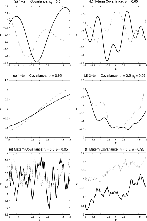
Figure 1: Response curves drawn from a GP. Each plot shows two (solid and dashed) random realizations. Plots (a)–(c) were obtained with the exponential covariance (7) and plot (d) with the 2-term formulation (3.1). Plots (e) and (f) show realizations from the matern construction. All curves employ a one-dimensional covariate.

We also consider a two-term covariance obtained by adding a second exponential term to (7), that is,

$$\hskip 16.0pt\mathbf{C} = \operatorname{Cov}(\mathbf{z}(\mathbf{X}))$$

$$= \frac{1}{\lambda_{a}}\mathbf{J}_{n}+\frac{1}{\lambda_{1,z}}\exp(-\mathbf{G}_{1})+\frac{1}{\lambda_{2,z}}\exp(-\mathbf{G}_{2}),\vspace*{4pt}$$

where $\mathbf{G}_{1}$ and $\mathbf{G}_{2}$ are parameterized as $\mathbf{P}_{1}\break=\operatorname{diag}(-\log(\rho_{1,1},\ldots,\rho_{1,p}))$ and $\mathbf{P}_{2}=\operatorname{diag}(-\log(\rho_{2,1},\break\ldots,\rho_{2,p}))$, respectively. As noted in Neal (2000), adding multiple terms results in rougher, more complex, surfaces while retaining the relative computational efficiency of the exponential formulation. For example, plot (d) of Figure 1 shows examples of surfaces that can be generated by employing the $2$-term covariance formulation with $(\rho_{1},\rho_{2})=(0.5,0.05)$ and $(\lambda_{1,z}=1,\lambda_{2,z}=8)$.

3.2 The Matern Construction

An alternative choice to the exponential covariance term is the Matern formulation. This introduces an explicit smoothing parameter, $\nu$, such that the resulting Gaussian process is $k$ times differentiable for $k\leq\nu$,

$$\hskip 7.0pt\mathbf{C}(z(\mathbf{x}_{i}),z(\mathbf{x}_{j}))$$

(9)

$$\hskip 7.0pt\quad=\frac{1}{2^{\nu-1}\Gamma(\nu)}\bigl{[}2\sqrt{\nu d(\mathbf{x}_{i},\mathbf{x}_{j})}\bigr{]}^{\nu}K_{\nu}\bigl{[}2\sqrt{\nu d(\mathbf{x}_{i},\mathbf{x}_{j})}\bigr{]},$$

with $d(\mathbf{x}_{i},\mathbf{x}_{j})=(\mathbf{x}_{i}-\mathbf{x}_{j})^{\prime}\mathbf{P}(\mathbf{x}_{i}-\mathbf{x}_{j})$, $K_{\nu}(\cdot)$ the Bessel function and $\mathbf{P}$ parameterized as in (7). Banerjee et al. (2008) employ such a construction with $\nu$ fixed to $0.5$ for modeling a spacial random effects process characterized by roughness. One recovers the exponential covariance term from the Matern construction in the limit as $\nu\rightarrow\infty$. However, Rasmussen and Williams (2006) point out that two formulations are essentially the same for $\nu>\frac{7}{2}$, as confirmed by our own simulations.

4 Prior Model for Bayesian Variable Selection

The unified modeling approach we have described allows us to put forward a general framework for variable selection that employs Bayesian methods and mixture priors for the selection of the predictors. In particular, variable selection can be achieved within the GP modeling framework by imposing “spike-and-slab” mixture priors on the covariance parameters in (7), that is,

$$\hskip 12.0pt\pi(\rho_{k}|\gamma_{k})=\gamma_{k}\mathbb{I}[0\leq\rho_{k}\leq 1]+(1-\gamma_{k})\delta_{1}(\rho_{k}),$$ (10)

for $k=1,\ldots,p$, with $\delta_{1}(\cdot)$ a point mass distribution at one. Clearly, $\rho_{k}=1$ causes the predictor $x_{k}$ to have no effect on the computation for the GP covariance matrix. This formulation is similar in spirit to the use of selection priors for linear regression models and is employed by Linkletter et al. (2006) in the univariate GP regression framework (3). Further Bernoulli priors are imposed on the selection parameters, that is, $\gamma_{k}\sim\operatorname{Bernoulli}(\alpha_{k})$ and Gamma priors are specified on the precision terms $(\lambda_{a},\lambda_{z})$.

Variable selection with a covariance matrix that employs two exponential terms as in (3.1) is more complex. In particular, one can select covariates separately for each exponential term by assigning a specific set of variable selection parameters to each term, that is, $(\bolds{\gamma}_{1},\bolds{\gamma}_{2})$ associated to $(\bolds{\rho}_{1},\bolds{\rho}_{2})$, and simply extending the single term formulation via independent spike-and-slab priors of the form

$$\hskip 10.0pt\pi(\rho_{1,k}|\gamma_{1,k})$$

(11)

$$\hskip 10.0pt\quad=\gamma_{1,k}\mathbb{I}[0\leq\rho_{1,k}\leq 1]+(1-\gamma_{1,k})\delta_{1}(\rho_{1,k}),$$

$$\hskip 10.0pt\pi(\rho_{2,k}|\gamma_{2,k})$$

(12)

$$\hskip 10.0pt\quad=\gamma_{2,k}\mathbb{I}[0\leq\rho_{2,k}\leq 1]+(1-\gamma_{2,k})\delta_{1}(\rho_{2,k}),$$

with $k=1,\ldots,p$. Assuming a priori independence of the two model spaces, Bernoulli priors can be imposed on the selection parameters, that is, $\gamma_{i,k}\sim\operatorname{Bernoulli}(\alpha_{i,k}),i=1,2$. This variable selection framework identifies the association of each covariate, $x_{k}$, to one or both terms. Final selection can then be accomplished by choosing the covariates in the union of those selected by either of the two terms. An alternative strategy for variable selection may employ a common set of variable selection parameters, $\bolds{\gamma}=(\gamma_{1},\ldots,\gamma_{p})$ for both $\bolds{\rho}_{1}$ and $\bolds{\rho}_{2}$, in a joint spike-and-slab (product) prior formulation,

$$\pi(\rho_{1,k},\rho_{2,k}|\gamma_{k})$$

$$\quad=\gamma_{k}\mathbb{I}[0\leq\rho_{1,k}\leq 1]\mathbb{I}[0\leq\rho_{2,k}\leq 1]$$ (13)

$$\qquad{}+(1-\gamma_{k})\delta_{1}(\rho_{1,k})\delta_{1}(\rho_{2,k}),$$

where we assume a priori independence of the parameter spaces, $\bolds{\rho}_{1}$ and $\bolds{\rho}_{2}$. This prior choice focuses more on overall covariate selection, rather than simultaneous selection and assignment to each term in (3.1). While we lose the ability to align the $\rho_{i,k}$ to each covariance function term, we expect to improve computational efficiency by jointly sampling $(\bolds{\gamma},\bolds{\rho}_{1},\bolds{\rho}_{2})$ at each iteration of the MCMC scheme as compared to a separate joint sampling on $(\bolds{\gamma}_{1},\bolds{\rho}_{1})$ and $(\bolds{\gamma}_{2},\bolds{\rho}_{2})$. Some investigation is done in Savitsky (2010).

5 Posterior Inference

The methods for posterior inference we are going to describe apply to all GP formulations, even though we focus our simulation work on the continuous and count data models. We therefore express the posterior formulation employing a generalized notation. First, we collect all parameters of the GP covariance matrix in $\bolds\Theta$ and write $\mathbf{C}=\mathbf{C}(\bolds{\Theta})$. For example, for covariance matrix of type (7) we have $\bolds{\Theta}=(\bolds{\rho},\lambda_{a},\lambda_{z})$. Next, we extend our notation to include the selection parameter $\bolds{\gamma}$ by using $\bolds{\Theta}_{\bolds{\gamma}}=(\bolds{\rho}_{\bolds{\gamma}},\lambda_{a},\lambda_{z})$ to indicate that $\rho_{k}=1$ when $\gamma_{k}=0$, for $k=1,\ldots,p$. For covariance of type (3.1) we write $\bolds{\Theta}_{\bolds{\gamma}}=\{\bolds{\Theta}_{\bolds{\gamma}_{1}},\bolds{\Theta}_{\bolds{\gamma}_{2}},\lambda_{a}\}$, where $\bolds{\gamma}=(\bolds{\gamma}_{1},\bolds{\gamma}_{2})^{\prime}$ and $\bolds{\Theta}_{\bolds{\gamma}_{i}}=(\bolds{\rho}_{i\bolds{\gamma}_{i}},\lambda_{i,z}),i\in\{1,2\}$ for prior of type (4)–(4) and $\bolds{\Theta}_{\bolds{\gamma}}=(\bolds{\rho}_{1\bolds{\gamma}},\bolds{\rho}_{2\bolds{\gamma}},\lambda_{a},\lambda_{1,z},\lambda_{2,z})$ for prior of type (4), and similarly for the Matern construction. Next, we define $D_{i}\in\{y_{i},\{s_{i},z(\mathbf{x}_{i})\}\}$ and $\mathbf{D}:=\{D_{1},\ldots,D_{n}\}$ to capture the observed data augmented by the unobserved GP variate, $\mathbf{z}(\mathbf{X})$, for the latent response models [such as model (2.1) for count data]. Finally, we set $\mathbf{h}:=\{r,\tau\}$ to group unique parameters $\notin\bolds{\Theta}_{\bolds{\gamma}}$ and we collect hyperparameters in $\mathbf{m}:=\{\mathbf{a},\mathbf{b}\}$, with $\mathbf{a}=\{a_{\lambda_{a}},a_{\lambda_{z}},a_{r},a_{\tau}\}$ and similarly for $\mathbf{b}$, where $\mathbf{a}$ and $\mathbf{b}$ include the shape and rate hyperparameters of the Gamma priors on the associated parameters. With this notation we can finally outline a generalized expression for the full conditional of $(\bolds{\gamma},\bolds{\rho}_{\bolds{\gamma}})$ as

$$\pi(\bolds{\gamma},\bolds{\rho}_{\bolds{\gamma}}|\bolds{\Theta}_{\bolds{\gamma}}\backslash\bolds{\rho}_{\bolds{\gamma}},\mathbf{D},\mathbf{h},\mathbf{m})$$

(14)

$$\quad\propto L^{a}(\bolds{\gamma},\bolds{\rho}_{\bolds{\gamma}}|\bolds{\Theta}_{\bolds{\gamma}}\backslash\bolds{\rho}_{\bolds{\gamma}},\mathbf{D},\mathbf{h},\mathbf{m})\pi(\bolds{\gamma}),$$

with $L^{a}$ the augmented likelihood. Notice that the term $\pi(\bolds{\rho}_{\bolds{\gamma}}|\bolds{\gamma})$ does not appear in (5) since $\pi(\rho_{k}|\break\gamma_{k})=1$, for $k=1,\ldots,p$.

5.1 Markov Chain Monte Carlo—Scheme 1

We first describe a Metropolis–Hastings scheme within Gibbs sampling to jointly sample $(\bolds{\gamma},\bolds{\rho}_{\bolds{\gamma}})$, which is an adaptation of the MCMC model comparison ($\mathrm{MC}^{3}$) algorithm originally outlined in Madigan and York (1995) and extensively used in the variable selection literature. As we are unable to marginalize over the parameter space, we need to modify the algorithm in a hierarchical fashion, using the move types outlined below. Additionally, we need to sample all the other nuisance parameters.

A generic iteration of this MCMC procedure comprises the following steps: [(2)]

Update $({\gamma},{\rho}_{{\gamma}})$: Randomly choose among three between-models transition moves: [(iii)]

Add: set $\gamma_{k}^{\prime}=1$ and sample $\rho_{k}^{\prime}$ from a $\mathcal{U}(0,1)$ proposal. Position $k$ is randomly chosen from the set of $k$’s where $\gamma_{k}=0$ at the previous iteration.

Delete: set $(\gamma_{k}^{\prime}=0,\rho_{k}^{\prime}=1)$. This results in covariate $x_{k}$ being excluded in the current iteration. Position $k$ is randomly chosen from among those included in the model at the previous iteration.

Swap: perform both an Add and Delete move. This move type helps to more quickly traverse a large covariate space. The proposed value $(\bolds{\gamma}^{\prime},\bolds{\rho}_{\bolds{\gamma}^{\prime}}^{\prime})$ is accepted with probability,

$$\alpha=\min\biggl{\{}1,\frac{\pi(\bolds{\gamma}^{\prime},\bolds{\rho}_{\bolds{\gamma}^{\prime}}^{\prime}|\bolds{\Theta}_{\bolds{\gamma}^{\prime}}\backslash\bolds{\rho}^{\prime}_{\bolds{\gamma}^{\prime}},\mathbf{D},\mathbf{h},\mathbf{m})q(\bolds{\gamma}|\bolds{\gamma}^{\prime})}{\pi(\bolds{\gamma},\bolds{\rho}_{\bolds{\gamma}}|\bolds{\Theta}_{\bolds{\gamma}}\backslash\bolds{\rho}_{\bolds{\gamma}},\mathbf{D},\mathbf{h},\mathbf{m})q(\bolds{\gamma}^{\prime}|\bolds{\gamma})}\biggr{\}},$$

where the ratio of the proposals $q(\bolds{\rho}_{\bolds{\gamma}})/q(\bolds{\rho}_{\bolds{\gamma}^{\prime}}^{\prime})$ drops out of the computation since we employ a $\mathcal{U}(0,1)$ proposal.

Execute a Gibbs-type move, Keep, by sampling from a $\mathcal{U}(0,1)$ all $\rho^{\prime}_{k}$’s such that $\gamma_{k}^{\prime}=1$. This move is not required for ergodicity, but it allows to perform a refinement of the parameter space within the existing model, for faster convergence.

Update $\{\lambda_{a},\lambda_{z}\}$: These are updated using Metropolis–Hastings moves with Gamma proposals centered on the previously sampled values.

Update $\mathbf{h}$: Individual model parameters in $\mathbf{h}$ are updated using Metropolis–Hastings moves with proposals centered on the previously sampled values.

Update $\mathbf{z}$: Jointly sample $\mathbf{z}$ for latent response models using the approach enumerated in Neal (1999) with proposal $\mathbf{z}^{\prime}=(1-\varepsilon^{2})^{1/2}\mathbf{z}+\varepsilon\mathbf{L}\mathbf{u}$, where $\mathbf{u}$ is a vector of i.i.d. standard Gaussian values and $\mathbf{L}$ is the Cholesky decomposition of the GP covariance matrix. For faster convergence $R$ consecutive updates are performed at each iteration.

Green (1995) introduced a Markov chain Monte Carlo method for Bayesian model determination for the situation where the dimensionality of the parameter vector varies iteration by iteration. Recently, Gottardo and Raftery (2008) have shown that the reversible jump can be formulated in terms of a mixture of singular distributions. Following the results given in their examples, it is possible to show that the acceptance probability of the reversible jump formulation is the same as in the Metropolis–Hastings algorithm described above, and therefore that the two algorithms are equivalent; see Savitsky (2010).

For inference, estimates of the marginal posterior probabilities of $\gamma_{k}=1$, for $k=1\ldots,p$, can be computed based on the MCMC output. A simple strategy is to compute Monte Carlo estimates by counting the number of appearances of each covariate across the visited models. Alternatively, Rao–Blackwellized estimates can be calculated by averaging the full conditional probabilities of $\gamma_{k}=1$. Although computationally more expensive, the latter strategy may result in estimates with better precision, as noted by Guan and Stephens (2011). In all simulations and examples reported below we obtained satisfactory results by estimating the marginal posterior probabilities by counts restricted to between-models moves, to avoid over-estimation.

5.2 Markov Chain Monte Carlo—Scheme 2

Next we enumerate a Markov chain Monte Carlo algorithm to directly sample $(\bolds{\gamma},\bolds{\rho}_{\bolds{\gamma}})$ with a Gibbs scan that employs a Metropolis acceptance step. We formulate a proposal distribution of a similar mixture form as the joint posterior by extending a result from Gottardo and Raftery (2008) to produce a move to $(\gamma_{k}=0,\rho_{k}=1)$, as well as to $(\gamma_{k}=1,\rho_{k}=[0,1))$.

A generic iteration of this MCMC procedure comprises the following steps: [(2)]

For $k=1,\ldots,p$ perform a joint update for ($\gamma_{k},\rho_{k})$ with two moves, conducted in succession: [(ii)]

Between-models: Jointly propose a new model such that if $\gamma_{k}=1$, propose $\gamma_{k}^{\prime}=0$ and set $\rho_{k}^{\prime}=1$; otherwise, propose $\gamma_{k}^{\prime}=1$ and draw $\rho_{k}^{\prime}\sim\mathcal{U}(0,1)$. Accept the proposal for $(\gamma_{k}^{\prime},\rho_{k}^{\prime})$ with probability,

$$\alpha=\min\biggl{\{}1,\frac{\pi(\gamma_{k}^{\prime},\rho_{k}^{\prime}|\bolds{\gamma}_{(k)}^{\prime},\bolds{\Theta}_{\bolds{\gamma}_{(k)}^{\prime}},\mathbf{D},\mathbf{h},\mathbf{m})}{\pi(\gamma_{k},\rho_{k}|\bolds{\gamma}_{(k)}^{\prime},\bolds{\Theta}_{\bolds{\gamma}_{(k)}^{\prime}},\mathbf{D},\mathbf{h},\mathbf{m})}\biggr{\}},$$

where now $\bolds{\gamma}_{(k)}^{\prime}:=(\gamma_{1}^{\prime},\ldots,\gamma_{k-1}^{\prime},\gamma_{k+1},\ldots,\gamma_{p})$ and similarly for $\bolds{\rho}_{(k)}^{\prime}\in\bolds{\Theta}_{\bolds{\gamma}_{(k)}^{\prime}}$. The joint proposal ratio for $(\gamma_{k},\rho_{k})$, reduces to $1$ since we employ a $\mathcal{U}(0,1)$ proposal for $\rho_{k}\in[0,1]$ and a symmetric Dirac measure proposal for $\gamma_{k}$.

Within model: This move is performed only if we sample $\gamma_{k}^{\prime}=1$ from the between-models move, in which case we propose $\gamma_{k}^{\prime\prime}=1$ and, as before, draw $\rho_{k}^{\prime\prime}\sim\mathcal{U}(0,1)$. Similar to the between-models move, accept the joint proposal for $(\gamma_{k}^{\prime\prime},\rho_{k}^{\prime\prime})$ with probability,

$$\alpha=\min\biggl{\{}1,\frac{\pi(\gamma_{k}^{\prime\prime},\rho_{k}^{\prime\prime}|\bolds{\gamma}_{(k)}^{\prime},\bolds{\Theta}_{\bolds{\gamma}_{(k)}^{\prime}},\mathbf{D},\mathbf{h},\mathbf{m})}{\pi(\gamma_{k}^{\prime},\rho_{k}^{\prime}|\bolds{\gamma}_{(k)}^{\prime},\bolds{\Theta}_{\bolds{\gamma}_{(k)}^{\prime}},\mathbf{D},\mathbf{h},\mathbf{m})}\biggr{\}},$$

which further reduces to just the ratio of posteriors since we propose a move within the current model and utilize a $\mathcal{U}(0,1)$ proposal for $\rho_{k}$.

Sample the parameters $\{\lambda_{a},\lambda_{z},\mathbf{h}\}$ and latent responses $\mathbf{z}$ as outlined in scheme 1.

In simulations we also investigate performances of an adaptive scheme that employs a proposal with tuning parameters adapted based on “learning” from the data. In particular, we employ the method of Haario, Saksman and Tamminen (2001) for our Bernoulli proposal for $\gamma|\alpha$ to successively update the mean parameter, $\alpha_{k},k=1,\ldots,p$, based on prior sampled values for $\gamma_{k}$. The construction does not require additional likelihood computations and it is expected to achieve more rapid convergence in the model space than the nonadaptive scheme. Roberts and Rosenthal (2007) and Ji and Schmidler (2009) note conditions under which adaptive schemes achieve convergence to the target posterior distribution.

Schemes 1 and 2 we enumerated above may be easily modified when employing the $2$-term covariance formulation (3.1); see Savitsky (2010).

5.3 Prediction

Let ${\mathbf{z}_{f}}=\mathbf{z}(\mathbf{X}_{f})$ be an $n_{f}\times 1$ latent vector of future cases. We use the regression model (3) to demonstrate prediction under the GP framework. The joint distribution over training and test sets is defined to be $\mathbf{z}_{*}:=[\mathbf{z}^{\prime},\mathbf{z}_{f}^{\prime}]^{\prime}\sim\mathcal{N}(\mathbf{0},\mathbf{C}_{n+n_{f}})$ with covariance,

$$\mathbf{C}_{n+n_{f}}:=\pmatrix{\mathbf{C}_{(\mathbf{X},\mathbf{X})}&\mathbf{C}_{(\mathbf{X},\mathbf{X}_{f})}\cr\mathbf{C}_{(\mathbf{X}_{f},\mathbf{X})}&\mathbf{C}_{(\mathbf{X}_{f},\mathbf{X}_{f})}},$$

where $\mathbf{C}_{(\mathbf{X},\mathbf{X})}:=\mathbf{C}_{(\mathbf{X},\mathbf{X})}(\bolds{\Theta})$. The conditional joint predictive distribution over the test cases, $\mathbf{z}_{f}|\mathbf{z}$, is also multivariate normal distribution with expectation $\mathbb{E}[\mathbf{z}_{f}|\mathbf{z}]=\mathbf{C}_{(\mathbf{X}_{f},\mathbf{X})}\mathbf{C}_{(\mathbf{X},\mathbf{X})}^{-1}\mathbf{z}$. Estimation is based on the posterior MCMC samples. Here we take a computationally simple approach by first estimating $\hat{\mathbf{z}}$ as the mean of all sampled values of $\mathbf{z}$, defining

$$\mathbf{D}(\bolds{\Theta}):=\mathbf{C}_{(\mathbf{X}_{f},\mathbf{X})}\mathbf{C}_{(\mathbf{X},\mathbf{X})}^{-1}\hat{\mathbf{z}},$$ (15)

and then estimating the response value as

$$\hat{\mathbf{y}}_{f}=\hat{\mathbf{z}}_{f}|\hat{\mathbf{z}}=\frac{1}{K}\sum_{t=1}^{K}\mathbf{D}(\bolds{\Theta}^{(t)}),$$ (16)

with $K$ the number of MCMC iterations and where calculations of the covariance matrices in (15) are restricted to the variables selected based on the marginal posterior probabilities of $\gamma_{k}=1$. A more coherent estimation procedure, that may return more precise estimates but that is also computationally more expensive, would compute Rao–Blackwellized estimates by averaging the predictive probabilities over all visited models; see Guan and Stephens (2011). In the simulations and examples reported below we have calculated (16) using every 10th MCMC sampled value, to provide a relatively less correlated sample and save on computational time. In addition, when computing the variance product term in (15), we have employed the Cholesky decomposition $\mathbf{C}=\mathbf{L}\mathbf{L}^{\prime}$, following Neal (1999), to avoid direct computation of the inverse of $\mathbf{C}_{(\mathbf{X},\mathbf{X})}$.

For categorical data models, we may predict the new class labels, $\mathbf{t}_{f}$, via the rule of largest probability in the case of a binary logit model, with estimated latent realizations $\hat{\mathbf{z}}_{f}$, and via data augmentation based on the values of $\hat{\mathbf{y}}_{f}$ in the case of a binary probit model.

5.3.1 Survival Function Estimation

For survival data it is of interest to estimate the survivor function for a new subject with unknown event time, $T_{i}$, and associated $z_{f,i}:=z_{f,i}(\mathbf{x}_{f,i})$. This is defined as

$$P(T_{i}\geq t|z_{f,i},\mathbf{z}) = S_{i}(t|z_{f,i},\mathbf{z})$$

$$= S_{0}(t|\mathbf{z})^{\exp(z_{f,i})}.$$

When using the partial likelihood formulation an empirical Bayes estimate of the baseline survivor function, $S_{0}(t|\mathbf{z})$, must be calculated, since the model does not specifically enumerate the baseline hazard. Weng and Wong (2007), for example, propose a method that discretizes the likelihood to produce an estimator with the useful property that it cannot take negative values. Accuracy of this estimate may be potentially improved by Rao–Blackwellizing the computation by averaging over the MCMC runs.

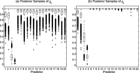
Figure 2: Use of variable selection parameters: Simulated data $(n=80,p=20)$. Box plots of posterior samples for $\rho_{k}\in[0,1]$. Plots (a) and (b) demonstrate selection without and with, respectively, the inclusion of the selection parameter $\bolds{\gamma}$.

6 Simulation Study

6.1 Parameter Settings

In all simulations and applications reported in this paper we set both priors on $\lambda_{a}$ and $\lambda_{z}$ as $\mathcal{G}(1,1)$. We did not observe any strong sensitivity to this choice. In particular, we considered different choices of the two parameters of these Gammma priors in the range $(0.01,1)$, keeping the prior mean at 1 but with progressively larger variances, and observed very little change in the range of posterior sampled values. We also experimented with prior mean values of $10$ and $100$, which produced only a small impact on the posterior. For model (3) we set $r\sim\mathcal{G}(a_{r},b_{r})$ with $(a_{r},b_{r})=(2,0.1)$ to reflect our a priori expected residual variance. For the count model (2.1), we set $\tau\sim\mathcal{G}(1,1)$. For survival data, when using the full likelihood from Kalbfleisch (1978) we specified a $\mathcal{G}(1,1)$ prior for both the parameter of the exponential base distribution and the concentration parameter of the Gamma process prior on the baseline.

Some sensitivity on the Bernoulli priors on the $\gamma_{k}$’s is, of course, to be expected, since these priors drive the sparsity of the model. Generally speaking, parsimonious models can be selected by specifying $\gamma_{k}\sim\operatorname{Bernoulli}(\alpha_{k})$ with $\alpha_{k}=\alpha$ and $\alpha$ a small percentage of the total number of variables. In our simulations we set $\alpha_{k}$ to $0.025$. We observed little sensitivity in the results for small changes around this value, in the range of 0.01–0.05, though we would expect to see significant sensitivity for much higher values of $\alpha$. We also investigated sensitivity to a Beta hyperprior on $\alpha$; see below.

When running the MCMC algorithms independent chain samplers with $\mathcal{U}(0,1)$ proposals for the $\rho_{k}$’s have worked well in all applications reported in this paper, where we have always approximately achieved the target acceptance rate of 40–60% indicating efficient posterior sampling.

6.2 Use of Variable Selection Parameters

We first demonstrate the advantage of introducing selection parameters in the model. Figure 2 shows results with and without the inclusion of the variable selection parameter vector $\bolds{\gamma}$ on a simulated scenario with a kernel that incorporates both linear and nonlinear associations. The observed continuous response, $y$, is constructed from a mix of linear and nonliner relationships to $4$ variables, each generated from a $\mathcal{U}(0,1)$,

$$y=x_{1}+x_{2}+\sin(3x_{3})+\sin(5x_{4})+\varepsilon,$$

with $\varepsilon\sim\mathcal{N}(0,\sigma^{2})$ and $\sigma=0.05$. Additional variables are randomly generated, again from $\mathcal{U}(0,1)$. In this simulation we used $(n,p)=(80,20)$. We ran 70,000 MCMC iterations, of which 10,000 were discarded as burn-in.

Plot (a) of Figure 2 displays box plots of the MCMC samples for the $\rho_{k}^{\prime}s,k=1,\ldots,20$, for the case of no variable selection, that is, by using a simple “slab” prior on the $\rho_{k}$’s. As both Linkletter et al. (2006) and Neal (2000) note, the single covariates demonstrate an association to the response whose strength may be assessed utilizing the distance of the posterior samples of the $\rho_{k}$’s from $1$. One notes that, according to this criterion, the true covariates are all selected. It is conceivable, however, for some of the unrelated covariates to be selected using the same criterion, since the $\rho_{k}$’s all sample below $1$, and that this problem would be compounded as $p$ grows. Plot (b) of Figure 2, instead, captures results from employing the variable selection parameters $\bolds{\gamma}$ and shows how the inclusion of these parameters results in the sampled values of the $\rho_{k}$’s for variables unrelated to the response being all pushed up against $1$.

This simple simulated scenario also helps us to illustrate a couple of other features. First, a single exponential term in (7) is able to capture a wide variety of continuous response surfaces, allowing a great flexibility in the shape of the response surface, with the linear fit being a subset of one of many types of surfaces that can be generated. Second, the effect of covariates with higher-order polynomial-like association to the response is captured by having estimates of the corresponding $\rho_{k}$’s further away from 1; see, for example, covariate $x_{4}$ in Figure 2 which expresses the highest order association to the response.

Table 1: Large $p$: Simulations for continuous, count and survival data models with $(n,p)=(100,1{,}000)$

	Continuous data	Count data	Cox model
Coefficients:
$a_{1}$	$1.0$	$1.6$	$-$$3.0$
$a_{2}$	$1.0$	$1.6$	$-2.5$
$a_{3}$	$1.0$	$1.6$	$-$$3.5$
$a_{4}$	$1.0$	$1.6$	$-3.0$
$a_{5}$	$1.0$	$1.0$	$-$$1.0$
$a_{6}$	$3.0$	$3.0$	$-$$3.0$
$a_{7}$	$1.0$	$1.0$	$-1.0$
$a_{8}$	$5.0$	$5.0$	$-$$5.0$
Model	Identity link	$\log(\lambda)=y$	$S(t|y)=\exp[-H_{0}(t)\exp(y)]$
		$t\sim\operatorname{Pois}(\lambda)$	$H_{0}(t)=\lambda t,\lambda=0.2$
			$t=M/(\lambda\exp(y)),M\sim\operatorname{Exp}(1)$
			$5\%$ uniform randomly censored,
			$t_{\mathrm{cens}}=\mathcal{U}(0,t_{\mathrm{event}})$
Train/test	$100/20$	$100/20$	$100/60$
Correctly selected	$6$ out of $6$	$6$ out of $6$	$5$ out of $6$
False positives	$0$	$0$	$0$
MSPE (normalized)	$0.0067$	$0.045$	see Figure 4

6.3 Large $p$

Next we show simulation results on continuous, count and survival data models, for $(n,p)=(100,\break 1{,}000)$. We employ an additive term as the kernel for all models,

$$y = a_{1}x_{1}+a_{2}x_{2}+a_{3}x_{3}+a_{4}x_{4}$$

$${}+a_{5}\sin(a_{6}x_{5})+a_{7}\sin(a_{8}x_{6})+\varepsilon.$$

The functional form for the simulation kernel is designed so that the first four covariates express a linear relationship to the response while the next two express nonlinear associations. Model-specific coefficient values are displayed in Table 1. Methods employed to randomly generate the observed count and event time data from the latent response kernel are also outlined in the table. For example, the kernel captures the $\log$-mean of the Poisson distribution used to generate count data, and it is used to generate the survivor function that is inverted to provide event time data for the Cox model. As in the previous simulation, all covariates are generated from $\mathcal{U}(0,1)$.

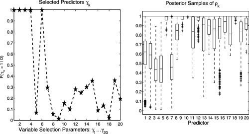
Figure 3: Cox GP model with large $p$: Simulated data $(n=100,p=1{,}000)$. Posterior distributions for $\gamma_{k}=1$ and box plots of posterior samples for $\rho_{k}$.

We set the hyperparameters as described in Section 6.1. We used MCMC scheme 1 and increased the number of total iterations, with respect to the simpler simulation with only $p=20$, to 800,000 iterations, discarding half of them for burn-in.

Results are reported in Table 1. While the continuous and count data GP models readily assigned high marginal posterior probabilities to the correct covariates (figures not shown), the Cox GP model correctly identified only $5$ of $6$ predictors; see Figure 3 for the posterior distributions of $\gamma_{k}=1$ and the box plots for the posterior samples of $\rho_{k}$ for this model (for readability, only the first $20$ covariates are displayed). The predictive power for the continuous and count data models was assessed by normalizing the mean squared prediction error (MSPE) with the variance of the test set. Excellent results were achieved in our simulations. For the Cox GP model, the averaged survivor function estimated on the test set is shown in Figure 4, where we observe a tight fit between the estimated curve and the Kaplan–Meier empirical estimate constructed from the same test data.

Though for the Cox model we only report results obtained using the partial likelihood formulation, we conducted the same simulation study with the model based on the full likelihood of Kalbfleisch (1978). The partial likelihood model formulation produced more consistent results across multiple chains, with the same data, and was able to detect much weaker signals. The Kalbfleisch (1978) model did, however, produce lower posterior values near $0$ for nonselected covariates, unlike the partial likelihood formulation, which shows values typically from 10–40%, pointing to a potential bias toward false positives.

Additional simulations, including larger sample sizes cases, are reported in Savitsky (2010).

Table 2: Efficiency comparison of GP MCMC methods

	MCMC scheme 2		MCMC scheme 1
	Adaptive	Nonadaptive
Iterations (computation)	$5{,}000$	$5{,}000$	$500{,}000$
Autocorrelation time
$\rho_{6}$	$310$	$82$	$441$
$\rho_{8}$	$59$	$35$	$121$
Computation
CPU-time (sec)	$980$	$4{,}956$	$10{,}224$

6.4 Comparison of MCMC Methods

We compare the 2 MCMC schemes previously described for posterior inference on $(\bolds{\gamma},\bolds{\rho})$ on the basis of sampling and computational efficiency. We use the univariate regression simulation kernel

$$y = x_{1}+0.8x_{2}+1.3x_{3}+\sin(x_{4})+\sin(3x_{5})$$

$${}+\sin(5x_{6})+(1.5x_{7})(1.5x_{8})+\varepsilon,$$

with $\varepsilon\sim\mathcal{N}(0,\sigma^{2})$ and $\sigma=0.05$. We utilize $1{,}000$ covariates with all but the first $8$ defined as nuisance. We use a training and a validation set of $100$ observations each.

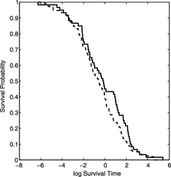
Figure 4: Cox GP model with large $p$: Simulated data $(n=100,p=1{,}000)$. Average survivor function curve on the validation set (dashed line) compared to the Kaplan–Meier empirical estimate (solid line).

The two schemes differ in the way they update $(\bolds{\gamma},\bolds{\rho})$. While scheme 1 samples either one or two positions in the model space on each iteration, scheme 2 samples $(\gamma_{k},\rho_{k})$ for each of the $p$ covariates. Because of this a good “rule-of-thumb” should employ a number of iterations for scheme 1 which is roughly $p$ times the number of iterations employed for scheme 2. The use of the Keep move in scheme 1, however, reduces the need of scaling the number of iterations by exactly $p$, since all $\rho_{k}$’s are sampled at each iteration. In our simulations we found stable convergence under moderate correlation among covariates for scheme 2 in $5{,}000$ iterations and for scheme 1 in $500{,}000$ iterations. For both schemes, we discarded half of the iterations as burn-in. The CPU run times we report in Table 2 are based on utilization of Matlab with a 2.4 GHz Quad Core (Q6600) PC with 4 GB of RAM running 64-bit Windows XP.

We compared sampling efficiency looking at autocorrelation for selected $\rho_{k}$. The autocorrelation time is defined as one plus twice the sum of the autocorrelations at all lags and serves as a measure of the relative dependence for MCMC samples. We used the number of MCMC iterations divided by this factor as an “effective sample size.” We followed a procedure outlined by Neal (2000) and ran first scheme 2 for $1{,}000$ iterations, to obtain a state near the posterior distribution. We then employed this state to initiate a chain for each of the two schemes. We ran scheme 2 for an additional $2{,}000$ iterations and scheme 1 for $200{,}000$ (using the last $2{,}000$ draws for each of the target $\rho_{k}$ for final comparison). For scheme 2 we used both the adaptive and nonadaptive versions. Table 2 reports results for $\rho_{8}$, aligned to a covariate expressing a linear interaction, and for $\rho_{6}$, for a highly nonlinear interaction. We observe that both versions of scheme 2 express notable improvements in computational efficiency as compared to scheme 1. We note, however, that the adaptive scheme method produces draws of higher autocorrelation than the nonadaptive method.

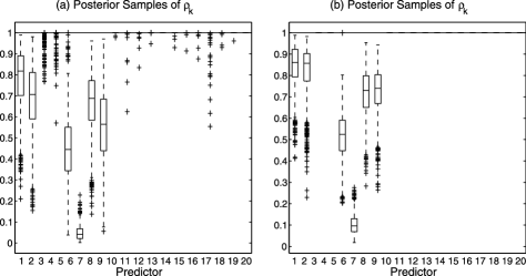
Figure 5: Prior Sensitivity for $\rho_{k}|\gamma_{k}=1\sim\operatorname{Beta}(a,b)$: Box plots of posterior samples for $\rho_{k}$ for $(a,b)=(0.5,0.5)$—plot (a)—and $(a,b)=(2.0,2.0)$—plot (b).

Table 3: Prior sensitivity for $\rho_{k}|\gamma_{k}=1\sim\operatorname{Beta}(a,b)$. Results are reported as (number of false negatives)${}/{}$(normalized MSPE)

$\bolds{b\backslash a}$	$\bolds{0.5}$	$\bolds{1.0}$	$\bolds{2.0}$
0.5	$2/0.18$	$2/0.15$	$2/0.18$
1.0	$1/0.14$	$1/0.16$	$2/0.18$
2.0	$1/0.15$	$2/0.16$	$2/0.17$

6.5 Sensitivity Analysis

We begin with a sensitivity analysis on the prior for $\rho_{k}|\gamma_{k}=1$. Table 3 shows results under a full factorial combination for hyperparameters $(a,b)$ of a Beta prior construction, where we recall $\operatorname{Beta}(1,1)\equiv\mathcal{U}(0,1)$. Results were obtained with the univariate regression simulation kernel

$$y = x_{1}+x_{2}+\sin(1.5x_{3})\sin(1.5x_{4})+\sin(3x_{5})$$

$${}+\sin(3x_{6})+(1.5x_{7})(1.5x_{8})+\varepsilon,$$

with $\varepsilon\sim\mathcal{N}(0,\sigma^{2})$ and where we employed a higher error variance of $\sigma=0.28$. As before, we employ $1{,}000$ covariates with all but the first $8$ defined as nuisance. A training sample of $110$ was simulated, along with a test set of $100$ observations. We employed the adaptive scheme 2, with $5{,}000$ iterations, half discarded as burn-in.

Figure 5 shows box plots of posterior samples for $\rho_{k}$ for two symmetric alternatives, $1\dvtx(a,b)=(0.5,0.5)$ (U-shaped) and $2\dvtx(a,b)=(2.0,2.0)$ (symmetric unimodal). For scenario 2 we observe a reduction in posterior jitter on nuisance covariates and a stabilization of posterior sampling for associated covariates, but also a greater tendency to exclude $x_{3},x_{4}$. One would expect the differences in posterior sampling behavior across prior hyperparameter values to decline as the sample size increases. Table 3 displays the number of nonselected true variables (false negatives), out of 8, along with the normalized MSPEs for all scenarios. There were no false positives to report across all hyperparameter settings. Overall, results are similar across the chosen settings for $(a,b)$, with slightly better performances for $a<1$ and $b\geq 1$, corresponding to strictly decreasing shapes that aid selection by pushing more mass away from 1, increasing the prior probability of the good variables to be selected, especially in the presence of a large number of noisy variables.

Next we imposed a Beta distribution on the hyperparameter $\alpha$ of the priors $\gamma_{k}\sim\operatorname{Bernoulli}(\alpha)$ for covariate inclusion. We follow Brown, Vannucci and Fearn (1998a) to specify a vague prior by setting the mean of the Beta prior to $0.025$, reflecting a prior expectation for model sparsity, and the sum of the two parameters of the distribution to $2$. We ran the same univariate regression simulation kernel as above with the hyperparameter settings for the Beta prior on $\rho_{k}$ equal to $(1,1)$ and obtained the same selection results as in the case of $\alpha$ fixed and a slightly lower normalized MSPE of $0.14$.

Table 4: Ozone data: Results

Prior on $\bolds{g}$	$\bolds{\mathcal{M}}_{\bolds{\gamma}}$	$\mathbf{p}_{\bolds{\gamma}}$	RMSPE
Local empirical Bayes	$X_{5},X_{6},X_{7},X_{6}^{2},X_{7}^{2},X_{3}X_{5}$	6	4.5
Hyper-$g$ ($a=4$)	$X_{5},X_{6},X_{7},X_{6}^{2},X_{7}^{2},X_{3}X_{5}$	6	4.5
Fixed (BIC)	$X_{5},X_{6},X_{7},X_{6}^{2},X_{7}^{2},X_{3}X_{5}$	$6$	4.5
Brown, Vannucci and Fearn (2002)	$X_{1}X_{6},X_{1}X_{7},X_{6}X_{7},X_{1}^{2},X_{3}^{2},X_{7}^{2}$	6	4.5
GP model	$X_{3},X_{6},X_{7}$	3	3.7

Last, we explored performances with respect to correlation among the predictors. We utilized the same kernel as above with $8$ true predictors from which to construct the response. We then induced a $70\%$ correlation among $20$ randomly chosen nuisance covariates and the true predictor $x_{6}$. We found $2$ false negatives and $1$ false positive, which demonstrates a relative selection robustness under correlation. We did observe a significant decline in normalized MSPE, however, to $0.33$, as compared to previous runs.

7 Benchmark Data Applications

We now present results on two data sets often used in the literature as benchmarks. For both analyses we performed inference by using the MCMC—scheme 2, with $5{,}000$ iterations and half discarded as burn-in.

7.1 Ozone data

We start by revisiting the ozone data, first analyzed for variable selection by Breiman and Friedman (1985) and more recently by Liang et al. (2008). This data set supplies integer counts for the maximum number of ozone particles per one million particles of air near Los Angeles for $n=330$ days and includes an associated set of $8$ meteorological predictors. We held out a randomly chosen set of $165$ observations for validation.

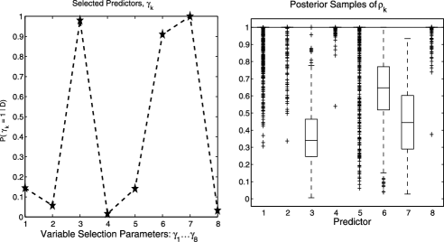
Figure 6: Ozone data: Posterior distributions for $\gamma_{k}=1$ and box plots of posterior samples for $\rho_{k}$.

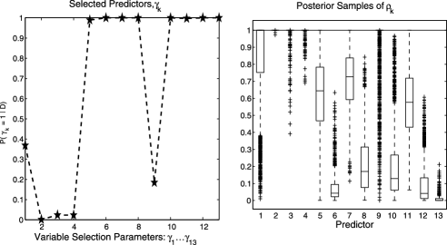
Figure 7: Boston housing data: Posterior distributions for $\gamma_{k}=1$ and box plots of posterior samples for $\rho_{k}$.

Liang et al. (2008) use a linear regression model including all linear and quadratic terms for a total of $p=44$ covariates. They achieve variable selection by imposing a mixture prior on the vector $\bolds{\beta}$ of regression coefficients and specifying a $g$-prior of the type $\bolds{\beta}_{\bolds{\gamma}}|\phi\sim\mathcal{N}(\mathbf{0},\frac{g}{\phi}(\mathbf{X}_{\bolds{\gamma}}^{T}\mathbf{X}_{\bolds{\gamma}})^{-1})$. Their results are reported in Table 4 with various formulations for $g$. In particular, the local empirical Bayes method offers a model-dependent maximizer of the marginal likelihood on $g$, while the hyper-$g$ formulation with $a=4$ is one member of a continuous set of hyper-prior distributions on the shrinkage factor, $g/(1+g)\sim\operatorname{Beta}(1,a/2-1)$. Since the design matrix expresses a high condition number, a situation that can at times induce poor results with $g$-priors, we additionally applied the method of Brown, Vannucci and Fearn (2002) who used a mixture prior of the type $\bolds{\beta}_{\bolds{\gamma}}\sim\mathcal{N}(\mathbf{0},c\mathbf{I})$. Results shown in Table 4 were obtained from the Matlab code made available by the authors.

Though previous variable selection work on the ozone data all choose a Gaussian likelihood, a more precise approach employs a discrete Poisson or negative binomial formulation on data with low count values, or a log-normal approximation where counts are high. With a maximum value of $38$ and a mean of $11$ we chose to model the data with the negative-binomial count data model (2.1). We used the same hyperparameter settings as in our simulation study. Results are shown in Figure 6. By selecting, for example, the best 3 variables, we achieve a notable decrease in the root-MSPE as compared to the linear models. Also, by allowing an a priori unspecified functional form for how covariates relate to the response, we end up selecting a much more parsimonious model, although, of course, we lose in interpretability of the selected terms, with respect to linear formulations that specifically include linear, quadratic and interactions terms in the model.

7.2 Boston Housing data

Next we utilize the Boston Housing data set, also analyzed by Breiman and Friedman (1985), who used an additive model and employed an algorithm to empirically determine the functional relationship for each predictor. This data set relates $p=13$ predictors to the median value of owner-occupied homes in each of $n=506$ census tracts in the Boston metropolitan area. As with the previous data set, we held out a random set of $250$ observations to assess prediction.

We employed the continuous data model (3) with the same hyperparameter settings as in our simulations. The four predictors chosen by Breiman and Friedman (1985), $(x_{6},x_{10},x_{11},x_{13}),$ had all marginal posterior probability of inclusion greater than 0.9 in our model. Other variables with high marginal posterior probability were $(x_{5},x_{7},x_{8},x_{12})$. The adaptability of the GP response surface is illustrated with closer examination of covariate $x_{5}$, which measures the level of nitrogen oxide (NOX), a pollutant emitted by cars and factories. At low levels, indicating proximity to jobs, $x_{5}$ presents a positive association to the response, and at high levels, indicating overly industrialized areas, a negative association. This inverted parabolic association over the covariate range probably drove its exclusion in the model of Breiman and Friedman (1985). The GP formulation is, however, able to capture this strong nonlinear relationship as is noted in Figure 7. By using only the subset of the best eight predictors, we achieved a normalized MSE of $0.1$ and a prediction $R^{2}$ of $0.9$, very close to the value of $0.89$ reported by Breiman and Friedman (1985) on the training data.

We also employed the Matern covariance construction (3.2), which we recall employs an explicit smoothing parameter, $\nu\in[0,\infty)$. While selection results were roughly similar, the prediction results for the Matern model were significantly worse than the exponential model, with a normalized MSPE of $0.16$, probably due to overfitting. It is worth noticing that the more complex form for the Bessel function increases the CPU computation time by a factor of 5–10 under the Matern covariance as compared to the exponential construction.

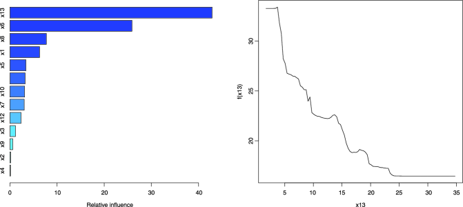
Figure 8: Boston housing data: GBM covariate analysis. Left-hand chart provides variables importance, normalized to sum up to 100. Right-hand plot enumerates partial association of $x_{13}$ to the response.

For comparison, we looked at GBMs. We used version 3.1 of the gbm package for the R software environment. We utilized the same training and validation data as above. After experimentation and use of $10$-fold cross-validation, we chose a small value for the input regularization parameter, $\nu=0.0005$, to provide a smoother fit that prevents overfitting. Larger values of $\nu$ resulted in higher prediction errors. The GBM was run for $50{,}000$ iterations to achieve minimum fit error. The result provided a normalized MSPE of $0.13$ on the test set, similar to, though slightly higher than, the GP result. The left-hand chart of Figure 8 displays the relative covariate importance. Higher values correspond to $(x_{13},x_{6},x_{8})$, and agree with our GP results. A number of other covariates show similar importance values to one another, though lower than these top $3$, making it unclear as to whether they are truly related or nuisance covariates. Similar conclusions are reported by other authors. For example, Tokdar, Zhu and Ghosh (2010) analyze a subset of the same data set with a Bayesian density regression model based on logistic Gaussian processes and subspace projections and found $(x_{13},x_{6})$ as the most influential predictors, with a number of others having a mild influence as well. The right-hand plot supplies a partial dependence plot obtained by the GBM for variable $x_{13}$ by averaging over the associations for the other covariates. We note that the nonlinear association is not constrained to be smooth under GBM.

8 Discussion

In this paper we have presented a unified modeling approach via Gaussian processes that extends to data from the exponential dispersion family and to survival data. Such model formulation allows for nonlinear associations of the predictors to the response. We have considered, in particular, continuous, categorical and count responses and survival data. Next we have addressed the important problem of selecting variables from a set of possible predictors and have put forward a general framework that employs Bayesian variable selection methods and mixture priors for the selection of the predictors. We have investigated strategies for posterior inference and have demonstrated performances on simulated and benchmark data. GP models provide a parsimonious approach to model formulation with a great degree of freedom for the data to define the fit. Our results, in particular, have shown that GP models can achieve good prediction performances without the requirement of prespecifying higher order and nonlinear additive functions of the predictors. The benchmark data applications have shown that a GP formulation may be appropriate in cases of heterogeneous covariates, where the inability to employ an obvious transformation would requirehigher order polynomial terms in an additive linear fashion, or even in the case of a homogeneous covariate space where the transformation overly reduces structure in the data. Our simulation results have further highlighted the ability of the GP formulation to manage data sets with $p\gg n$.

A challenge in the use of variable selection methods in the GP framework is to manage the numerical instability in the construction of the GP covariance matrix. In the Appendix we describe a projection method to reduce the effective dimension of this matrix. Another practical limitation of the models we have described is the difficulty to use them with qualitative predictors. Qian, Wu and Wu (2008) provide a modification of the GP covariance kernel that allows for nominal qualitative predictors consisting of any number of levels. In particular, the authors model the covariance structure under a mixture of qualitative and quantitative predictors by employing a multiplicative factor against the usual GP kernel for each qualitative predictor to capture the by-level categorical effects.

Some generalization of the methods we have presented are possible. For example, as with GLM models, we may employ an additional set of variance inflation parameters in a similar construction to Neal (1999) and others to allow for heavier tailed distributions while maintaining the conjugate framework.

Appendix: Computational Aspects

We focus on the exponential form (7) and introduce an efficient computational algorithm to generate ${\bf C}$. We also review a method of Banerjee et al. (2008) to approximate the inverse matrix that employs a random subset of observations and provide a pseudo-code.

.1 Generating the Covariance Matrix $\mathbf{C}$

Let us begin with the quadratic expression, $\mathbf{G}=\{g_{i,j}\}$ in (7). We rewrite $g_{i,j}=A_{i,j}^{\prime}[-\log(\bolds{\rho})]$ with $A_{i,j}$ constructed as a $p\times 1$ vector of term-by-term squared differences, $(x_{ik}-x_{jk})^{2},k=1,\ldots,p$. We may directly employ the $p\times 1$ vector, $\bolds{\rho}$, as $\mathbf{P}$ is diagonal. As a first step, we may then directly compute $\mathbf{G}=\mathbf{A}[-\log(\bolds{\rho})]$, where $\mathbf{A}$ is $n\times n\times p$. We are, however, able to reduce the more complex structure of $\mathbf{A}$ to a two dimensional matrix form by simply stacking each $\{i,j\}$ row of dimension $1\times p$ under each other such that our revised structure, $\mathbf{A}^{*}$, is of dimension $n^{2}\times p$ and the computation, $\mathbf{G}=\mathbf{A}^{*}[-\log(\bolds{\rho})]$, reduces to a series of inner products. Next, we note that $\log(\rho_{k})=0$ for $\rho_{k}=1$. So we may reduce the dimension for each of the $n^{2}$ inner products by reducing the dimension of $\bolds{\rho}$ to the $p_{\bolds{\gamma}}<p$ nontrivial covariates. We may further improve efficiency by recognizing that since our resultant covariance matrix, $\mathbf{C}$, is symmetric positive definite, we need only compute the inner products for a reduced set of unique terms (by removing redundant rows from $\mathbf{A}^{*}$) and then “re-inflate” the result to a vector of the correct length. Finally, we exponentiate this vector, multiply the nonlinear weight ($1/\lambda_{z}$), add the affine intercept term, ($1/\lambda_{a}$), and then reshape this vector into the resulting $n\times n$ matrix, $\mathbf{C}$. The resulting improvement in computational efficiency at $n=100$ from the naive approach that employs double loops of inner products is on the order of $500$ times.

Our MCMC scheme 2 proposes a change to $\rho_{k}\in\bolds{\rho}$, one-at-a-time, conditionally on $\bolds{\rho}_{-k}$ and the other sampled parameters. Changing a single $\rho_{k}$ requires updating only one column of the inner product computation of $\mathbf{A}^{*}$ and $[-\log(\bolds{\rho})]$. Rather than conducting an entire recomputation for $\mathbf{C}$, we multiply the $k$th column of $\mathbf{A}^{*}$ (with number of rows reduced to only unique terms in $\mathbf{C}$) by $\log(\frac{\rho_{k,\mathrm{prop}}}{\rho_{k,\mathrm{old}}})$, where “prop” means the proposed value for $\rho_{k}$. This result is next exponentiated (to a covariance kernel), re-inflated and shaped into an $n\times n$ matrix, $\bolds{\Delta}$. We then take the current value less the affine term, $\mathbf{C}_{\mathrm{old}}-\frac{1}{\lambda_{a}}\mathbf{J}_{n}$, and multiply by $\bolds{\Delta}$, term-by-term, and add back the affine term to achieve the new covariance matrix associated to the proposed value for $\rho_{k}$. So we may devise an algorithm to update an existing covariance matrix, C, rather than conducting an entire recomputation. At $p=1{,}000$ with $6$ nontrivial covariates and $n=100$, this algorithm further reduces the computation time over recomputing the full covariance by a factor of $2$. This efficiency grows nonlinearly with the number of nontrivial covariates.

.2 Projection Method for Large $n$

In order to ease the computations, we have also adapted a dimension reduction method proposed by Banerjee et al. (2008) for spatial data. The method achieves a reduced-dimension computation of the inverse of the full ($n\times n$) covariance matrix. It can also help with the accuracy and stability of the posterior computations when working with possibly ill-conditioned GP covariance matrices, particularly for large $n$. To begin, randomly choose $m<n$ points (knots), sampled within fixed intervals on a grid to ensure relatively uniform coverage, and label these $m$ points $\mathbf{z}^{*}$. Then define $\mathbf{z}_{m\rightarrow n}$ as the orthogonal projection of $\mathbf{z}$ onto the lower dimensional space spanned by $\mathbf{z}^{*}$, computed as the conditional expectation

$$\mathbf{z}_{m\rightarrow n}=\mathbb{E}(\mathbf{z}|\mathbf{z}^{*})=\mathbf{C}_{(\mathbf{z}^{*},\mathbf{z})}^{\prime}\mathbf{C}_{(\mathbf{z}^{*},\mathbf{z}^{*})}^{-1}\mathbf{z}^{*}.$$

We use the univariate regression framework in (3) to illustrate the dimension reduction from constructing the projection model using $\mathbf{z}_{m\rightarrow n}$ in place of $\mathbf{z}(\mathbf{x})$. Recast the model from (3) to

$$\mathbf{y}=\mathbf{z}_{m\rightarrow n}+\bolds{\varepsilon}=\mathbf{C}_{(\mathbf{z}^{*},\mathbf{z})}^{\prime}\mathbf{C}_{(\mathbf{z}^{*},\mathbf{z}^{*})}^{-1}\mathbf{z}^{*}+\bolds{\varepsilon},$$

where $\varepsilon_{i}\sim\mathcal{N}(0,\frac{1}{r})$. Then derive $\bolds{\Lambda}_{n}=\operatorname{Cov}(\mathbf{y})=\break\frac{1}{r}\mathbb{I}_{n}+\mathbf{C}_{(\mathbf{z}^{*},\mathbf{z})}^{\prime}\mathbf{C}_{(\mathbf{z}^{*},\mathbf{z}^{*})}^{-1}\mathbf{C}_{(\mathbf{z}^{*},\mathbf{z})}$. Finally, employ theWoodbury matrix identity to transform the inverse computation, $\bolds{\Lambda}_{n}^{-1}=r\mathbb{I}-r^{2}\mathbf{C}_{(\mathbf{z}^{*},\mathbf{z})}^{\prime}[\mathbf{C}_{(\mathbf{z}^{*},\mathbf{z}^{*})}+\break r\mathbf{C}_{(\mathbf{z}^{*},\mathbf{z})}\cdot\mathbf{C}_{(\mathbf{z}^{*},\mathbf{z})}^{\prime}]^{-1}\mathbf{C}_{(\mathbf{z}^{*},\mathbf{z})}$, where the quantity inside the square brackets, now being inverted, is $m\times m$, supplying the dimension reduction for inverse computation we seek. We note that, in the absence of the projection method, a large jitter term would be required to invert the GP covariance matrix, trading accuracy for stability. Though the projection method approximates a higher dimensional covariance matrix in a lower dimensional projection, we yet improve performance and avoid the accuracy/stability trade-off. We do, however, expect to use more iterations for MCMC convergence when employing a relatively lower projection ratio.

All results shown in this paper were obtained with $m/n=0.35$, for simulated data, and with $m/n=0.25$, for the benchmark applications, where we enhanced computation stability in the presence of the high condition number for the design matrix. We have also employed the Cholesky decomposition, in a similar fashion as in Neal (1999), in lieu of directly computing the resulting $m\times m$ inverse.

.3 Pseudo-code

Procedure to Compute, $\mathbf{C}=\frac{1}{\lambda_{a}}\mathbf{J}_{n}+\frac{1}{\lambda_{z}}\exp(-\mathbf{G})$:

Input	: da	ta matric	es;
Input  $(\mathbf{X}_{1},\mathbf{X}_{2})$ of dimension $(n_{1},n_{2})\times p$
Output: function, [$A^{*},I_{\mathrm{full}}]={}$difference($\mathbf{X}_{1},\mathbf{X}_{2}$)
% $A^{*}$ is matrix of squared $L_{2}$ distances
% for 2 data matrices of $p$ columns
% $A^{*}$ size, $\ell\times p,~{}\ell\leq n_{1}n_{2}$: only unique entries
% $I_{\mathrm{full}}$ re-inflates $A^{*}$ with duplicate entries
% Key point: Compute $A^{*}$, once,
% and re-use in GP posterior computations
% Set counter to stack all $(i,j)$ obs
% from $\mathbf{X}_{1},\mathbf{X}_{2}$ in vectorized construction
	count${}={}$1;
% Compute squared distances
	FOR $i=1$ to $n_{1}$
		FOR $j=1$ to $n_{2}$
			$A_{\mathrm{full}}^{*}$(count,:) = $(x_{1,i}-x_{2,j})^{2}$;
			count${}={}$count${}+{}$1;
		END
	END
% Reduce $A_{\mathrm{full}}^{*}$ to $A^{*}$
	$[A^{*},I_{\mathrm{full}}]=\mbox{unique}(A_{\mathrm{full}}^{*},\mbox{by row})$;
END FUNCTION
Input: Data${}={}$($A^{*},I_{\mathrm{full}})$, $\bolds{\Theta}=(\bolds{\rho},\lambda_{a},\lambda_{z})$
Output: function, $[\mathbf{C}]$${}={}$C($A^{*},I_{\mathrm{full}},\bolds{\Theta}$)
% An $n_{1}\times n_{2}$ GP covariance matrix
% Only compute inner product
% for column $k$ where $\rho_{k}<1$
	$\mathit{sel}_{\rho}=\{\rho_{k}<1\}$;
	$\bolds{\rho}=\bolds{\rho}(\mathit{sel}_{\rho})$
	$A^{*}=A^{*}(:,\mathit{sel}_{\rho})$;
% Compute vector of unique values for $\mathbf{C}$
	$-G_{\mathrm{vec}}=A^{*}[\log(\bolds{\rho})]^{\prime}$;
	$C_{\mathrm{vec}}=\frac{1}{\lambda_{a}}+\frac{1}{\lambda_{z}}\exp(-G_{\mathrm{vec}})$;
% Re-inflate $C_{\mathrm{vec}}$ to include duplicate values
	$C_{\mathrm{vec}}=C_{\mathrm{vec}}(I_{\mathrm{full}})$;
% Snap $C_{\mathrm{vec}}$ into matrix form, $C$
	$C=\mbox{reshape}(C_{\mathrm{vec}},n_{2},n_{1})^{\prime}$;
END FUNCTION
Input: Previous covariance${}={}$$C_{\mathrm{old}}$;
Input: Data${}={}$($A^{*},I_{\mathrm{full}})$; Position changed${}=k$,
Input: Parameters${}=(\rho_{k,\mathrm{new}},\rho_{k,\mathrm{old}})$, Intercept${}=\lambda_{a}$
Output:$[\mathbf{C}_{\mathrm{new}}]=C_{\mathrm{partial}}(C_{\mathrm{old}},A^{*},I_{\mathrm{full}},k,\lambda_{a})$
% Compose new covariance matrix, $\mathbf{C}_{\mathrm{new}}$,
% from old, $\mathbf{C}_{\mathrm{old}}$
% Compute inner products only for row $k$ of $A^{*}$
% Produce matrix of multiplicative differences
% from old to new
	$-\bolds{\Delta}\mathbf{G}_{\mathrm{vec}}=\mathbf{A}^{*}(:,k)\times\log(\frac{\rho_{k,\mathrm{new}}}{\rho_{k,\mathrm{old}}})$;
% Re-inflate $\exp(-\bolds{\Delta}\mathbf{G}_{\mathrm{vec}})$
	$\exp(-\bolds{\Delta}\mathbf{G}_{\mathrm{vec}})=\exp(-\bolds{\Delta}\mathbf{G}_{\mathrm{vec}})(I_{\mathrm{full}})$;
% Re-shape $-\bolds{\Delta}\mathbf{G}_{\mathrm{vec}}$ to matrix, $\bolds{\Delta}$
	$\bolds{\Delta}=\mbox{reshape}(\exp[-\bolds{\Delta}\mathbf{G}_{\mathrm{vec}}],n_{2},n_{1})^{\prime}$;
% Compute $C_{\mathrm{new}}$
	$\mathbf{C}_{\mathrm{new}}=\frac{1}{\lambda_{a}}{\bf J}_{n}+(\mathbf{C}_{\mathrm{old}}-\frac{1}{\lambda_{a}}{\bf J}_{n})\bigodot\bolds{\Delta}$;
END FUNCTION

Procedure to Compute Inverse of $\bolds{\Lambda}_{\mathbf{n}}=\frac{1}{r}\mathbb{I}_{n}+\mathbf{C}$:

Input	: Nu	mber	of sub-sample${}=m$, Data${}=\mathbf{X}$,
Input: Error precision${}=r$
Input: Covariance parameters = $\bolds{\Theta}=(\bolds{\rho},\lambda_{a},\lambda_{z})$
Output: $\bolds{\Lambda}_{\mathbf{n}}^{-1}$
% Randomly select $m<n$ observations
% on which to project $n\times 1,z(x)$
	$\mathit{ind}={}$random.permutations.latin.hypercube$(n)$;
	% space-filling
	$\mathbf{X}_{m}=\mathbf{X}(ind(1\dvtx m),:)$;
% Compute squared distances, $A_{m}^{*},A^{*}$
	$[A_{m}^{*},I_{m,\mathrm{full}}]=\mbox{\small{difference}}(\mathbf{X}_{m},\mathbf{X}_{m})$; % $m\times n$
	$[A^{*},I_{\mathrm{full}}]=\mbox{\small{difference}}(\mathbf{X}_{m},\mathbf{X})$; % $n\times n$
% Compose associated covariance matrices
	$C_{(m,m)}=C(A_{m}^{*},I_{m,\mathrm{full}},\bolds{\Theta)}$;
	$C_{(m,n)}=C(A^{*},I_{\mathrm{full}},\bolds{\Theta})$;
% Compute $\bolds{\Lambda}_{\mathbf{n}}$
	$\bolds{\Lambda}_{\mathbf{n}}=\frac{1}{r}\mathbb{I}_{n}+C_{(m,n)}^{\prime}C_{(m,m)}^{-1}C_{(m,n)}$;
% Compute $\bolds{\Lambda}_{\mathbf{n}}^{-1}$ employing
% term-by-term multiplication
	$\bolds{\Lambda}_{\mathbf{n}}^{-1}=r\mathbb{I}_{n}-r^{2}C^{\prime}_{(m,n)}[C_{(m,m)}$
	$\bolds{\Lambda}_{\mathbf{n}}^{-1}={}$$+rC_{(m,n)}C_{(m,n)}^{\prime}]^{-1}C_{(m,n)}$;
END

References

- Albert and Chib (1993) {barticle}[mr] \bauthor\bsnmAlbert, \bfnmJames H.\binitsJ. H. and \bauthor\bsnmChib, \bfnmSiddhartha\binitsS. (\byear1993). \btitleBayesian analysis of binary and polychotomous response data. \bjournalJ. Amer. Statist. Assoc. \bvolume88 \bpages669–679. \bidissn=0162-1459, mr=1224394 \endbibitem
- Banerjee et al. (2008) {barticle}[mr] \bauthor\bsnmBanerjee, \bfnmSudipto\binitsS., \bauthor\bsnmGelfand, \bfnmAlan E.\binitsA. E., \bauthor\bsnmFinley, \bfnmAndrew O.\binitsA. O. and \bauthor\bsnmSang, \bfnmHuiyan\binitsH. (\byear2008). \btitleGaussian predictive process models for large spatial data sets. \bjournalJ. R. Stat. Soc. Ser. B Stat. Methodol. \bvolume70 \bpages825–848. \biddoi=10.1111/j.1467-9868.2008.00663.x, issn=1369-7412, mr=2523906 \endbibitem
- Bishop (2006) {bbook}[mr] \bauthor\bsnmBishop, \bfnmChristopher M.\binitsC. M. (\byear2006). \btitlePattern Recognition and Machine Learning. \bseriesInformation Science and Statistics. \bpublisherSpringer, \baddressNew York. \biddoi=10.1007/978-0-387-45528-0, mr=2247587 \endbibitem
- Breiman and Friedman (1985) {barticle}[mr] \bauthor\bsnmBreiman, \bfnmLeo\binitsL. and \bauthor\bsnmFriedman, \bfnmJerome H.\binitsJ. H. (\byear1985). \btitleEstimating optimal transformations for multiple regression and correlation (with discussion). \bjournalJ. Amer. Statist. Assoc. \bvolume80 \bpages580–619. \bidissn=0162-1459, mr=0803258 \bptnotecheck related \endbibitem