Multiple stellar populations in the globular cluster NGC 1851^,

Detailed chemical tagging of individual stellar populations in the Galactic globular cluster (GC) NGC 1851 is presented. Abundances are derived from FLAMES spectra for the largest sample of giants (124) and the largest number of elements ever analysed in this peculiar GC. The chemistry is characterised using homogeneous abundances of proton-capture (O, Na, Mg, Al, Si), $\alpha-$capture (Ca, Ti), Fe-peak (Sc, V, Mn, Co, Ni, Cu), and neutron-capture elements (Y, Zr, Ba, La, Ce, Nd, Eu, Dy). We confirm the presence of an [Fe/H] spread larger than observational errors in this cluster, but too small to clearly separate different sub-populations. We instead propose a classification scheme using a combination of Fe and Ba (which is much more abundant in the more metal-rich group) through a cluster analysis. With this approach, we separated stars into two components (the metal-rich (MR) and metal-poor (MP) populations), each of them showing a Na-O anticorrelation, signature of genuine GC, although with different ratios of primordial (FG) to polluted (SG) stars. Moreover, clear (anti)correlations of Mg and Si with Na and O are found for each component. The level of [$\alpha$/H] tracks iron and is higher in the MR population, suggesting an additional contribution by core-collapse supernovae. When considering all $s-$process elements, the MR population shows a larger enrichment compared to the MP one. This is probably due to the contribution by intermediate-low mass stars, because we find that the level of heavy $s-$process elements is larger than the level of light $s-$process nuclei in the MR stars; however, a large contribution by low mass stars is unlikely, because it would likely cancel the O-Na anticorrelation. Finally, we confirm the presence of correlations between the amount of proton-capture elements and the level of $s-$process elements previously found by other investigations, at least for the MR population. This finding apparently requires a quite long delay for the second generation of the MR component. Scenarios for the formation of NGC 1851 appear complex, and are not yet well understood. A merger of two distinct GCs in a parent dwarf galaxy, each cluster with a different Ba level and an age difference of $\sim 1$ Gyr, might explain (i) the double subgiant branch, (ii) a possible difference in C content between the two original GCs, and (iii) the Strömgren photometry of this peculiar cluster. However, the correlation existing between $p-$capture and $n-$capture elements within the MR population requires the further assumption of a long delay for its second generation. More observations are required to fully understand the formation of this GC.

1 Introduction

Spectroscopy (starting several decades ago) and more recently photometry (in particular in the near ultraviolet window) have shown that globular clusters (GCs) are much more complex than previously imagined. Since the publishing of the pioneering work by Cohen (1978) and Peterson (1980), more than 30 years of abundance analysis of GC stars have shown that they host multiple populations, with slightly different ages but showing even very different chemical composition (see Kraft 1994 and Gratton, Sneden & Carretta 2004 for reviews and references). The most outstanding signature is provided by the observed Na-O anticorrelation, detected so far in every GC investigated with high resolution, high quality spectra. This feature is so widespread to be interpreted as a birthmark of genuine, bona fide GCs (Carretta et al. 2010a), likely a result of their very own formation mechanism(s) (Carretta 2006). Although the exact chain of events leading to the GCs we actually observe is still in a “tentative scenario” stage, some firm points are currently well assessed.

The enhancement in Na (and N, Al) and the depletion in O (and C, Mg) are observed also among unevolved stars (e.g. Gratton et al. 2001), bearing evidence of a previous generation of more massive stars ending their short lifetimes with the injection of nuclearly processed matter in the intra-cluster medium. From the mix of pristine material with these enriched ejecta (see e.g. Prantzos and Charbonnel 2006) a second generation of stars is born. The typical shape of the Na-O anticorrelation is then probably due to some dilution with pre-existing gas of the ashes from proton-capture reactions in H-burning at quite high temperatures (Denisenkov & Denisenkova 1989, Langer et al. 1993). The degree of the processing is modulated by some combination of global cluster parameters, the critical ones being total mass and metallicity (Carretta et al. 2010a). This is basically the scenario resulting from the operation of early polluters in the first phases of cluster life, although the exact nature of these polluting stars is still debated (massive, rapidly rotating stars, Decressin et al. 2007, $vs$ intermediate mass asymptotic branch AGB stars, Ventura et al. 2001, are currently the main candidates).

However, our ongoing extensive FLAMES survey of Na-O anticorrelation in more than 20 GCs (see Carretta et al. 2006, 2009a,b,c, 2010b,c; Gratton 2010a for strategy and the updated status of the survey) also revealed that superimposed to this common pattern, in some cases there is one (or more) further degree of complexity. Even neglecting the cases of likely remnants of dispersed/dispersing dwarf galaxies (like M 54 and possibly $\omega$ Cen, Carretta et al. 2010b), the globular cluster NGC 1851 stands out.

NGC 1851 has been known for a long time to show a bimodal colour distribution of stars in the core He-burning phase (e.g. Walker 1992): its horizontal branch (HB) is discontinuous, with a well populated red HB (RHB), a few RR Lyrae stars and an extended blue HB (BHB; Fig. 1). Despite being somewhat less massive than clusters showing distinct multiple main sequences (like NGC 2808 and $\omega$ Cen, D’Antona et al. 2005 and Anderson 1998, respectively), NGC 1851 was found to contain two subgiant branches (SGBs; Milone et al. 2008) with a magnitude difference corresponding to about 1 Gyr, if interpreted as an age difference. The same split may however be explained by a spread of the total CNO abundances (Cassisi et al. 2008); such a spread was claimed by Yong et al. (2009) to exist in NGC 1851 from the analysis of four red giant branch (RGB) stars, while a constant sum of C+N+O abundances was recently derived for a sample of 15 RGB stars by Villanova et al. (2010, hereinafter V10).

The same level of luminosity shared by the RHB and the BHB seems to exclude a large difference of He among stellar populations in NGC 1851 (Cassisi et al. 2008). On the other hand, the lack of splitting in the MS implies a similar [Fe/H] for the two sequences. However, this does not exclude the presence of a small metallicity spread. Both the population ratios and the central concentration led some studies to connect the RHB to the younger SGB and the extended BHB to the older SGB, in the framework of an age difference. However, the issue of a different radial distribution was still debated until recently (Zoccali et al. 2009; Milone et al. 2009). Our observations of a small metallicity spread and of a different distribution of the most metal-poor and metal-rich component on the RGB (Carretta et al. 2010c) finally provided a conclusive evidence that two stellar populations, differently concentrated within the cluster, do co-exist in NGC 1851.

The finding of a small but we think real metallicity dispersion in NGC 1851 was immediately compared with the split of the RGB uncovered by Lee et al. (2009a) using narrow band Ca II photometry and by Han et al. (2009) with $UVI$ Johnson broadband photometry. In turn this might be interpreted in the scenario devised by Lee et al. (2009b) who claimed an enrichment by supernovae in GCs with multiple populations. While Carretta et al. (2010d) confuted the general application of this contribution to all GCs, the reality of different levels of Ca and other $\alpha-$elements from core-collapse SNe could not be excluded for this particular cluster.

To make things still more complicate, Yong and Grundahl (2008) found variations of Zr and La correlated with those of Al, suggesting some contribution from thermally pulsing AGB stars. This introduces another problem since light $s-$process elements and Al are thought to be produced by stars of different mass ranges. When different mass ranges are involved, some time delay and/or prolonged star formation must also be taken into account, increasing the level of complexity in any possible modelling of the earliest phase of cluster formation and evolution.

To deal with all the old and new pieces of the ”puzzle NGC 1851”, we tentatively proposed in Carretta et al. (2010c) a scenario that may account for all the observations there considered. According to this scenario, the current cluster is the result of a merger between two distinct clusters born in a much larger system, like a dwarf galaxy now no longer visible. A subset of elements was used to show that this hypothesis, already put forward by some authors (van den Bergh 1996, Catelan 1997), is able to accommodate most of the observations.

Here we present our entire large dataset consisting in abundances for many species derived in more than 120 red giants in NGC 1851. This dataset will be discussed within this framework. The paper is organised as follow. Our data and analysis techniques are presented in Sections 2 and 3, with particular emphasis on neutron-capture elements, whose abundances play an important role in this GC and were not considered in detail in Carretta et al. (2010c). The issues of the metallicity spread and of the operative definition of stellar components in NGC 1851 are discussed in Section 4. The complex nucleosynthesis observed in this GC is examined in detail in Section 5, while an extensive comparison of results from spectroscopy and photometry is presented in Section 6. Finally, these data are discussed in Section 7, where some tentative conclusion will be drawn. The Appendix gives detail about the error analysis.

2 Sample selection and observations

The sample of RGB stars to be observed in NGC 1851 was selected with the same criteria (small distance from RGB ridge line, absence of close companions) adopted in previous works of our survey. FLAMES observations (the same used also in Carretta et al. 2010c) consisted in three pointings with the HR11 high resolution grating (R=24200) covering the Na i 5682-88 Å doublet and four pointings with the grating HR13 (R=22500) including the [O i] forbidden lines at 6300-63 Å. The median S/N ratio is about 75. The observation log is listed in Tab. 1 and the selected stars are shown on a $V,B-V$ colour-magnitude diagram (CMD) in Fig. 1.

$V$ and $B$ band photometry (kindly provided by Y. Momany) from ESO Imaging Survey frames was complemented with near infrared photometry, to obtain atmospheric parameters as described below. $K$ band magnitudes were obtained from the Point Source Catalogue of 2MASS (Skrutskie et al. 2006) and properly transformed to the TCS photometric system, to be used to derive input atmospheric parameters, following the Alonso et al. (1999) calibration (see below).

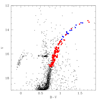
Figure 1: The $V,B-V$ CMD of NGC 1851 with stars selected for the present study indicated by large red filled circles (GIRAFFE targets) and large blue squares (UVES targets).

Initially, 124 member stars (according to the radial velocity RV, see below) were targeted with GIRAFFE fibres and 14 stars with the fibre-fed UVES spectrograph (Red Arm, with spectral range from 4800 to 6800 Åand R=45000); 10 stars were observed with both instruments.

Table 1: Log of FLAMES observations for NGC 1851

Date	UT	exp.	grating	seeing	airmass
		(sec)
Apr. 09, 2010	23:53:06.585	2880	HR11	0.82	1.355
Apr. 11, 2010	00:21:43.120	2880	HR11	0.67	1.514
Aug. 05, 2010	09:13:30.637	2880	HR11	1.02	1.533
Aug. 26, 2010	07:57:12.771	2880	HR13	1.21	1.497
Aug. 26, 2010	08:47:34.969	2880	HR13	1.11	1.278
Sep. 01, 2010	08:00:05.991	2880	HR13	1.78	1.368
Sep. 02, 2010	07:41:33.444	2880	HR13	1.35	1.435

We used the 1-D, wavelength calibrated spectra as reduced by the dedicated ESO Giraffe pipeline to derive RVs using the IRAF task FXCORR, with appropriate templates, while the RVs of the stars observed with UVES were derived with the IRAF task RVIDLINES.

Three stars with GIRAFFE spectra and one with UVES spectra were successively dropped from the sample, because of unreliable photometry and/or spectra. Hence our final sample for NGC 1851 consists in 124 RGB stars, the largest set ever observed with high resolution spectroscopy in this cluster. Coordinates, magnitudes and heliocentric RVs are shown in Tab. LABEL:t:coo18 (the full table is only available in electronic form at CDS).

3 Atmospheric parameters and abundance analysis

We derived the atmospheric parameters and abundances using the same technique adopted for the other GCs targeted by our FLAMES survey. In particular, since we think we have detected a small metallicity spread in NGC 1851, the reference paper where the tools are described in detail is the analysis of M 54 (Carretta et al. 2010e), although in that case the spread in [Fe/H] is much larger. Therefore, only a few points of the analysis will be summarised here.

As usual, we derived first estimates of $T_{\rm eff}$ (from $V-K$ colours) and bolometric corrections using the calibrations of Alonso et al. (1999, 2001). Subsequently, we refined the $T_{\rm eff}$ estimates for the stars using a relation between $T_{\rm eff}$ and $K$ magnitudes. Gravities were obtained from stellar masses and radii, these last derived from luminosities and temperatures. Within this procedure, the reddening and the distance modulus for NGC 1851 were taken from the Harris (1996) catalogue (2011 update), and we adopted masses of 0.85 M_⊙ for all stars and $M_{\rm bol,\odot}=4.75$ as the bolometric magnitude for the Sun, as in our previous studies.

The abundance analysis is mainly based on equivalent widths ($EW$s). Those measured on GIRAFFE spectra were corrected to the system given by UVES spectra. Values of the microturbulent velocities $v_{t}$ were obtained by eliminating trends between Fe i abundances and expected line strength (Magain 1984). Finally, we interpolated models with the appropriate atmospheric parameters and whose abundances matched those derived from Fe i lines within the Kurucz (1993) grid of model atmospheres (with the option for overshooting on). The adopted atmospheric parameters and iron abundances are listed in Tab. LABEL:t:atmpar18.

The procedure for error estimates is the same as in Carretta et al. (2010e) and results are given in the Appendix for UVES and GIRAFFE observations in Tab. 14 and Tab. 15, respectively.

As in our previous papers, oxygen abundances are obtained from the forbidden [O i] lines at 6300.3 and 6363.8 Å, after cleaning the former from telluric lines as described in Carretta et al. (2007c). The prescription by Gratton et al. (1999) were adopted to correct the derived Na abundances for non-LTE effects (from the 5682-88 and 6154-60 Å doublets). Abundances of Al (from the 6696-99 Å doublet) and Mg are derived as in Carretta et al. (2009b). The abundances of these proton capture elements for individual stars are listed in Tab. LABEL:t:proton18.

The observed $\alpha-$elements in the present study are Mg (reported among proton-capture elements), Si, Ca, and Ti. The abundances for these elements were derived for stars with either UVES or GIRAFFE spectra (see Tab. LABEL:t:alpha18). For the first ones, we measured Ti abundances from both neutral and singly ionised species, due to the large spectral coverage of UVES spectra.

Concerning the Fe-peak elements, we measured lines of Sc ii, V i, Cr i, Co i, and Ni i for stars with GIRAFFE and UVES spectra and additionally of Mn i and Cu i for stars with UVES spectra. Whenever relevant (e.g. Sc, V, Mn, Co), we applied corrections due to the hyperfine structure (see Gratton et al. 2003 for references). For Cu i we used the transition at 5105 Å, which we synthesised using a line list kindly provided by J. Sobeck in advance of publication. The line list takes into account both isotopic structure and hyperfine splitting. We adopted the solar isotopic ratio of 69% ⁶³Cu and 31% ⁶⁵Cu. Abundances of Fe-peak elements for individual stars are reported in Tab. LABEL:t:fegroup18.

We derived the concentration of several neutron capture elements, mostly from UVES spectra. We measured the abundances of Y ii, Zr ii, Ba ii, La ii, Ce ii, Nd ii, Eu ii, and Dy ii through a combination of spectral synthesis and EW measurements. A few details follow for each element.

Y ii:

We used four transitions (at 4883, 5085, 5200, 5206 Å). They were synthesised using the same atomic parameters as listed in Sneden et al. (2003). An example of the fit of the 4883 Å line for star 14080 is given in Fig. 2.

Zr ii:

The line at 5112 Å is the only clean usable line included in our spectral range. We adopted the $gf$ and excitation potential listed by Biemont et al. (1981).

Ba ii:

Four lines were used to estimate the abundance: 4934.1, 5853.7, 6141.7, and 6496.9 Å. We used spectral synthesis for the bluest line, since it is affected by considerable blending with a strong Fe line in the spectra under consideration. For the remaining lines, the abundance was measured through their EWs, because they are clean from blending for the stars of NGC 1851. The transition parameters adopted are from Sneden et al. (1996). An example of the fit of the 5853 Å line for star 14080 is given in Fig. 2. Even though we derived the abundance from EWs for this particular line, we chose it to display a synthesis to show that the Ba abundance from V10 for this particular star is not a good fit to our data (at least using our adopted atmospheric parameters). We note that abundances from synthesis and EW agree very well for the plotted line.

La ii:

We used four lines (4921.0, 4921.8, 5114.5 and 6262.3 Å). The three bluest ones were synthesized, as they have a not negligible hyperfine structure. Abundances from the other line were derived from EWs measurements. The transition parameters adopted are from Sneden et al. (2003). An example of the fit of the 5114.5 Å  line for star 14080 is given in Fig. 2.

Ce ii:

We used one line at 5274.3 Å. The transition parameters adopted are from Sneden et al. (2003). We assign a smaller weight to our Ce abundances, because of possible blending of this line.

Nd ii:

We used 9 lines for which we measured EWs (5092.8, 5130.6, 5165.1, 5212.4, 5234.2, 5249.6, 5293.2, 5311.5, and 5319.8 Å). The transition parameters adopted are from Sneden et al. (2003).

Eu ii:

We synthesised two spectral lines, at 6437.6 and 6645.1 Å. This technique was used because they are affected by considerable hyperfine splitting. The transition parameters adopted are from Sneden et al. (2003). An example of the fit of the 6645 Å line for star 14080 is given in Fig. 2.

Dy ii:

Abundance was derived from EW of the line at 5169.7 Å. The transition parameters adopted are from Sneden et al. (2003).

Figure 2: Examples of syntheses for lines due to four $n-$capture species in star 14080. Upper left side: syntheses for the Y ii line at 4883 Å, the abundances plotted are [Y/Fe]ii=0.1, 0.3 and 0.5 dex. Upper right side: as upper left for the Ba ii line at 5853.5 Å  for [Ba/Fe]ii=0.30,0.50 and 0.70 dex. Lower right side: as upper left for the Eu line at 6645.1 Å  for [Eu/Fe]ii=0.4, 0.6,0.8; lower left side: as for upper left for the La ii line 5114.5 Å  for [La/Fe]ii=0.2, 0.4 and 0.6  dex. For Y and Ba the solid lines indicate the values reported in V10 for this star.

Results are given in Tab. LABEL:t:neutron18 and Tab. LABEL:t:zrba18 for stars with UVES and GIRAFFE spectra, respectively. The averages of all measured elements with their $r.m.s.$ scatter are listed in Tab. 9.

Table 9: Mean abundances from UVES and GIRAFFE

Element	UVES	GIRAFFE
	n   avg   $rms$	n   avg   $rms$
$[$O/Fe$]$i	13 +0.04 0.25	86 $-$0.01 0.21
$[$Na/Fe$]$i	13 +0.26 0.25	120 +0.19 0.28
$[$Mg/Fe$]$i	13 +0.35 0.03	119 +0.38 0.04
$[$Al/Fe$]$i	13 +0.13 0.21
$[$Si/Fe$]$i	13 +0.38 0.03	120 +0.39 0.03
$[$Ca/Fe$]$i	13 +0.30 0.02	121 +0.33 0.04
$[$Sc/Fe$]$ii	13 $-$0.01 0.08	121 +0.03 0.06
$[$Ti/Fe$]$i	13 +0.17 0.07	118 +0.15 0.05
$[$Ti/Fe$]$ii	13 +0.17 0.05
$[$V/Fe$]$i	13 $-$0.06 0.09	116 $-$0.13 0.12
$[$Cr/Fe$]$i	13 $-$0.02 0.06	113 +0.05 0.11
$[$Mn/Fe$]$i	13 $-$0.34 0.08
$[$Fe/H$]$i	13 $-$1.18 0.07	121 $-$1.16 0.05
$[$Fe/H$]$ii	13 $-$1.14 0.12	101 $-$1.13 0.07
$[$Co/Fe$]$i	13 $-$0.24 0.06	49 $-$0.03 0.07
$[$Ni/Fe$]$i	13 $-$0.10 0.03	120 +0.02 0.07
$[$Cu/Fe$]$i	13 $-$0.46 0.07
$[$Y/Fe$]$ii	13 +0.27 0.15
$[$Zr/Fe$]$ii	13 +0.26 0.11
$[$Ba/Fe$]$ii	13 +0.48 0.26	101 +0.49 0.22
$[$La/Fe$]$ii	13 +0.23 0.17
$[$Ce/Fe$]$ii	13 +0.69 0.20
$[$Nd/Fe$]$ii	12 +0.67 0.15
$[$Eu/Fe$]$ii	13 +0.67 0.11
$[$Dy/Fe$]$ii	13 +0.67 0.12

4 Metallicity spread and stellar population components

4.1 Metallicity spread in NGC 1851

In Carretta et al. (2010c) we argued we detected a small but real metallicity spread in NGC 1851 by comparing observed abundances with internal errors. We deem that result robust because it rested on a statistically significant sample. NGC 1851 shows a much larger dispersion in [Fe/H] values when compared to other GCs of similar metal abundance, examined with the same instrumentation and technique of analysis (M4 and M5: see Fig. 3).

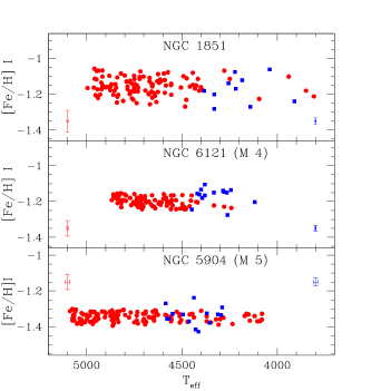
Figure 3: [Fe/H] ratios as a function of effective temperature for stars analysed in NGC 1851 (upper panel), M 4 (middle panel) and M 5 (lower panel), both from Carretta et al. 2009a,b). The filled red circles indicate stars with GIRAFFE spectra, the blue filled squares stars with UVES spectra. Error bars in the left and right side of the panels refer respectively to our GIRAFFE and UVES data and indicate star-to-star errors.

Apart from a larger scatter among the brighter stars observed with UVES (discussed in detail in Carretta et al. 2009c), the iron dispersion observed in M 4 and M 5 is compatible with internal errors associated to the analysis, 0.025 and 0.023 dex, respectively. However, if we try to fit the iron distribution in NGC 1851 using a Gaussian with FWHM equal to 0.024 dex (the average error from M 4 and M 5, Fig. 4) the plot clearly indicates the presence of a small intrinsic dispersion in the iron content that cannot be accounted for by internal errors alone.

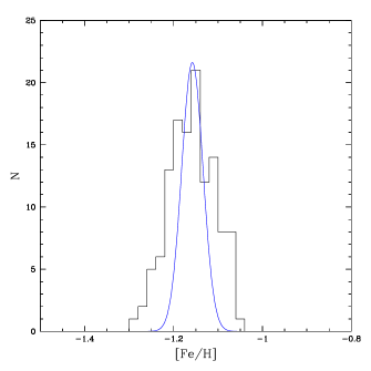
Figure 4: Histogram of [Fe/H] ratios for our NGC 1851 stars. For the gaussian curve we adopted as FWHM=0.024, that is the average standard deviation in [Fe/H] between the mono-metallic GCs M 4 (rms=0.025) and M 5 (rms=0.023, see Carretta et al. 2009c).

On the other hand, the comparison of the scatter in Fe abundances (Tab. 9) with the internal errors estimated in the Appendix shows that the observed dispersion in [Fe/H] i for NGC 1851 are statistically significant for stars with metallicity from UVES, as pointed out in Carretta et al. (2010c). In this case, internal errors are of the order of 0.03 dex, much lower than the observed scatter (0.07 dex). The case is less compelling for the abundances from GIRAFFE data, for which, we obtained an internal error on [Fe/H] (0.043 dex) not much lower than the observed scatter ($0.051\pm 0.005$ dex). However, putting together the highly significant result obtained from UVES spectra with the hint coming from GIRAFFE ones and the consideration that the observed scatter is much larger than for the similar clusters M4 and M5, we conclude in favour of a real dispersion in [Fe/H] values within NGC 1851.

A similar amount of intrinsic scatter was also found by Yong and Grundahl (2008). The eight stars observed in that study have an average [Fe/H]=$-1.268\pm 0.030$ with a 1$\sigma$ r.m.s. scatter of 0.084 dex. Although there is a small offset with respect to the present analysis (likely due to different temperature and $gf$ scales adopted), their study agrees with us on the reality of a small metallicity dispersion in NGC 1851. On the other hand, V10 did not find any scatter in [Fe/H] among their 15 stars.

Given the method used to derive atmospheric parameters for individual stars, a potential contamination by AGB stars in our sample could increase the observed scatter. This might occur in particular for the UVES sample, where most of the stars are brighter than the magnitude limit at which it is easy to discriminate AGB and RGB stars (see Fig. 1). From this diagram the AGB is clearly discernible from the RGB below $V\sim 14.5$ ($T_{\rm eff}\sim 4300$ K and $M_{V}\sim-1$). For fainter stars, we simply omitted AGB stars from our sample. For brighter stars, the two sequences do not appear any more distinct, because such bright AGB stars are $<50$ K warmer than first ascent RGB stars (this value is derived from the isochrone by Bertelli et al. 2008 at Z=0.001 and 12.6 Gyr). Our sample may then include some bright AGB stars. However, we believe that this is not a source of concern owing to several reasons. First, we expect very few AGB stars, since they are less than about 20% of the red giants: hence on 17 observed stars brighter than the limit we expect only about three AGB interlopers. Second, the errors produced in the analysis are small. In fact, even if we make an error of 0.2 $M_{\odot}$, by mistaking AGB stars for RGB stars, this translates into an error of 0.1 dex in $\log{g}$, all the other parameters being held fixed; and, as mentioned above, the errors made in the $T_{\rm eff}$ values are $<50$ K. Using the sensitivities listed in Tab. 15 and Tab. 14 in the Appendix, the gravity error would imply errors in the derived [Fe/H] ratio of $-0.003$ dex and $+0.012$ dex for GIRAFFE and UVES, respectively. Due to errors in temperature, bright AGBs confused in the RGB sample could appear up to be $0.04\div 0.06$ dex more metal-poor than the other stars. These effects are very small. Furthermore, we notice that the observed metallicity scatter is about constant over the whole temperature range, either including or not the temperature range where possible contamination by AGB stars exist (see Fig. 3).

Therefore, the observed spread seems real, and not due to a neglected contamination from AGB stars. This is corroborated by the good agreement we obtain, on average, between abundances based on neutral and singly ionised species (e.g. iron) that supports the atmospheric parameters we used, including surface gravities $\log{g}$. More in general, we do not attribute much weight to the small offset between the abundances of neutral and singly ionised iron, which is well within 1$\sigma$ r.m.s. scatter, thus hardly significant. The [Fe/H] ii abundances rest on only one-two lines for GIRAFFE spectra and bright stars (those observed with UVES) are also cooler, on average, hence more subject to possible NLTE effects. Anyway, we do not use [Fe/H] ii in any of our conclusions.

Finally, we stress that in the present analysis the observed spreads are only lower limits, owing to the particular way we derive the final temperatures, using a mean relation between T${}_{\rm eff}(V-K)$ and the $K$ magnitude along the RGB. While this technique allows us to have extremely small internal errors (see Carretta et al. 2007a for details), it also tends to slightly reduce any real metallicity spread along the RGB, leading us to adopt an effective temperature corresponding to a mean ridge line. Had we iteratively used slightly different temperature-magnitude relations for each component, we would have obtained not very different results, on average, the maximum additional difference in [Fe/H] amounting to less than 0.04 dex.

Anyway, on top of these results, the most striking evidence of a difference in the stellar populations on the RGB in NGC 1851 is the spatial distribution of the metal-rich (MR) and metal-poor (MP) components (Carretta et al. 2010c). We found there a clearcut evidence that stars more metal-poor than the cluster average ([Fe/H]$=-1.16$) are more centrally concentrated than more metal-rich stars, with a very high degree of confidence. There is something intrinsically different between the MR and MP populations in NGC 1851.

This finding bypasses any debate on the reality of radial distribution of SGB stars in the existing literature and was possible only owing to the large number of stars analysed in a very homogeneous way. This observation stimulated the working hypothesis proposed in Carretta et al. (2010c) that NGC 1851 might be the result of a merger of two originally distinct clusters, with a slightly different metallicity.

There are other differences between the MR and MP components, beside [Fe/H] and radial distribution, in the content of $\alpha-$capture and neutron-capture elements (see below). Moreover, in each individual component there is a well developed Na-O anticorrelation (Carretta et al. 2010c), which is the chief signature of a genuine globular cluster, according to Carretta et al. (2010a). Very recently, a very similar finding has been obtained for M 22 (Marino et al. 2011), which has several analogies with NGC 1851.

4.2 A cluster analysis approach to stellar components in NGC 1851

While the choice of the average [Fe/H] as separating value between the two populations is the simplest one, it is also arbitrary. To seek for a more objective criterion we exploit the main results obtained up to now for NGC 1851 (Carretta et al. 2010c): (i) there is a real (small) metallicity dispersion in the cluster, where (ii) the MP component is more centrally concentrated, and moreover (iii) the MR component shows a higher level of $s-$process elements. These observations suggest to use the run of [Fe/H] as a function of [Ba/H] as a population diagnostic to separate the two stellar components in NGC 1851. On this data, we performed a cluster analysis using the $k-$means algorithm (Steinhaus 1956; MacQueen 1967), as implemented in the $R$ statistical package (R Development Core Team, 2011), a system for statistical computation and graphics, freely available on-line. Two key features of $k-$means are:

• Euclidean distance is used as a metric and variance is used as a measure of cluster scatter. The various parameters used should be transformed before computing these distances, in order to weight them adequately. A sensible choice is to normalize them to the observational errors. In practice, as normalization factors we assumed errors of 0.04 and 0.20 dex for [Fe/H] and [Ba/H] respectively.

• The number of clusters $k$ is an input parameter: an inappropriate choice of $k$ may yield poor results. Given that the ratio between observed scatter of data and observational errors is not large, we adopted $k=2$. Of course, there may be more than two groups of stars in NGC 1851, but we wished to limit the number of hypothesis at this stage.

A key limitation of $k-$means is its cluster model. The concept is based on spherical clusters that are separable in a way so that the mean value converges towards the cluster center. The clusters are expected to be of similar population, so that the assignment to the nearest cluster center is the correct assignment. When the clusters have very different size, this may result in poor assignation of members to clusters. However, in the present case, we expect that most of the scatter within one cluster is due to observational errors, which are similar for the different clusters. We then considered the assumption of similar size for the different clusters acceptable. Of course, this does not mean that occasionally assignation of some member (that is, star) to a particular cluster is questionable.

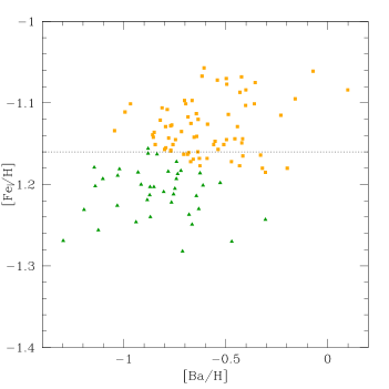
Figure 5: Diagnostic diagram [Fe/H] vs [Ba/H] for the stellar components in NGC 1851. The different symbols and colour coding show the results of the cluster analysis using Fe and Ba abundance as parameters (see text). Stars indicated with orange filled squares are attributed to the MR component; stars indicated with green filled triangles are assigned to the MP component. The dotted line indicates the average value [Fe/H]$=-1.16$ dex for NGC 1851 which we previously adopted as separating value.

The results are shown in Fig. 5, where the two components are indicated with different symbols and colours. We also superimpose a line indicating the average value [Fe/H]$=-1.16$ dex for NGC 1851, adopted by Carretta et al. (2010c) to separate the two components using only the metallicity.

Notice that 13 stars did not have Ba abundances because lacking of UVES or HR13 GIRAFFE spectra. For 10 stars it is easy to unambiguously assign a population simply according to the metallicity (most of them falling above [Fe/H]$=-1.10$ or below [Fe/H]$=-1.20$ dex). However, for three stars (28116, 33385, 40300) this is not possible and their status is currently uncertain.

The cluster analysis shows that the new components are similar to, but not exactly coincident with, those defined in Carretta et al. (2010c). The separation line is slightly slanted and not simply an average value, when accounting also for the enhanced level of Ba in the most metal-rich component. However, for simplicity, we continue to talk of MR and MP components. The main change is that the MP component decreases from 50% to 36% while the MR one increases to 64%. These fractions are now tantalisingly close to the fractions of stars observed on one hand on the faint SGB (45%) and the BHB (40%), and on the other hand on the bright SGB (55%) and RHB (60%, see Milone et al. 2008). This might suggest a tentative link according to the new population ratios, although this link should actually be confirmed by determination of abundances for SGB and HB stars.

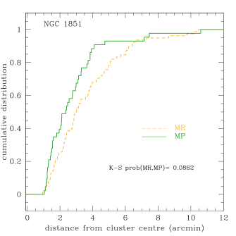
Figure 6: Cumulative distribution of radial distances for all stars in our sample, divided in MP (green solid line) and MR (dashed orange line) components.

Also with this new definition the MP component results to be more concentrated than the MR one to a reasonable level of confidence (see Fig. 6).

Milone et al. (2009) considered the issue of the radial distribution of the different populations in NGC 1851, claiming no difference between the two SGBs. Their sample is much more numerous than ours, and since their conclusion is apparently different, we re-examined their result. In their analysis, they considered three possible cases (labelled A, B and C), depending on the interpretation of the splitting of the SGB. Case A is for a simple age difference (about 1 Gyr); case B is for a combination of age differences (about 2 Gyr) and CNO abundance variations; and case C is for a difference only in the sum of CNO abundances. If we use as metrics for the comparison the Pearson correlation coefficient between the radius and the fraction of faint SGB stars, there is slightly more than 5% of probability that the correlation is random for cases A and B, while there is no clear difference for case C. Since they seems to prefer this last scenario, Milone et al. (2009) concluded that there is no difference in the radial distribution of the different populations of NGC 1851. However, much more could be said apropos. First, obviously lack of evidence is not evidence of lack. Second, in their data there is indeed some hint for a radial gradient, the faint SGB being more concentrated than the bright SGB. While the test considered above seems not strong enough to allow a conclusion at a high confidence level, other tests like the Kolmogorov-Smirnov one are more powerful in revealing differences among distributions, and would seem more appropriate in this context. While we have not at our disposal enough data to perform the Kolmogorov-Smirnov test on their data, we might use other metrics. For instance, we may compare the weighted averages of the three innermost and of the three outermost bins. Using this approach, we found differences of $0.11\pm 0.06$, $0.17\pm 0.07$, and $0.06\pm 0.06$ for cases A, B, and C. Summarizing, the lack of evidence claimed by Milone et al. (2009) is related to the statistics they used in their analysis and to the interpretative scenario they favour for the separation of NGC 1851 into two populations. The statistics used is likely not the most powerful one, and there is no strong spectroscopic evidence for a variation of the sum of CNO abundances in NGC 1851 (see also V10). We then think that their data cannot be used to conclude that there is no difference in the radial distributions of the different populations of NGC 1851.

4.3 Kinematics of stellar components in NGC 1851

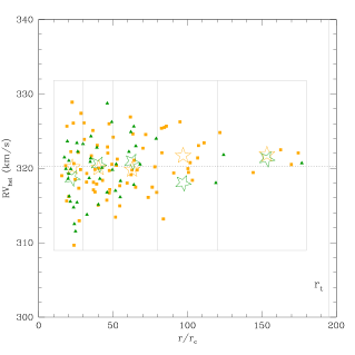
Figure 7: Distribution of radial velocities for all stars in our sample, divided in MP (filled greed triangles) and MR (filled orange squares) components. The x axis shows the distance from the cluster centre (in units of the core radius $r_{c}$). The larger symbols, also in green and orange, represent the average RV of the two sub-samples, computed in the boxes indicated in the figure. The dotted horizontal line represents the global average of the sample (320.26 km s^-1, with a rms of 3.74) and the vertical line indicates the tidal radius. The average RVs at the various distances are given in Table 10.

In principle, if the MP and MR components come from two distinct sub-units they could also have different kinematics, showing up in their velocity distribution. However, we found no significant differences: the velocity dispersion increases from the outskirts towards the cluster centre (see Fig. 7 and Tab. 10) but for the MR and MP the pattern is similar, apart from the different concentration of stars in the two components.

Table 10: Average RVs for MP and MR stars at different distances from the cluster centre

Dist.	$<RV(MR)>$	rms	Nr.	$<RV(MP)>$	rms	Nr.
(in $r_{c}$)	(km s${}^{-1})$		MR	(km s-1)		MP
10-30	320.16	5.25	16	318.67	3.90	16
30-50	320.05	3.26	23	320.55	4.25	13
50-80	319.82	3.51	20	320.91	3.30	11
80-120	321.70	3.59	14	318.04	0.00	1
$>$120	321.86	2.05	5	321.25	0.78	2

Given the limitations of our sample, we cannot tell if this is due to insufficient data or it has some real physical meaning. We only notice that if the merger is recent, there could be only a small dynamical effect, because after the merging the cluster would not be relaxed, and there might be no energy equipartition between the different populations. The merging between the two putative clusters could well be an event occurred only a few Gyrs ago: the relaxation time at the half mass radius (and we sampled a region external to this radius) is about 0.7 Gyr (Harris 1996), and a full cluster relaxation does require some 2-3 relaxation times. In the framework outlined in Carretta et al. (2010a) for the formation model of globular clusters, the only constraint is that the merger between the two clusters must have occurred before their host dSph galaxy merged with our Galaxy. However, we do not know when this possible interaction happened. If some debris of this putative dSph still exist (as suggested by several authors, e.g. Carballo-Bello et al. 2010, Olszewski et al. 2009) then the event could be rather recent. More data and detailed dynamical modelling would be required; however, this is beyond the purpose of the present work, which is focused on the chemical tagging.

5 The complex nucleosynthesis in NGC 1851

5.1 Nucleosynthesis in cluster environment: the proton capture elements

The pattern of observed (anti)correlations among light elements like C, N, O, F, Na, Mg, Al, Si requires a specific chain of events, restricted to the proto-cluster environment (see e.g. Gratton et al. 2004). Unavoidable requirement for a GC is the presence of a first generation of stars providing at their death the material, processed through proton-capture reaction in H-burning at high temperature, that participated to the formation of the second stellar generation(s) with modified chemical composition.

These considerations, together with the existence of the Na-O anticorrelation among stars of each metallicity component on the RGB of NGC 1851, support the merger of two clusters as a viable origin to explain the observed characteristics of this cluster. We will now examine whether this simple working hypothesis is robust against our revised classification (Sect. 4.2) of stellar populations and the full set of abundances derived for NGC 1851.

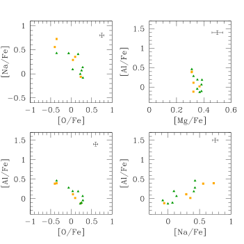
Figure 8: Na-O (top-left panel), Mg-Al (top-right panel), Al-O (bottom-left panel) anticorrelation, and Na-Al correlation (bottom-right panel) for stars with UVES spectra in NGC 1851. Green triangles and orange squares indicate stars of the MP and MR component, respectively. Error bars are star-to-star errors.

The (anti)correlations among proton-capture elements in NGC 1851 are summarised in Fig. 8 for stars with UVES spectra, from which the whole set of Na, O, Mg, Al abundances is available. NGC 1851 shows a moderate Na-O anticorrelation, and a well defined Na-Al correlation, with a not extremely high production of Al. In Fig. 8 there is a hint that stars of the MR component may reach more extreme processing than stars of the MP component, but this sample is limited.

The global Na-O anticorrelation presents stars well mixed over all the metallicity range, and its extension (as measured by the interquartile range IQR[O/Na]=0.693) well fits the strong correlations with the total cluster mass (using the absolute visual magnitude $M_{V}=-8.33$ as a proxy) and with the maximum temperature along the HB derived and widely discussed in Carretta et al.(2010a) (see Fig. 9).

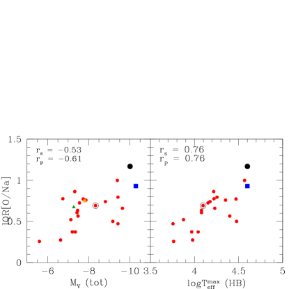
Figure 9: Interquartile range of the [O/Na] ratio, IQR[O/Na], for the stars in NGC 1851 as a function of the total absolute visual magnitude (left panel) and of the maximum temperature reached by HB stars (mainly from Recio-Blanco et al. 2006, right panel). NGC 1851 is indicated by a circled filled point. The large black filled circle and blue square are for M 54 and $\omega$ Cen, respectively. The IQR values come from Carretta et al. (2010b) and from data by Johnson and Pilachowski (2010), respectively, and maximum temperatures estimated by Cassisi (2011, private communication). The Spearman rank correlation coefficient ($r_{s}$) and the linear regression Pearson’s correlation coefficient ($r_{p}$) are listed in each panel. In the left panel, the green triangle and the orange square indicate the values relative to the MP and MR components in NGC 1851 (see text).

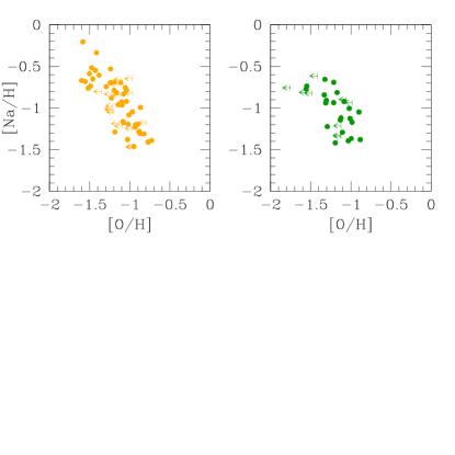
Figure 10: Na-O anticorrelation for stars of the MR (left panel) and of the MP (right panel) component in NGC 1851.

The cluster analysis, based only on Fe and Ba abundances, separates stars of NGC 1851 in two sub-groups, each one presenting a clean Na-O anticorrelation. The anticorrelation is slightly more extended for the MR component (IQR[O/Na]=0.750) than for the MP one (IQR[O/Na]=0.674) (see Fig. 10). As an exercise, we tentatively distributed the total $M_{V}=-8.33$ of NGC 1851 over the two MR and MP components by using the number of the RHB (191) and of BHB stars (116), respectively, adopted by Gratton et al. (2010b) in their study of the HB in this and other GCs. The resulting values are $M_{V}=-7.81$ and $M_{V}=-7.27$ for the MR and MP groups, respectively. When coupled with the IQR values derived above, the two components of NGC 1851 nicely fit the overall relation between $M_{V}$ and IQR[O/Na] (green and orange symbols in the left panel of Fig. 9). This supports the idea that the two components in NGC 1851, selected using independent parameters (Fe, Ba), do behave as two individual GCs with slightly different total masses.

To further support this evidence, we used the Strömgren photometry by Grundahl (available through the database used by Calamida et al. 2007) to plot the stars of the P, I and E components in NGC 1851. The definition of the primordial (P), intermediate (I) and extreme (E) population in a cluster, based on Na and O abundances, is illustrated in Carretta et al. (2009a), where we showed how the P (Na-poor, O-rich) stars of the first generation lie on a narrow strip to the blue of the RGB, while the I+E second generation stars are spread out to the red in a Strömgren $u,u-b$ CMD. The $u,u-b$ CMD is a good plane where to look for this segregation, since the splitting is due to the effect of the absorption by NH in the wavelength range sampled by near-UV bandpasses such as the Johnson $U$ (e.g. Marino et al. 2008), the Strömgren $u$ or even the Sloan $u$ bandpass (see Lardo et al. 2011), as also discussed by Sbordone et al. (2011) and Carretta et al. (2011). We show in Fig. 11 the results for NGC 1851 using stars observed both by us and Grundahl: in each metallicity group, the three components are nicely distributed along the RGB as if each group were an individual GC.

The fraction of stars in the primordial, intermediate and extreme components for NGC 1851 and the two MR and MP metallicity components are listed in Table 11. Even considering the rather large errors from the Poisson statistics, the fraction of primordial stars in the MR component appears to be smaller than the P fraction in the MP component. These fractions are computed using stars with both O and Na abundances (Carretta et al. 2009a). If we use only Na abundances, regardless of O abundance (this by definition allows us only to separate first and second generation stars, since it is a criterion “blind” to the separation between I and E stars) then the fractions of primordial stars in the MR and MP components are still rather different: $21\pm 5\%$ and $40\pm 10\%$, respectively.

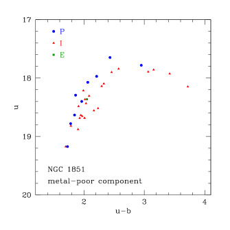
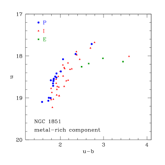
Figure 11: Strömgren $u,u-b$ CMD for stars of the MP (upper panel) and of the MR component (lower panel) in NGC 1851. In each panel, blue filled circles represent the P (first generation) group, the red triangles the intermediate I group, and the green squares the extreme E group of second generation stars.

Table 11: Number of stars with both Na and O abundances and fraction of the Primordial, Intermediate, and Extreme components

CASE	N.stars	fraction	fraction	fraction
	(O,Na)	P	I	E
	GIR.+UVES	component	component	component
NGC 1851 all	95	$31\pm\leavevmode\nobreak\ 6$	$63\pm\leavevmode\nobreak\ 8$	$6\pm 3$
NGC 1851 MR	61	$20\pm\leavevmode\nobreak\ 6$	$72\pm\leavevmode\nobreak\ 11$	$8\pm 4$
NGC 1851 MP	34	$44\pm\leavevmode\nobreak\ 11$	$53\pm\leavevmode\nobreak\ 12$	$3\pm 3$

Fig. 12 shows the location of a slight change of the mean value of O and Na abundances, just at the level of the bump on the RGB. We remind the reader that our interpretation (the change is caused by the mix of first and second generation stars, each generation with its own slightly different He content, see Salaris et al. 2006 and Bragaglia et al. 2010) is based on the observation that the ratios [Na/Fe] and [O/Fe] run essentially flat as a function of luminosity in field stars (Gratton et al. 2000). While lighter species (such as Li, C and N) can be mixed up, the ON and NeNa cycles require higher temperatures: they are cycled in the inner layers of the H-burning shell that cannot be reached by the extra-mixing processes even after the RGB-bump. In the case of NGC 1851, where probably we could see the result of two distinct clusters, each with its own Na-O anticorrelation and P,I, and E components, we expect a further smearing of the bump in the RGB luminosity function.

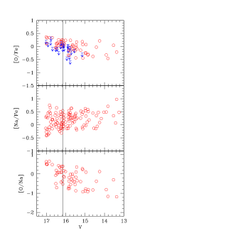
Figure 12: [O/Fe], [Na/Fe] and [O/Na] ratios (upper, middle, and lower panel, respectively) in RGB stars of NGC 1851 as a function of $V$ magnitude. The RGB-bump luminosity level is indicated by a solid line. Upper limits in O are indicated by arrows.

Finally, we checked the other elements participating to the proton-capture reactions, namely Mg and Si, using the large sample of stars with homogeneous abundances from GIRAFFE spectra. In NGC 1851 (Fig. 13) the abundances of Mg are depleted as O is depleted and Na is enhanced, while the opposite happens for Si. The last occurrence is probably due to the leakage from the Mg-Al cycle on Si, first discovered by Yong et al. (2005) in NGC 6752 and then found by Carretta et al. (2009b) in stars of several clusters, although only in the small samples of RGB stars with UVES spectra. This is the first time that these relations involving Si are observed in a very large sample of stars in an individual cluster. The large statistics (85 stars with Mg, Si and O; about 120 stars with Mg, Si and Na) makes all the (anti)correlations in Fig. 13 robust to a high level of confidence. Although the internal errors are not negligible and the amount of variations in [Si/Fe] abundance ratios is not dramatic (about 0.1-0.15 dex), these relations tell us that at least part of the material from which the second generation stars formed was processed at a temperature exceeding $\sim 65$ million K. This is the threshold for which the reaction producing ²⁸Si becomes effective in the Mg-Al cycle (Arnould et al. 1999).

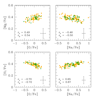
Figure 13: Top panels: [Mg/Fe] ratios as a function of [O/Fe] and [Na/Fe] for stars in NGC 1851 with GIRAFFE spectra. Bottom panels: [Si/Fe] ratios as a function of [O/Fe] and [Na/Fe]. In each panel the internal error bars and the Spearman rank and the Pearson linear regression coefficients are indicated. Stars are color coded according to their metallicity: green triangles for MP stars and orange squares for MR stars.

Separating the sample in the MR and MP components, the relations of Fig. 13 still hold in each sub-group.

5.2 Nucleosynthesis from massive stars: $\alpha-$elements

The elements involved in $\alpha-$capture reaction are the main signature of nucleosynthesis in massive stars, ending their lives as core-collapse supernovae. Of course, here we are considering the level of primordial enrichment of the gas from which the first stellar generation formed in the cluster. Subsequently, the abundance of some elements, like Mg, and Si may be modified by proton-capture reactions, as discussed in the previous section. Instead, no change should be observed for heavier elements, e.g. Ca, between multiple generations in a GC. The issue of chemical enrichment from massive stars has recently received new interest after the proposal by Lee et al. (2009b) that chemical pollution by type II SNe might be discerned in GCs hosting multiple populations.

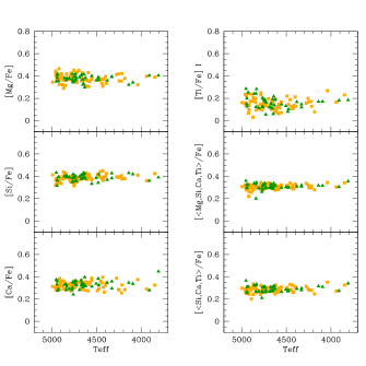
Figure 14: Run of the abundance ratios of Mg, Si, Ca (left panels), Ti i (upper right panel) and two averages for the $\alpha-$elements (last right panels) for stars in NGC 1851 with GIRAFFE spectra. In each panel the color coding is as in Fig. 13.

In Fig. 14 we show the run of $\alpha-$elements in NGC 1851 as a function of the temperature, using the large sample of stars with homogeneous abundances from GIRAFFE spectra. The mean overabundance is quite normal (Tab. 9) for cluster stars and the small observed scatter for Mg and Si is compatible with the Mg-Al cycle producing only small changes to the primordial level of Mg and Si, despite the noted anticorrelations and correlations discussed in the previous Section. No distinct trend is observed as a function of either effective temperature or metallicity, as evident by the adopted color coding.

However, the result is quite different if we plot the ratio with respect to the H abundance, as in Fig. 15: the absolute level of $\alpha-$elements is larger in the MR component of NGC 1851 than in the MP component. The evidence is somehow reduced for the case of Ti i but is very clear for Mg, Si, Ca.

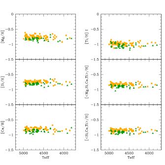
Figure 15: As in Fig. 14 but with element ratios all referred to H. The color coding is as in the previous Figure.

To put the comparison on a more quantitative ground, we list in Table 12 the average ratios measured for the MP and MR components separately, using both the [el/Fe] and [el/H] abundance ratios. The value of the variable $t$ for the t-test is also listed in the Table and it is used to assess whether the two averages are statistically different from each other. We found that while the [el/Fe] mean values cannot be statistically distinguished, the difference is significant with a high level of confidence when we compare the average [el/H] ratios between the two components.

Table 12: Mean abundances from GIRAFFE spectra for stars in the MR and MP component of NGC 1851

Element	MP component	MR component	t
	n   avg   $rms$	n   avg   $rms$
$[$Mg/Fe$]$i	39 +0.376 0.030	77 +0.378 0.037	0.21
$[$Si/Fe$]$i	40 +0.389 0.028	77 +0.384 0.029	1.00
$[$Ca/Fe$]$i	40 +0.329 0.038	78 +0.326 0.033	0.48
$[$Ti/Fe$]$i	39 +0.160 0.055	77 +0.151 0.048	0.94
$[$Sc/Fe$]$i	40 +0.025 0.059	78 +0.029 0.057	0.38
$[$V/Fe$]$i	38 $-$0.125 0.131	75 $-$0.127 0.109	0.08
$[$Cr/Fe$]$i	38 +0.023 0.110	72 +0.064 0.114	1.83
$[$Co/Fe$]$i	15 $-$0.027 0.073	32 $-$0.020 0.071	0.28
$[$Ni/Fe$]$i	40 +0.016 0.078	77 +0.019 0.065	0.24
$[$Ba/Fe$]$ii	32 +0.395 0.238	69 +0.538 0.203	2.94
$[$Mg/H$]$i	39 $-$0.828 0.047	77 $-$0.754 0.057	7.39
$[$Si/H$]$i	40 $-$0.816 0.045	77 $-$0.748 0.045	7.74
$[$Ca/H$]$i	40 $-$0.876 0.049	78 $-$0.807 0.047	7.41
$[$Ti/H$]$i	39 $-$1.045 0.063	77 $-$0.982 0.053	5.36
$[$Sc/H$]$i	40 $-$1.181 0.078	78 $-$1.104 0.076	5.14
$[$V/H$]$i	38 $-$1.330 0.132	75 $-$1.256 0.107	2.96
$[$Cr/H$]$i	38 $-$1.183 0.113	72 $-$1.069 0.129	4.79
$[$Co/H$]$i	15 $-$1.231 0.085	32 $-$1.149 0.076	3.21
$[$Ni/H$]$i	40 $-$1.190 0.094	77 $-$1.113 0.075	4.46
$[$Ba/H$]$ii	32 $-$0.809 0.241	69 $-$0.599 0.206	4.25

Thus, the metal-rich component in NGC 1851 also shows a higher level of $\alpha-$elements typically produced in core-collapse SNe.

In summary, these results are clearly telling us that the observed differences in the primordial chemical composition between the MP and MR components in NGC 1851 are due to core-collapse SNe and not to type Ia SNe, since the $\alpha-$elements track the Fe abundance and there is no significant difference in the [$\alpha$/Fe] ratios between the two populations.

What happens to the (anti) correlations between Mg, Si and Na, O seen in the previous section? We plot again in Fig. 16 the stars of Fig. 13, color coded as usual, but this time we use the [el/H] ratios.

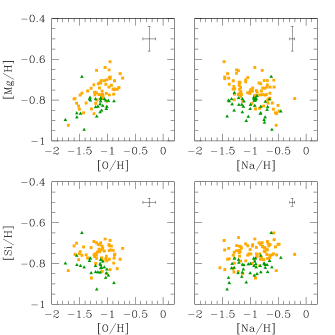
Figure 16: Top panels: [Mg/H] ratios as a function of [O/H] and [Na/H] for stars in NGC 1851 with GIRAFFE spectra. Bottom panels: [Si/H] ratios as a function of [O/H] and [Na/H]. In each panel the internal error bars are indicated. Stars are color coded according to their metallicity as in previous figures.

From this figure it is clear that the relations between elements involved in proton-capture reactions still hold, but they hold for each metallicity component separately: the only difference is that the level is shifted toward higher values for the MR component. The existence of these neat (anti)correlation in each metallicity group again supports two originally distinct GCs: for what we know at present, this kind of trends among light elements requires a precise chain of events and a nucleosynthesis only possible in a GC formation scenario (see Carretta et al. 2010a).

Anyway, whatever the interpretation is, we confirm that a difference of [Ca/H] does exist in NGC 1851. This difference was claimed by Lee et al. (2009b) from the observed spread in their $hk$ index. A more detailed comparison between spectroscopic and photometric results will be discussed below; however, as anticipated in Carretta et al. (2010c, their Fig.4) using Strömgren photometry, stars along the RGB in NGC 1851 are not segregated in metallicity [Fe/H], or [Ca/H], but only according to their belonging to the first or second stellar generation. There is little doubt that a spread of Ca is found in NGC 1851, but we found that its mean level only correlates with [Fe/H] and not with [Na/O].

Our simple interpretation (the merger of two distinct clusters formed within a large parent system) offers the advantage of explaining the observation in this peculiar cluster, and at the same time to account for other GCs where a spread of [Ca/H] values is excluded by high resolution spectroscopy (such as M 4, NGC 6752 and other GCs with no metallicity spread, see Carretta et al. 2010d).

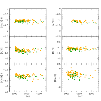
Figure 17: Run of the abundance ratios of Fe-group elements Sc ii, V, Cr, Co and Ni and of the neutron-capture element Ba ii in stars of NGC 1851 with GIRAFFE spectra. All abundance ratios are plotted with respect to H. The color coding used in previous figures is adopted.

The elements heavier than Ti, in particular the Fe-group elements (listed in Tab. LABEL:t:fegroup18), simply track the run of [Fe/H] in NGC 1851, hence are slightly enhanced in the metal-rich component (Fig. 17). Again, the difference between average values for the MR and MP components are statistically significant when the [el/H] ratios are used (Table 12).

5.3 Nucleosynthesis from less massive stars: neutron capture elements

5.3.1 $s-$ and $r-$process contributions

Neutron capture elements can be produced by both slow $s-$process, and by rapid $r-$process, where slow and rapid is for the $n-$capture with respect to the $\beta-$decay. The $r-$process is active in (some?) core collapse SNe, while the $s-$process is mainly active in the thermally pulsing phase of intermediate-low mass stars (main component), although the light elements might also be produced in massive stars (weak component). Hence, they have very different timescales. Both $r-$ and $s-$processes likely contributed to make the $n-$capture elements observed in NGC 1851. To estimate their relative importance, we compared the abundances of elements that in the Sun are mainly produced by the $s-$ and $r-$process. In practice (see also Carretta et al. 2010c), we considered the abundances of Ba and La as representative of $s-$process elements, and Eu to represent the contribution of the $r-$process. In the solar system the $r-$fraction of Eu is estimated to be more than 97%, while it is $<40$% for the other elements (for instance, it is $\sim 18$% for Ba, see e.g. Simmerer et al. 2004).

The run of the [Ba/Eu] ratio with [Fe/H] in NGC 1851 is shown in Fig. 18. As a comparison, we also plotted the values available for two other GCs, well known to have a large difference in the abundance of neutron capture elements (notably, those that in the Sun are mainly produced by $s-$process): M 4 (Ivans et al. 1999) and M 5 (Ivans et al. 2001). The range in [Ba/Eu] spanned by stars in NGC 1851 is large: about 0.80 dex, with 0.25 dex $r.m.s.$ scatter. There are stars with [Ba/Eu] as high as that of M 4, whereas others have a ratio as low as that of M 5 ones.

In metal-poor stars of NGC 1851 the $s/r$ ratio is lower than solar by about 0.2 dex. It may be reproduced by assuming that about 1/3 of Ba is made by the $r-$process, and the rest by the $s-$process. An even larger fraction of other elements that in the Sun are mainly due to the $s-$process (like e.g. Y and Zr) is likely due to the $r-$process in the MP component of NGC 1851. Over the metallicity range of NGC 1851, however, there seems to be a trend for increasing Ba, La and Ce with respect to Eu as metallicity increases. For the MR component, [Ba/Eu] is roughly solar. This is consistent with $\sim 4/5$ of the Ba of the MR component being due the $s-$process. In this case, the $s-$process dominates also for other elements, including Y and Zr.

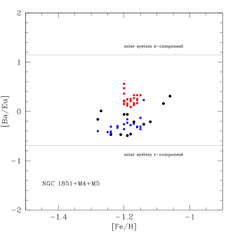
Figure 18: Ratios [$s$/$r$] in stars of NGC 1851 (black filled circles), M 4 (red squares, from Ivans et al. 1999) and M 5 (Ivans et al. 2001, blue squares). Ba and Eu are assumed as representative of the level of $s$ and $r-$process elements, respectively.

5.3.2 Light and heavy s-elements

Abundances of heavy elements might allow also to calculate the heavy (second peak) to light (first peak) $s$-process elements ratios for the stars in the sample. This ratio is important, since it can provide insight into the timescales of enrichment and the mechanisms responsible for it. In general, while it must be kept in mind that the neutron-density at the site of the $s-$process does in fact control it, for a given neutron-density (and metallicity) the heavy-to-light elements ratio does depend mostly on the stellar mass, with lower-mass stars ($\sim$1.5-2 M_⊙) undergoing a larger number of thermal pulses than $\sim$3 M_⊙ stars (Travaglio et al. 2004). In fact, the main neutron source for the mass range under consideration (1.5-3 M_⊙) is indeed the ¹³C($\alpha$,n)¹⁶O, whose sensitivity to temperature is rather moderate, making the neutron-flux very similar over the mass range. A high heavy-to-light ratio should then be related to a long timescale (even though overall metallicity must also be taken into consideration).

In order to obtain a meaningful evaluation of the heavy-to-light $s-$process ratio, the $r$-process contribution must be subtracted from the abundances of the heavy elements. To this aim, we used the following approach. We started by considering the solar $s-$ and $r-$ fractions listed in Simmerer et al. (2004) for Y, Zr, Ba, La, and Eu. We then assumed that the abundance ratios among different elements with similar atomic weight produced by the $r-$ and $s-$process are identical to the $r-$ and $s-$components measured in the Sun for all our sample stars; e.g., we have $\log{N_{\rm Eu_{s}}}/\log{N_{\rm Ba_{s}}}=$[$log{N_{\rm Eu_{s}}}/\log{N_{\rm Ba_{s}}}$]_⊙. This is a reasonable assumption, since these elements are close to each other in the nucleosynthesis chain. On this basis, we derived the $s-$ and $r-$ contribution for Eu and Ba for all stars. We then assumed that the $r-$process contribution for all elements scales proportionally (that is, we assumed a universal solar scaled $r-$process). This allows to determine the $r-$contribution for all elements in all stars. We subtracted this contribution to the abundances of all $n-$capture elements: the residual represents our best guess for the $s$-process contribution for each element in each star. This method provides reliable results insofar the $s-$contribution dominates over the $r-$one. Otherwise, results are quite unstable, depending heavily on observational errors.

To reduce this concern, we took the average of Y_s and Zr_s to represent the light $s$-process elements and Ba_s and La_s for the heavy ones. Note that for a few stars the estimated $r-$component for Y and La accounted for the entire measured abundances for these elements (stars involved are # 14080 and 43466 for both Y and La, and # 39801 only for Y). In such cases we only used Ba_s for heavy-$s$ and Zr_s for light-$s$. The remaining elements were not used either because we conservatively deemed our abundances not accurate enough (Ce) or because the large $r-$contribution makes results unreliable. Plots for the behaviour of the ratio of heavy-to-light $s-$process elements as a function of [Fe/H], measured Ba and Eu abundances ([Ba/Fe] and [Eu/Fe]) and [Ba/Fe]_s are shown in Fig. 19.

Closed and open symbols are for the metal rich and the metal poor population respectively. The large scatter among the metal-poor population is expected, since the $r-$contribution is typically large. In the metal-rich stars, for which results are more reliable, the [hs/ls] ratios are typically quite high . This suggests a contribution by low-mass AGB stars (M$\sim$1.5-3 M_⊙), at least for what concerns the high-metallicity population. However, it is unlikely that stars at the very lower end of this mass range (M$<2$M_⊙) have played a too large role in the chemical evolution of NGC 1851. In fact, these small mass stars do not deplete O; a large contribution by these stars would have diluted and even erased the Na-O anti-correlation. To maintain the Na-O anticorrelation, the contribution of the AGB stars that do not undergo HBB must be small with respect to those that do it. As an exercise, we calculated the amount of mass ejected by small mass AGB (not undergoing HBB), and by more massive ones (undergoing HBB), assuming a Salpeter IMF. We found that adopting a threshold for HBB of M=3 M_⊙, then only stars with M$>$2.2 M_⊙ could contribute to the second generation of NGC 1851, else the Na-O anticorrelation would be cancelled. Of course, this is a schematic approach: there are likely stars which both experienced HBB and thermal pulses. However, the qualitative argument that the contribution by low mass stars should be small is still valid.

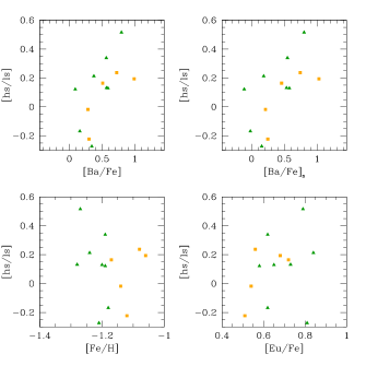
Figure 19: [hs/ls] as function of [Fe/H], total Ba and Eu abundances and Ba $s-$component abundance[Ba/Fe]_s. Closed and open symbols refer to the MR and MP components, respectively

It is interesting to note that recently, D’Orazi et al. (2011) used a similar approach to study the pattern of heavy elements in $\omega$ Cen. They found that this requires AGB stars even more massive than those here considered as the site for the $s-$process observed in that cluster.

5.3.3 Correlations between $n-$capture and $p-$capture element abundances

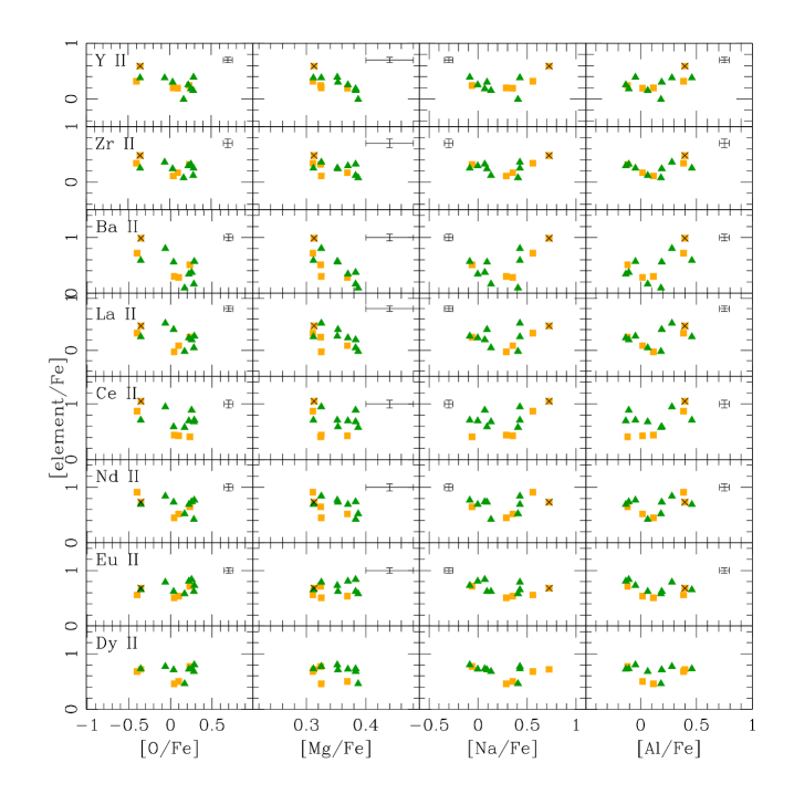
Figure 20: Abundance ratios of neutron capture elements in stars with UVES spectra, as a function of the proton capture elements O, Mg, Na, and Al. Stars are separated in MR and MP components as in previous figures. The star 32903 is indicated by a cross superimposed to the symbol. Error bars indicate internal errors.

Figure 21: [Ba/Fe] ratios as a function of [Na/O] for stars in NGC 1851 with GIRAFFE spectra, separated according to their sub-population. The Spearman rank coefficient $r_{s}$ and the Pearson linear regression coefficient $r_{p}$ are indicated for the whole sample and for both sub-populations.

Table 13: Pearson’s correlation coefficients, degree of freedom d.o.f., and level of significance for relations of neutron-capture vs proton-capture elements

element	all	MP	MR
	stars
Y ii vs O	0.61 11 95-98%	0.47 6 $<$90%	0.73 3 $<$90%
Y ii vs Mg	0.71 11 99%	0.83 6 99%	0.56 3 $<$90%
Y ii vs Na	0.33 11 $<$90%	0.11 6 $<$90%	0.72 3 $<$90%
Y ii vs Al	0.47 11 $<$90%	0.25 6 $<$90%	0.73 3 $<$90%
Zr ii vs O	0.47 11 $<$90%	0.24 6 $<$90%	0.61 3 $<$90%
Zr ii vs Mg	0.54 11 90-95%	0.51 6 $<$90%	0.59 3 $<$90%
Zr ii vs Na	0.25 11 $<$90%	0.14 6 $<$90%	0.46 3 $<$90%
Zr ii vs Al	0.24 11 $<$90%	0.10 6 $<$90%	0.55 3 $<$90%
Ba ii vs O	0.69 11 99%	0.56 6 $<$90%	0.78 3 $<$90%
Ba ii vs Mg	0.78 11 99%	0.86 6 99%	0.70 3 $<$90%
Ba ii vs Na	0.44 11 $<$90%	0.12 6 $<$90%	0.64 3 $<$90%
Ba ii vs Al	0.55 11 95%	0.38 6 $<$90%	0.75 3 $<$90%
La ii vs O	0.48 11 90%	0.43 6 $<$90%	0.66 3 $<$90%
La ii vs Mg	0.53 11 90-95%	0.72 6 95-98%	0.56 3 $<$90%
La ii vs Na	0.21 11 $<$90%	0.02 6 $<$90%	0.51 3 $<$90%
La ii vs Al	0.38 11 $<$90%	0.24 6 $<$90%	0.59 3 $<$90%
Ce ii vs O	0.47 11 $<$90%	0.09 6 $<$90%	0.94 3 98-99%
Ce ii vs Mg	0.23 11 $<$90%	0.29 6 $<$90%	0.61 3 $<$90%
Ce ii vs Na	0.45 11 $<$90%	0.12 6 $<$90%	0.86 3 90-95%
Ce ii vs Al	0.45 11 $<$90%	0.07 6 $<$90%	0.93 3 98%
Nd ii vs O	0.45 11 $<$90%	0.30 6 $<$90%	0.74 3 $<$90%
Nd ii vs Mg	0.46 11 $<$90%	0.59 6 $<$90%	0.61 3 $<$90%
Nd ii vs Na	0.14 11 $<$90%	0.09 6 $<$90%	0.44 3 $<$90%
Nd ii vs Al	0.29 11 $<$90%	0.03 6 $<$90%	0.64 3 $<$90%
Eu ii vs O	0.29 11 $<$90%	0.20 6 $<$90%	0.06 3 $<$90%
Eu ii vs Mg	0.14 11 $<$90%	0.06 6 $<$90%	0.37 3 $<$90%
Eu ii vs Na	0.41 11 $<$90%	0.35 6 $<$90%	0.21 3 $<$90%
Eu ii vs Al	0.38 11 $<$90%	0.52 6 $<$90%	0.13 3 $<$90%
Dy ii vs O	0.06 11 $<$90%	0.12 6 $<$90%	0.26 3 $<$90%
Dy ii vs Mg	0.28 11 $<$90%	0.53 6 $<$90%	0.58 3 $<$90%
Dy ii vs Na	0.31 11 $<$90%	0.42 6 $<$90%	0.02 3 $<$90%
Dy ii vs Al	0.38 11 $<$90%	0.14 6 $<$90%	0.16 3 $<$90%

In Fig. 20 we investigated the relation between neutron-capture and proton-capture elements in our sample, using the full set of abundances available for the 13 stars with UVES spectra. In Tab. LABEL:t:corrtab we list the Pearson’s correlation coefficient, the number of the degree of freedom and the level of statistical confidence for the linear fits made to the data in three cases: (i) using all the sample, (ii) and (iii) separating the sample in MP and MR components. Since in these plots a single star (32903) might drive part of the correlations, we highlighted it in Fig. 20 with a cross.

The first conclusion from these plots and the associated fits is that elements like Eu and Dy, whose solar system abundances are almost totally due to the $r-$process contribution, do not show any significant correlation with proton-capture elements. Also the run of Nd with proton-capture elements is essentially flat.

Yong and Grundahl (2008) noticed a possible correlation between the abundances of the elements produced by $p-$capture an $n-$capture processes. A similar result was also noticed by V10. On the whole, our much more extensive sample confirms this finding; this is most clear when we use the large sample provided by Giraffe spectra. While only a single Ba line (the one at 6141 Å) could be measured on these spectra, the correlation between [Ba/Fe] and various indices related to the abundance of $p-$capture elements ([Na/Fe], the Strömgren $m_{1}$ and $c_{1}$ indices, the Lee $hk$ index, etc.) is strong, at least for stars of the MR component. The level of confidence is well above 99% (see e.g., Fig.21). While some trend with luminosity is also present, the correlations clearly hold also if we limit ourselves to the stars fainter than $V=15.5$, still with a very high level of confidence. While all these results concern Ba, similar correlations are present also in the other mainly $s-$elements whose lines could be measured on the UVES spectra. In Fig. 22, to enhance our “signal” we used an average of Ba, La, Ce and we plotted the ratio [$<$Ba,La,Ce$>$/Eu] as a function of the abundances of $p-$capture elements for stars with high resolution UVES spectra. In this Figure we report the Spearman rank and the Pearson’s correlation coefficients relative to the whole sample of 13 stars; in this case, however, almost all the relations remain statistically significant (often at better than 99% level of confidence) regardless that we separate the MP and MR components or even if the star 32903 is dropped from the sample. These correlations are not due to individual stars with anomalous values, as we see by plotting the [Ba/Fe] ratio against the [Na/O] abundance for the much more numerous stars with GIRAFFE spectra Fig 21. Again, the correlation is significant at a very high level of confidence for the MR stars, while the case for MP stars is more dubious.

Summarizing, we conclude that there is a strong evidence for a correlation between $p-$capture and $n-$capture elements, at least for the MR component of NGC 1851. Such a correlation is rarely found among GCs, and call for an additional peculiarity of NGC 1851.

5.3.4 Comparison with previous studies

Other investigators have already published abundances of $n-$capture elements in NGC 1851. Yong and Grundahl (2008) found large star-to-star variations in a sample of eight bright giants. In particular, they found that the abundances of Zr and La were anticorrelated with O and correlated with Al. While this result agrees well with ours, we found that only those correlations involving La are actually statistically significant (here we assume that a level of confidence below 90% for the Pearson’s correlation coefficient implies that the associated correlation is not significant).

Five stars among our UVES sample (25859, 29719, 32903, 39801 and 41689) are in common with V10, who report abundances of Fe, Na and O generally in reasonable agreement with ours. However, our Y and Ba abundances are systematically larger than V10, in some cases by as much as 0.3 and 0.6 dex respectively. Given that V10 did neither list the adopted atmospheric parameters nor explicitly the atomic parameter for these particular elements, we cannot attempt to trace the source of this discrepancy. We only note that the abundances derived from the four Y and Ba lines are in good agreement with each other in our data.

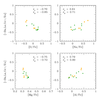
Figure 22: The ratio [$<$Ba,La,Ce$>$/Eu] as a function of the proton capture elements O. Na, Mg, Al for stars with UVES spectra of the MP (green symbols) and MR (orange symbols) component in NGC 1851. Spearman rank correlation coefficient and Pearson linear regression correlation coefficient are indicated in each panel.

6 Comparison of spectroscopy and photometry in NGC 1851

NGC 1851 is clearly a complex globular cluster. Using our unprecedented large dataset of chemical abundances we may hope to have a better tagging of the observed broadening and/or splitting of photometric sequences and to have a deeper insight on their origin.

In Fig. 23 we summarize in six CMDs the results of a first screening of RGB stars in NGC 1851 using the $y$ Strömgren magnitude and the $hk$ index kindly provided by prof. Jae-Woo Lee. In each panel we plot the giants of NGC 1851 in common between the present study and the work of Lee and collaborators (121 stars), colour-coded according to their abundances, larger or lower than the average value for the common sample, listed in each panel of Fig. 23.

Before discussing these plots, we notice that within NGC 1851, $hk$ is extremely well correlated with the Strömgren index $m_{1}$ (see Fig. 24). However, from our result, these indexes do neither appear to trace the metallicity of NGC 1851 stars (panel (a)), nor seem to be well correlated with a difference in [Ca/H], as shown in panel (b). Admittedly, as discussed in Section 4.2, the difference in [Fe/H] between the MR and MP components in NGC 1851 is small and might not be the best indicator to separate stellar components in this peculiar cluster. However, the separation between these components is real, as shown by their different radial distribution (Fig. 1 in Carretta et al. 2010c). Yet, the $hk$ index seems to be blind to this difference.

On the other hand, in monometallic clusters $m_{1}$ measures the strength of the near-UV CN bands, and it is strongly correlated with N abundances in metal-rich clusters (see Carretta et al. 2011). It may well be used to separate first and second generation stars in NGC 1851 (see Fig. 25). So, it is not surprising that also $hk$ seems to be quite efficient in separating first and second generation stars in NGC 1851, judging from panel (c) in Fig. 23. In this panel we did not adopt the average value for [Na/Fe] (+0.189 dex for stars in common between us and Lee et al.), but we chose the value 0.0 that in NGC 1851 divides first and second generation stars according to the definition in Carretta et al. (2009a). The two stellar generations are separated very well in the $y-hk$ plane. The same result would hold also using the ratio [O/Na], although the separation is not so clean as in panel (c) due to the presence of upper limits and/or larger errors in the O abundances.

The efficiency of $hk$ to separate first and second generation stars is also supported by the CMDs in panels (d) and (e). Of course, separation of first and second generation stars using Mg and Si is less accurate, because the spread in abundances is not very large. However, the striking evidence in these two panels is that the two groups are specularly selected, as expected due to the anticorrelation of Mg and Si.

The final panel (f) shows how stars are segregated along the split red giant branch in NGC 1851 according to their Ba abundances. In this plane (but also in the Strömgren $v,v-y$ CMD, where the split is even clearer) only Ba-rich stars are found on the reddest section of the RGB, whereas Ba-poor stars are mostly (but not exclusively) restricted to the bluest side of the RGB. This finding confirms and strengthens a similar result by V10, based on a much more limited sample. At a given level of magnitude, all stars having high values of the $hk$ index are more Ba-strong than the average [Ba/Fe] value, although there is not a one-to-one correspondence between Ba and $hk$.

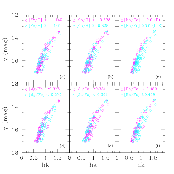
Figure 23: RGB stars in common between our analysis and that by Lee et al. (2009a) in the $y$-$hk$ plane from Strömgren photometry. In each panel stars are color coded according to their abundances derived in the present study. The elements and the separating values are indicated in each panel.

Summarizing the results of this Section, we found that in NGC 1851 the $hk$ index seems to be related to the dichotomy first/second generation, but not to the Ca abundance: in Fig. 26 we also show the direct correspondence between $hk$ and our [Ca/H] values from spectroscopy, and we do not see any correlation.

In Carretta et al. (2009b) we demonstrated that in CMDs including the $u$ band, second generation stars which are N-enhanced, as expected from the full action of the complete CNO-cycle, are spread out to the red, along the RGB. The link between chemical composition and observed colours in first and second generation stars is examined in detail in another paper (Carretta et al. 2011), but from Fig. 11 and Fig. 23 we can conclude tentatively that $hk$ separates stars that are N-rich and N-poor, respectively. We notice that this result is unexpected, given the definition of the Ca narrow band of Lee et al. (2009).

Figure 24: Plot of $m_{1}$ and $hk$ for stars in NGC 1851 in common between our work and Lee et al. (2009a). Stars with higher values for $m_{1}$ and $hk$ are the brighter ones of the sample.

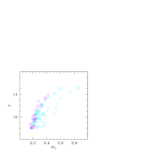
Figure 25: Plot of $m_{1}$ vs $y$ for stars in NGC 1851, separated in first (P, in magenta) and second (IE, in light blue) stars.

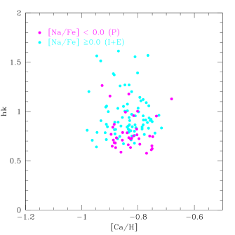
Figure 26: $hk$ index by Lee and collaborators as a function of the [Ca/H] ratio derived in the present study for giants in NGC 1851.

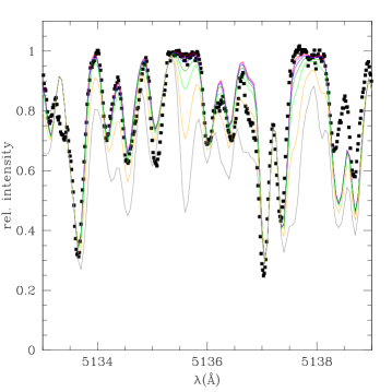
Figure 27: Portion of the UVES spectrum of star 32903 in the C₂ region at 5135 Å (filled squares) with synthetic spectra computed for various C abundances ([C/Fe]=-0.5,-0.4,-0.3,-0.2,-0.1,0.0,+0.1).

6.1 The effect of (neglecting) carbon

Judging from panel (c) and (f) of Fig. 23, there is a global correspondence between Ba-rich and N-rich stars, but there are exceptions. This is a significant difference with respect to the very tight sequences shown by V10 with their limited sample, and it suggests that this is not the whole story.

Another possible player to be considered might be the carbon abundance. In another paper (Carretta et al. 2011) we studied in detail the effect of variations of N and C abundances on the Strömgren photometry. Here we only summarize in Fig. 28 the main results relative to the C abundance variations. Briefly, we used a model atmosphere with the parameters T${}_{\rm eff}=4478$ K, $\log g=1.4$ and [A/H]=-1.23 and we computed two synthetic spectra for a C-rich, N-rich and a C-rich, N-poor case, respectively. Afterwards, we evaluated the differences in magnitude with respect to the reference case of a C-normal, N-poor star and we plot in the left and right panels of Fig. 28 the displacements due to variation in only N (red line) and also in C (blue line).

From this exercise it is easy to see that for N-poor stars, the impact of varying C is modest. The main reason is that in these stars O $>$ C, and then CN bands are not very strong. On the other hand, for N-rich stars there is a notable effect when changing the C abundance, in particular in the $v$ filter. In turn, this implies large variations in indices like $c_{1}$ and $m_{1}$.

From these computations and from the CMDs in Fig. 28 we could think that stars on the redder sequence of NGC 1851 are quite good candidate to be C-rich and N-rich (hence O-poor). On the other hand, the C-rich and N-poor stars (i.e. O-rich) may not be separated from the other N-poor, C-normal stars in none of the Strömgren indices. This might well explain the fact that the reddest RGB sequence is only made by a trickling string of few stars: they might be not all the C-rich stars present in the cluster, but only those that are also O-poor. In general, it is likely that the C-rich stars in NGC 1851 would coincide with the Ba-rich stars, and might correspond to our definition of MR population (Sect. 4.2), related to the brighter SGB and to the red HB according to their number ratios.

However, the evidence supporting this view is currently limited to the Strömgren photometry. We did not find evidence of C₂ in our spectra, even for the most Ba-rich (and also metal-rich) stars with UVES spectra (stars 32903 and 41689: see Fig. 27). In the first case, we can even set a quite stringent upper limit of [C/Fe]$<-0.4$, incompatible with the assumption of C $\sim$ O which is basic in the scenario discussed in this section. Of course, it is possible that C has been transformed into N in these very bright giants, and that CN bands are very strong, due to a very large excess of N. Unluckily, we could not prove this with the present spectroscopic data.

7 Discussion and conclusions

There are several observations in NGC 1851 suggesting that two (originally) distinct objects may have concurred to form the currently observed cluster: the bimodal distribution of the HB, the double/split SGB, and the splitting recently found on the RGB. To this, in Carretta et al. (2010c) we added a distinct radial distribution, with the MP component more centrally concentrated. When coupled with the existence of the Na-O anticorrelation in each component on the RGB, although with different primordial/polluted ratios of stars, this series of evidence points toward the existence of two merged clusters. The results from the previous Section fit reasonably well a scenario where the two clusters differ also for the average level of Ba (and probably also C) abundance, with however additional complications that will be commented in the next subsection.

Our idea offers the advantage of accounting for a number of observations with the minimum of assumptions. For most aspects, these essentially reduce to only one, that of an age difference of about 1 Gyr between the two putative clusters (since the metallicity difference - the other necessary assumption - is actually measured from our data). The age difference stems in part because we can exclude a significant contribution from He variations: the moderate extensions of both the Na-O and Al-Mg anticorrelations indicate that they must be not relevant. This minor role of He variations is moreover confirmed by the constant luminosity level between the red and the blue HB (see Cassisi et al. 2008). An age difference of $\sim 1$ Gyr is also compatible with the higher level in $s-$process elements found for the MR component.

Figure 28: Strömgren $v,v-y$ and $v,m_{1}$ for the MP and MR components in NGC 1851. In both panels the red and blue lines indicate the effect of a N and a C variation, respectively, on the stars’ colours (see text).

The combination of age and metallicity differences implies a difference of only 0.04 $M_{\odot}$ in the masses of stars currently on the RGB, which is compatible with the HB but results into a negligible segregation of the two populations in the region of the cluster we observed. A primordial segregation between the MP and MR populations might then have survived the following dynamical evolution.

Finally, there might also be a difference in the C content between the two putative GCs; this is not only expected if the MR one is about 1 Gyr younger (allowing the contribution of AGB stars with masses $<3\leavevmode\nobreak\ M_{\odot}$), but could also possibly account for the observed Strömgren colours. However, we did not detect any C₂ line in our spectra, which possibly contradicts the hypothesis of a significant C enhancement (unless this is cancelled by evolutionary effects).

In summary, most observations concerning NGC 1851 can be explained by the existence of two sub-populations:

A first one, including about 35-40% of the stars, that behaves like a small globular cluster, with a normal Na-O anticorrelations and normal features. The only peculiar characteristic is maybe a number of primordial stars higher than the average $\sim 30\%$ typical of GCs. This first population may be linked to the faint SGB (Milone et al. 2008) and to the BHB and is more centrally concentrated in NGC 1851, according to our RGB sample.

A second population, formed by the remaining 60-65% of stars, that is represented by our MR component, more rich in Ba and $s-$process elements, stronger, on average, in their $hk$ index, and with a behaviour in the Strömgren photometric indices well explained by an overabundance of C. This population, that is possible to identify with the bright SGB and the RHB, is not very different in [Fe/H] or [Ca/H] from the first one, although it is clearly more enriched in these elements. The most significant difference, however, seems to concern the products from the third dredge-up, which implies an age difference large enough to allow low mass stars to contribute. We also note that even if the content of C of the MR population is perhaps higher than that in the MP population, the C+N+O sum is probably not very different (0.1-0.2 dex, all concentrated on the C term), because C $\ll$ (N+O) anyway. The contribution of low mass ($\sim 2-3M_{\odot}$) stars is also required by the heavy-to-light ratio for the $s-$process elements.

7.1 The correlation between proton and neutron capture elements

We confirm and extend the results found by Yong and Grundahl (2008): in NGC 1851 the abundances of $s-$process dominated elements seems to be strictly related to those of the light elements involved in $p-$capture reactions. The level of neutron capture elements increases for stars where the signature of processing by H-burning at high temperature is more marked. While this signature is very clean within the MR population, its presence is not obvious on the MP one, depending on the membership of a couple of stars.

This observation bears a potential problem, depending on the mechanism assumed for the origin of the $s-$process elements (e.g. Käppeler 1999). If, as also suggested by the high heavy-to-light ratio, they were forged by the main component (e.g. by low mass stars with $M_{ZAMS}\sim 1.5-3M_{\odot}$ during the AGB phase), then the evolutionary times of these stars are ranging from about 340 Myr up to about 2 Gyr (e.g. Schaller et al. 1992). However, if AGB stars with 4-8 $M_{\odot}$ are responsible for the $p-$capture elements, the release of polluted matter from these stars is expected as soon as about 40 Myr and as late as 160 Myr (the timescale for the production of $p-$capture elements would be even shorter were they produced by massive stars). This timescale problem could be bypassed only if the gas cumulates in a reservoir which does not form stars for several 10⁸ yrs.

Such a time delay can perhaps be accommodated in models with a cooling flow as tentatively proposed by D’Ercole et al. (2008) if e.g. a threshold in the mass of gathering gas is necessary to trigger the formation of the second generation. In addition, whether the correlation between $n-$ and $p-$capture elements were continuous, dilution of the material of this reservoir with unprocessed material would be required. Unluckily, our data are not accurate enough to favour or dismiss this last hypothesis.

An alternative possibility would be that the same stars produced both $n-$ and $p-$capture elements, as recently suggested by D’Antona et al. (2011) to explain a similar problem for $\omega$ Cen. Such an hypothesis meets several difficulties, for instance the lack of correlation between $n-$ and $p-$capture elements in most GCs. Furthermore, the only known mechanism producing the $n-$capture elements in massive stars (the weak component: Raiteri et al. 1991) is a secondary mechanism (then likely negligible in metal-poor stars) which preferentially produces the less massive among elements along the $s-$chain, and e.g. likely a significant fraction of Cu. At variance with the recent case of M 22 (Marino et al. 2011), we do not find any sign of Cu production within NGC 1851, and the heavy-to-light ratio is large.

It then seems that the correlations between $p-$ and $n-$capture elements in NGC 1851 observed by us and Yong and Grundahl (2008) put serious constraints to the scenario of pollution in GCs from AGB stars.

7.2 Hunting for the ancestral galaxy

The idea proposed by van den Bergh (1996), that GCs with a composite CMD are the result of a merger of two parent clusters within the past equivalent of a present-day dwarf spheroidal, offers several attractive hints to explain the peculiarities observed in NGC 1851.

First, the N-body simulations by Makino et al. (1991) show that orbital angular momentum is transferred at earlier stages to the escaping particles: this process favours the shrinkage of the orbit, hence the merger. Nowadays, we are aware that a large loss of stars is expected at early phases from a proto-GC, since this is required by the observed composition of first and second generation stars (see e.g. Carretta et al. 2010a; Conroy 2011). Should the early cluster evolution occurs in the environment of a dSph, this large mass loss may actually help the merger process.

If the clusters were in the same dwarf galaxy, they might have both spiralled to the centre (by dynamical friction) and then merged in the currently observed object. A necessary condition for this chain of events is that the dSph must have survived at least for a few Gyr to the interaction with our Galaxy. Cases for dSphs hosting a system of GCs of their own are well known (Fornax, and the disrupting Sagittarius dwarf).

On the other hand, the different density distribution of MP and MR stars suggests that the merging of the two clusters occurred not too long in the past, less than a few Gyr ago. Since this merging should have happened before the putative dwarf spheroidal dissolved, it is possible that the remains of this ancestral, parent galaxy can still be traced around NGC 1851. Recently, a study by Olszewski et al. (2009) found that the cluster is embedded in a halo 500 pc across, corresponding to about 0.1% of the dynamical mass of NGC 1851. The two populations - as represented by twin MSs and SGBs - are traced up to more than 2.85 tidal radii from the cluster centre, incidentally contradicting the finding by Zoccali et al. (2009) on a strong radial gradient for the SGB. More recently, Carballo-Bello & Martinez-Delgado (2010) detected with the ESO-WFI a clearly traceable MS of extra-tidal stars around NGC 1851 and NGC 1904. It is interesting to note that both studies do not find evidence for collimated structure and both conclude against the evidence of tidal tails: NGC 1851 is simply embedded in a smooth, giant cloud of tidal debris.

According to Carballo-Bello & Martinez-Delgado, it is tempting to associate this overdensity to the debated Canis Major dwarf system: this conclusion would be corroborated by the observation that the old and metal-poor population of the debris cover a sky-projected distance of about 3.3 kpc, similar to the distance between NGC 1851 and NGC 1904. Both clusters are considered (with NGC 2298 and NGC 2808) to be part of the Canis Major system (Martin et al. 2004). On the other hand, Olszewski et al. (2009) conclude that from existing dynamical models it is not possible to discriminate between isolated cluster evaporation and destruction of a dwarf galaxy, for the origin of the observed giant halo around NGC 1851.

Is this cluster an exception? NGC 1851 shares several characteristics with another, more metal-poor cluster: M 22. Marino et al. (2009, 2011) found two sub-populations differing both in Fe and Ba, in this cluster, with the abundance of $s-$process elements correlated with the iron abundance. The metallicity spread they found (0.10 dex $r.m.s.$ scatter) is not much different from the values found by high resolution spectra by us (0.07 dex) or by Yong and Grundahl (2008; 0.084 dex) for NGC 1851, and the metal-rich population is also Ca-rich with respect to the metal-poor one.

Finally, we also note that the merger hypothesis was recently considered by Lane et al. (2010a) to account for some kinematic features not well explained for the globular cluster 47 Tuc. For example, Lane et al. (2010b) note that a merger between two clusters with similar metallicity “would have increased the total luminosity of 47 Tuc without altering its $M/L_{V}$ significantly”: this results in the cluster being an outlier in their $M/L_{V}$ vs $M_{V}$ relation. However, a two component model with populations having two distinct kinematics is favoured in the case of 47 Tuc, whereas no significant kinematic difference can be established between the two populations in NGC 1851, apart from the observed radial segregation of stars on the RGB.

It is thus just possible that several channels are viable for the formation of different “flavours” of globular clusters. Beside the large, massive GCs spiralling in the nucleus of their own galaxy, finding only a nuclear diffuse component, as is the case of M 54 and perhaps $\omega$ Cen (e.g. Carretta et al. 2010b), possibly another channel is feasible: the merger of two GCs in the same parent galaxy before the disruption within a much larger galaxy.

However, more observations are needed to settle the case of NGC 1851. In the future, we plan to analyse CN and CH low resolution spectra of SGB stars in each of the two SGBs found in NGC 1851 to investigate the role of C and N abundances. We also intend to test our hypothesis of a cluster merger by exploring the Na-O anticorrelation in both the BHB and RHB of this intriguing cluster.

Appendix A Error estimates

We refer the reader to the analogous Appendices in Carretta et al. (2009a,b) for a detailed discussion of the procedure adopted for error estimates. In the following we only provide the main tables of sensitivities of abundance ratios to the adopted errors in the atmospheric parameters and $EW$s and the final estimates of internal and systematic errors for all species analysed from UVES and GIRAFFE spectra of stars in NGC 1851.

The sensitivities of derived abundances on the adopted atmospheric parameters were obtained by repeating our abundance analysis by changing only one atmospheric parameter each time for $all$ stars in NGC 1851 and taking the average value of the slope change vs. abundance. This exercise was done separately for both UVES and GIRAFFE spectra.

We notice that when estimating the contribution to internal errors due to EWs and $v_{t}$, the values usually adopted (determined from the scatter of abundances from individual lines) are overestimated, because regularities in the data are not taken into account. These regularities are due to uncertainties in the $gf-$values, unrecognised blends with adjacent lines, not appropriate positioning of the continuum, etc. They show up in uniform deviations of individual lines from average abundances for each star. By averaging over all stars the residuals of abundances derived from individual lines with respect to the average value for each star, we estimated that some 36% of the total variance in the Fe abundances from individual lines is due to systematic offsets between different lines, which repeat from star-to-star. For about 30% of the line, these offsets have trends with temperature significant at about 2 $\sigma$ level. However, we found that the additional fraction of variance that can be explained by these trends is very small, and we can neglect it. We conclude that when considering star-to-star variations (internal errors, according to our denomination), the errors in EWs and $v_{t}$ should be multiplied by 0.8.

The amount of the variations in the atmospheric parameters is shown in the first line of the headers in Table 14, and Table 15, whereas the resulting response in abundance changes of all elements (the sensitivities) are shown in columns from 3 to 6 of these tables.

Table 14: Sensitivities of abundance ratios to variations in the atmospheric parameters and to errors in the equivalent widths, and errors in abundances for stars in NGC 1851 observed with UVES

Element	Average	Teff	$\log g$	[A/H]	$v_{t}$	EWs	Total	Total
	n. lines	(K)	(dex)	(dex)	kms-1	(dex)	Internal	Systematic
Variation		50	0.20	0.10	0.10
Internal		4	0.04	0.06	0.04	0.070
Systematic		36	0.06	0.03	0.01
$[$Fe/H$]$i	82	+0.039	+0.024	+0.006	$-$0.034	+0.008	0.017	0.033
$[$Fe/H$]$ii	9	$-$0.063	+0.107	+0.036	$-$0.015	+0.023	0.039	0.064
$[$O/Fe$]$i	2	$-$0.019	+0.060	+0.028	+0.034	+0.048	0.054	0.071
$[$Na/Fe$]$i	4	+0.017	$-$0.056	$-$0.039	+0.016	+0.034	0.043	0.074
$[$Mg/Fe$]$i	3	$-$0.007	$-$0.017	$-$0.008	+0.019	+0.039	0.040	0.011
$[$Al/Fe$]$i	2	+0.012	$-$0.029	$-$0.014	+0.031	+0.048	0.051	0.066
$[$Si/Fe$]$i	9	$-$0.055	+0.021	+0.008	+0.025	+0.023	0.026	0.043
$[$Ca/Fe$]$i	17	+0.037	$-$0.037	$-$0.020	$-$0.022	+0.016	0.023	0.030
$[$Sc/Fe$]$ii	8	+0.053	$-$0.028	$-$0.006	$-$0.019	+0.024	0.026	0.045
$[$Ti/Fe$]$i	9	+0.058	$-$0.030	+0.008	$-$0.003	+0.023	0.024	0.047
$[$Ti/Fe$]$ii	1	+0.042	$-$0.021	$-$0.003	+0.009	+0.068	0.068	0.034
$[$V/Fe$]$i	8	+0.072	$-$0.018	$-$0.003	+0.007	+0.024	0.025	0.057
$[$Cr/Fe$]$i	3	+0.029	$-$0.025	$-$0.017	+0.018	+0.039	0.041	0.026
$[$Cr/Fe$]$ii	12	+0.019	$-$0.030	$-$0.018	+0.003	+0.020	0.023	0.031
$[$Mn/Fe$]$i	3	+0.021	$-$0.015	$-$0.009	$-$0.001	+0.039	0.040	0.025
$[$Co/Fe$]$i	5	$-$0.009	+0.002	+0.002	+0.024	+0.030	0.032	0.017
$[$Ni/Fe$]$i	29	$-$0.018	+0.017	+0.007	+0.015	+0.013	0.015	0.017
$[$Cu/Fe$]$i	1	+0.011	$-$0.074	+0.044	$-$0.084	+0.068	0.081	0.032
$[$Y/Fe$]$ii	5	+0.041	$-$0.007	+0.008	$-$0.085	+0.030	0.046	0.052
$[$Zr/Fe$]$i	4	+0.087	$-$0.020	$-$0.018	+0.027	+0.034	0.038	0.074
$[$Zr/Fe$]$ii	1	+0.092	$-$0.099	$-$0.036	$-$0.087	+0.068	0.082	0.079
$[$Ba/Fe$]$ii	4	+0.083	$-$0.050	+0.004	$-$0.120	+0.034	0.060	0.096
$[$La/Fe$]$ii	2	+0.110	$-$0.180	$-$0.036	$-$0.035	+0.048	0.066	0.106
$[$Ce/Fe$]$ii	1	+0.063	$-$0.027	$-$0.007	$-$0.005	+0.068	0.069	0.072
$[$Nd/Fe$]$ii	2	+0.073	$-$0.043	$-$0.011	$-$0.105	+0.048	0.065	0.069
$[$Eu/Fe$]$ii	2	+0.110	$-$0.087	+0.014	+0.010	+0.048	0.053	0.089
$[$Dy/Fe$]$ii	1	+0.078	$-$0.026	$-$0.002	$-$0.005	+0.068	0.069	0.066

Table 15: Sensitivities of abundance ratios to variations in the atmospheric parameters and to errors in the equivalent widths, and errors in abundances for stars in NGC 1851 observed with GIRAFFE

Element	Average	Teff	$\log g$	[A/H]	$v_{t}$	EWs	Total	Total
	n. lines	(K)	(dex)	(dex)	kms-1	(dex)	Internal	Systematic
Variation		50	0.20	0.10	0.10
Internal		4	0.04	0.03	0.14	0.111
Systematic		51	0.06	0.06	0.02
$[$Fe/H$]$i	31	+0.056	$-$0.006	$-$0.002	$-$0.035	+0.020	0.043	0.057
$[$Fe/H$]$ii	3	$-$0.032	+0.091	+0.024	$-$0.012	+0.064	0.057	0.043
$[$O/Fe$]$i	1	$-$0.045	+0.090	+0.033	+0.036	+0.111	0.100	0.059
$[$Na/Fe$]$i	3	$-$0.013	$-$0.029	$-$0.013	+0.023	+0.064	0.058	0.035
$[$Mg/Fe$]$i	2	$-$0.022	$-$0.003	$-$0.004	+0.021	+0.078	0.067	0.023
$[$Si/Fe$]$i	7	$-$0.053	+0.034	+0.009	+0.029	+0.042	0.048	0.055
$[$Ca/Fe$]$i	5	+0.003	$-$0.030	$-$0.005	$-$0.002	+0.050	0.040	0.010
$[$Sc/Fe$]$ii	5	$-$0.058	+0.087	+0.029	+0.013	+0.050	0.047	0.065
$[$Ti/Fe$]$i	4	+0.020	$-$0.004	$-$0.010	+0.015	+0.056	0.048	0.021
$[$V/Fe$]$i	6	+0.030	$-$0.001	$-$0.010	+0.020	+0.045	0.043	0.033
$[$Cr/Fe$]$i	4	+0.003	$-$0.002	$-$0.008	+0.026	+0.056	0.053	0.012
$[$Co/Fe$]$i	1	+0.004	+0.019	+0.005	+0.025	+0.111	0.093	0.014
$[$Ni/Fe$]$i	7	$-$0.015	+0.024	+0.005	+0.018	+0.042	0.040	0.018
$[$Zr/Fe$]$i	2	+0.066	$-$0.013	$-$0.014	+0.031	+0.078	0.072	0.086
$[$Ba/Fe$]$ii	1	$-$0.043	+0.041	+0.044	$-$0.030	+0.111	0.097	0.051