Confronting Intractability via Parameters

Happy 60th Birthday Mike!

Abstract

One approach to confronting computational hardness is to try to understand the contribution of various parameters to the running time of algorithms and the complexity of computational tasks. Almost no computational tasks in real life are specified by their size alone. It is not hard to imagine that some parameters contribute more intractability than others and it seems reasonable to develop a theory of computational complexity which seeks to exploit this fact. Such a theory should be able to address the needs of practicioners in algorithmics. The last twenty years have seen the development of such a theory. This theory has a large number of successes in terms of a rich collection of algorithmic techniques both practical and theoretical, and a fine-grained intractability theory. Whilst the theory has been widely used in a number of areas of applications including computational biology, linguistics, VLSI design, learning theory and many others, knowledge of the area is highly varied. We hope that this article will show both the basic theory and point at the wide array of techniques available. Naturally the treatment is condensed, and the reader who wants more should go to the texts of Downey and Fellows [125], Flum and Grohe [155], Niedermeier [240], and the upcoming undergraduate text Downey and Fellows [127].

1 Introduction

1.1 Preamble

There is little question that the computer has caused a profound change in society. At our fingertips are devices that are performing billions of computations a second, and the same is true of embedded devices in all manner of things. In the same way that much of mathematics was developed to understand the physics of the world around us, developing mathematics to understand computation is an imperative. It is little wonder that the famous ${\sf P}^{\mbox{?}\atop\mbox{${}_{\mbox{=}}$}}{\sf NP}$ question is one of the Clay Prize questions and is regarded by some as the single most important problem in mathematics. This question is one in complexity theory which seeks to understand the resources (such as time or space) needed for computation.

The goal of this paper is to describe the methods and development of an area of complexity theory called parameterized complexity. This is a fine-grained complexity analysis which is often more attuned to analyzing computational questions which arise in practice than traditional worst case analysis. The idea here is that if you are working in some computational science and wish to understand what is feasible in your area, then perhaps this is the methodology you should know.

As articulated by the first author in [116], people working in the area tend to be a bit schizophrenic in that, even in computer science, paper reviews range from saying that “parameterized complexity is now well known so why are you including this introductory stuff?”, to the other extreme where reviewers say that they have never heard about it.

Whilst the use of parameterized complexity in applications has been growing at a very fast rate, there still remain significant groups who seem unaware of the techniques and ideas of the area. Everyone, apparently, is aware of NP-completeness and seems vaguely aware of randomized or approximation techniques. However, this seems not to be the case yet for parameterized complexity and/or algorithms. Moreover, it is certainly not the case that parameterized complexity has become part of the standard curriculum of theoretical computer science as something all researchers in complexity should know.

1.2 The issue

In the first book on the subject by Downey and Fellows [125], much is made of the issue “what is the role of complexity theory?”. After the work of Alan Turing and others in the mid-20th century, we understand what it means for something to be computable. But for actual computations, it is not enough to know that the problem is computable in theory. If we need to compute something it is not good if the running time will be so large that no computer ever conceived will be able to run the computation in the life time of the universe. Hence, the goal is to understand what is feasible. The point is that for any combinatorial problem, we will deal with only a small finite fraction of the universe, so how do we quantify this notion of feasibility? Classically, this is achieved by identifying feasibility with polynomial-time computability.

When we first learn of this, many of us immediately think of polynomial like $n^{10^{5000}}$ and say “surely that is not feasible!”. We tend to forget that, because of such intuitive objections, the original suggestions that asymptotic analysis was a reasonable way to measure complexity and polynomial time was a reasonable measure of feasibility, were initially quite controversial. The reasons that the now central ideas of asymptotic polynomial time (P-time) and NP-completeness have survived the test of time are basically two. Firstly, the methodologies associated with polynomial-time and P-time reductions have proved to be readily amenable to mathematical analysis in most situations. In a word, P has good closure properties. It offers a readily negotiable mathematical currency. Secondly, and even more importantly, the ideas seem to work in practice: for “natural” problems the universe seems kind in the sense that (at least historically) if a “natural” computational problem is in P then usually we can find an algorithm having a polynomial running time with small degree and small constants. This last point, while seeming a religious, rather than a mathematical, statement, seems the key driving force behind the universal use of P as a classification tool for “natural” problems.

Even granting this, the use of things like NP-completeness is a very coarse tool. We are given some problem and show that it is NP-complete. What to do? As pointed out in Garey and Johnson [172], this is only an initial foray. All such a result says is that our hope for an exact algorithm for the general problem which is feasible is likely in vain.

The problem with the standard approach of showing NP-completeness is that it offers no methodology of seeking practical and feasible algorithms for more restricted versions of the problem which might be both relevant and feasible. As we will see, parameterized complexity seeks to have a conversation with the problem which enables us to do just that.

1.3 The idea

The idea behind parameterized complexity is that we should look more deeply into the actual structure of the problem in order to seek some kind of hidden feasibility. Classical complexity views a problem as an instance and a question. The running time is specified by the input’s size.

Question : When will the input of a problem coming from “real life” have no more structure than its size?

Answer : Never!

For real-world computations we always know more about the problem. The problem is planar, the problem has small width, the problem only concerns small values of the parameters. Cities are regular, objects people construct tend to be built in some comprehensible way from smaller ones constructed earlier, people’s minds do not tend to work with more than a few alternations of quantifiers, etc. Thus, why not have a complexity theory which exploits these structural parameters? Why not have a complexity theory more fine-tuned to actual applications?

1.4 The contribution of this article

Before we launch into examples and definitions, we make some remarks about what this article offers. The area of parameterized complexity (as an explicit discipline) has been around for around 20 years. The group or researchers who have adopted the methodology most strongly are those (particularly in Europe) who are working in applications. What has emerged is a very rich collection of distinctive positive techniques which should be known to researchers in computational applications in areas as diverse as linguistics, biology, cognition, physics, etc. The point here is that once you focus on a an extended “computational dialog” with the problem new techniques emerge around this. These techniques vary from simple (and practical) local reduction rules (for example Karsten Weihe’s solution to the “Europe train station problem” [280]) to some which are highly theoretical and use some very deep mathematics (for example, the recent proof that topological embedding is fixed-parameter tractable by Grohe, Kawarabayashi, Marx, and Wollan [180], which uses most of the structure theory of the Graph Minors project of Robertson and Seymour [253]).

The second part of this article looks at these positive techniques systematically, and we hope that the reader will find useful tools there. This area is still rapidly developing, and there are many internal contests amongst the researchers to develop techniques to beat existing bounds. For further details, the reader can see the web site http://fpt.wikidot.com/ .

The first part of the article is devoted to limitations. It is worth mentioning that the area is concerned with tractability within polynomial time. Hence classical methods do not readily apply. The question is “how does the problem resides in polynomial time”. To illustrate this, we begin with the basic motivating examples.

Vertex Cover
Instance:  A graph $G=(V,E)$.
Parameter: A positive integer $k$.
Question:  Does $G$ have a vertex cover of size $\leq k$? (A vertex cover of a graph $G$ is a set $S\subseteq V(G)$ such that for all edges $\{x,y\}$ of $G$, either $x\in S$ or $y\in S$.)

Dominating Set
Instance: A graph $G$.
Parameter: A positive integer $k$.
Question: Does $G$ have a dominating set of size $k$? (A dominating set is a set $S\subseteq V(G)$ where, for each $u\in V(G)-S$ there is a $v\in S$ such that $\{u,v\}\in E(G)$.)

Of course both of these problems (without the parameter) are famously NP-complete by the work of Karp [201]. With the parameter fixed then both of the problems are in polynomial time simply by trying all of the ${n}\choose{k}$ subsets of size $k$ where $n$ is the number of vertices of the input graph $G$. What we now know is that there is an algorithm running in time $1.2738^{k}+O(n)$ (see [68]) (i.e., linear time for a fixed $k$ and with an additive component that is mildly exponential in $k$), whereas the only known algorithm for Dominating Set is to try all possibilities. This takes time more or less $n^{k}$. Moreover, we remark that the methods for solving Vertex Cover are simple reduction rules which are “industrial strength” in that they run extremely well in practice (e.g. [60, 216]), even for $k$ beyond which would seem reasonable, like $k=2000$. The reader might wonder: does this matter? Table 1 from the original book [125] illustrates the difference between a running time of $\Omega(n^{k+1})$ (that is, where exaustive search is necessary) and a running time of $2^{k}n$. The latter has been achieved for several natural parameterized problems. (In fact, as we have seen above, the constant $2^{k}$ can sometimes be significantly improved and its contribution can sometimes even be additive.)

	$n=50$	$n=100$	$n=150$
$k=2$	625	2,500	5,625
$k=3$	15,625	125,000	421,875
$k=5$	390,625	6,250,000	31,640,625
$k=10$	$1.9\times 10^{12}$	$9.8\times 10^{14}$	$3.7\times 10^{16}$
$k=20$	$1.8\times 10^{26}$	$9.5\times 10^{31}$	$2.1\times 10^{35}$

Table 1: The Ratio $\frac{n^{k+1}}{2^{k}n}$ for Various Values of $n$ and $k$.

Even before we give the formal definitions, the intent of the definitions will be clear. If we have algorithms running in time $n^{c}$, for some $c$ that is independent of $k$, we regard this as being (fixed-parameter) tractable, and if $c$ increases with $k$, then this problem is regarded as being intractable. In the latter case, we cannot usually prove intractability as it would separate P from NP, as it would in the case of Dominating Set, for example. But we can have a completeness programme in the same spirit as NP-completeness.

We mention that the methodology has deep connections with classical complexity. For example, one of the more useful assumptions for establishing lower bounds in classical complexity is what is called the exponential time hypothesis (ETH) which is that not only is $n$-variable 3SAT not in polynomial time, but in fact it does not have an algorithm running in subexponential time. (Impagliazzo, Paturi and Zane [196]). With this hypothesis, many lower bounds can be made rather sharp. Recently Chen and Grohe demonstrated an isomorphism between subexponential time complexity and parameterized complexity [76]. The connection between subexponential time complexity and parameterized complexity was noticed long ago by Abrahamson, Downey and Fellows [2]. Another notable connection is with polynomial time approximation schemes. Here the idea is to give a solution which is approximate to within $\epsilon$ of the correct solution. Often the PCP theorem allows us to show that no such approximation scheme exists unless P$=$NP. But sometimes they do, but can have awful running times. For example, here is a table from Downey [116]:

• Arora [22] gave a $O(n^{\frac{3000}{\epsilon}})$ PTAS for Euclidean Tsp

• Chekuri and Khanna [61] gave a $O(n^{12(\log({1/\epsilon})/\epsilon^{8})})$ PTAS for Multiple Knapsack

• Shamir and Tsur [266] gave a $O(n^{2^{2^{\frac{1}{\epsilon}}}-1)})$ PTAS for Maximum Subforest

• Chen and Miranda [73] gave a $O(n^{(3mm!)^{\frac{m}{\epsilon}+1}})$ PTAS for General Multiprocessor Job Scheduling

• Erlebach et al. [138] gave a $O(n^{\frac{4}{\pi}(\frac{1}{\epsilon^{2}}+1)^{2}(\frac{1}{\epsilon^{2}}+2)^{2}})$ PTAS for Maximum Independent Set for geometric graphs.

Table 2 below calculates some running times for these PTAS’s with a 20% error.

Reference	Running Time for a 20% Error
Arora [22]	$O(n^{15000})$
Chekuri and Khanna [61]	$O(n^{9,375,000})$
Shamir and Tsur [266]	$O(n^{958,267,391})$
Chen and Miranda [73]	$>O(n^{10^{60}})$
	(4 Processors)
Erlebach et al. [138]	$O(n^{523,804})$

Table 2: The Running Times for Some Recent PTAS’s with 20% Error.

Downey [116] argues as follows:

“By anyone’s measure, a running time of $n^{500,000}$ is bad and $n^{9,000,000}$ is even worse. The optimist would argue that these examples are important in that they prove that PTAS’s exist, and are but a first foray. The optimist would also argue that with more effort and better combinatorics, we will be able to come up with some $n\log n$ PTAS for the problems. For example, Arora [23] also came up with another PTAS for Euclidean Tsp, but this time it was nearly linear and practical.

But this situation is akin to P vs NP. Why not argue that some exponential algorithm is just the first one and with more effort and better combinatorics we will find a feasible algorithm for Satisfiability? What if a lot of effort is spent in trying to find a practical PTAS’s without success? As with P vs NP, what is desired is either an efficient PTAS (EPTAS), or a proof that no such PTAS exists. A primary use of NP-completeness is to give compelling evidence that many problems are unlikely to have better than exponential algorithms generated by complete search.”

The methods of parameterized complexity allow us to address the issue. Clearly, the bad running times are caused by the presence of $\frac{1}{\epsilon}$ in the exponent. What we could do is parameterize the problem by taking the parameter to be $k=\frac{1}{\epsilon}$ and then perform a reduction to a kind of core problem (see Subsection 3.5). If we can do this, then not only the particular algorithm is infeasible, but moreover, there cannot be a feasible algorithm unless something unlikely (like a miniature P$=$NP) occurs.

1.5 Other coping strategies

Finally, before we move to formal definitions, we mention other strategies which attempt to understand what is feasible. One that springs to mind is the theory of average-case complexity. This has not really been widely applied as the distributions seem rather difficult to apply. Similar comments apply to the theory of smoothed analysis.

In fact one of the reasons that parameterized complexity has been used so often in practice is that it is widely applicable. We also mention that often it can be used to explain unexpected tractability of algorithms. Sometimes they seem to work because of underlying hidden parameters in the input. For example, the number of “lets” in some structured programming languages in practice is usually bounded by some constant, and sometimes engineering considerations make sure that, for example, the number of wafers in VLSI design is small. It is even conceivable there might be a parametric explanation of the tractability of the Simplex Algorithm.

If the reader finds this all useful, then we refer him/her to two recent issues of the The Computer Journal [128] devoted to aspects and applications of parameterized complexity, to the survey of Downey and McCartin [134] on parameterized algorithms, the (somewhat dated) survey Downey [116] for issues in complexity, and other articles such as [131, 132, 142, 141, 143, 126] as well as the books by Downey and Fellows [125], Niedermeier [240] and Flum and Grohe [154].

1.6 Organization and notation

The paper is organized as follows:

In Section 2 we will give the basic definitions and some examples to show the kinds of parameterizations we can look at. We consider as fortunate the fact that a problem can have different parameterizations with different complexities.

In Section 3, we will introduce some of the basic hardness classes, and in particular the main standard of hardness, the class $W[1]$. The gold standard is established by an analog of the Cook-Levin Theorem discussed in Subsection 3.2. Parameterized reductions are more refined than the corresponding classical ones, and, for instance, it would appear that natural parameterized versions of 3-CNF Sat and CNF Sat do not have the same parameterized complexity. In Subsection 3.3 we see how this gives rise to a hierarchy based on logical depth. We also mention the Flum-Grohe ${\sf A}[t]$ hierarchy which is another parameterized hierarchy of problems based on another measure of logical depth. In Subsections 3.5 and 3.6 we look at PTAS’s, approximation, and lower bounds based on strong parameterized hypotheses. In Subection 3.7 we look at other applications to classical questions which are sensitive to combinatorics in polynomial time, and in Subsections 3.8 and 3.9 look at other parameterized classes such as counting classes and the notion of parameterized approximation. (The latter seeks, for example, an FPT-algorithm which on input $k$ either delivers a “no size $k$ dominating set” or produces one of size $2k$.) Subsection 3.10 deals with an important recent development. One of the most important practical techniques kernelization. Here one takes a problem specified by $(x,k)\in\Sigma^{*}\times\mathbb{N}$ and produces, typically in polynomial time, a small version of the problem: $(x^{\prime},k^{\prime})$ such that $(x,k)$ is a yes iff $(x^{\prime},k^{\prime})$ is a yes, and moreover $|x^{\prime}|\leq f(k)$ and usually $k^{\prime}\leq k$. This technique is widely used in practice as it usually relies on a number of easily implementable reduction rules as we will discuss in Subsection 4.4. We will look at recent techniques which say when this technique can be used to give $x^{\prime}$ as above with $|x^{\prime}|$ polynomially bounded. The final part of the complexity section deals with some of the other classes we have left out.

In Section 4, we turn to techniques for the design of parameterized algorithms. We will focus mainly on graphs; for to lack of space we do not discuss too many applications, except en passant.

The principal contributor of high running times in classical algorithms comes from branching, and large search trees. For this reason we begin by looking at methods which restrict the branching in Subection 4.1, including bounded search trees and greedy localization. Then in Subection 4.1.3 we look at the use of automata and logic in the design of parameterized algorithms.

In turn this leads to meta-theoretical methods such as applications of Courcelle’s theorem on graphs of bounded treewidth, and other methods such as local treewidth and First Order Logic (FOL). This is discussed in Subection 4.2.1 and 4.2.2.

In Subections 4.2.3 and 4.2.4 we look at the highly impractical, but powerful methods emerging from the Graph Minors project. Later, we examine how these methods can be sped up.

Having worked in the stratosphere of algorithm design we return to focus on singly-exponential algorithm design techniques such as iterative compression, bidimensionality theory, and then in Subsection 4.4 move to kernelization, and finish with variations.

Of course, often we will use all of this in combination. For example, we might kernelize, then begin a branch tree of some bounded size, and the rekernelize the smaller graphs. It is often the case that this method is provably faster and certainly this is how it it is often done in practice. However, we do not have space in this already long paper to discuss such refinements in more detail.

2 Preliminaries

2.1 Basic definitions

The first thing to do is to define a proper notion of tractability for parameterized problems. This induces the definition of the parametrized complexity class FPT, namely the class of fixed-parameter tractable problems.

Definition 2.1.

A parameterized problem (also called parameterized language) is a subset $\Pi$ of $\Sigma^{*}\times\mathbb{N}$ where $\Sigma$ is some alphabet. In the input $(I,k)\in\Sigma^{*}\times\mathbb{N}$ of a parameterized problem, we call $I$ as the main part of the input and $k$ as the parameter of the input. We also agree that $n=|(I,k)|$. We say that $\Pi$ is fixed parameter tractable if there exists a function $f:\mathbb{N}\rightarrow\mathbb{N}$ and an algorithm deciding whether $(I,k)\in\Pi$ in

$$O(f(k)\cdot n^{c})$$

steps, where $c$ is a constant not depending on the parameter $k$ of the problem. We call such an algorithm FPT-algorithm or, more concretely, to visualize the choice of $f$ and $c$, we say that $\Pi\in O(f(k)\cdot n^{c})$-FPT. We define the parameterized class FPT as the one containing all parameterized problems that can be solved by an FPT-algorithm.

Observe that an apparently more demanding definition of an FPT-algoritm would ask for algorithms runnning in $O(f(k)+n^{c})$ steps, since then the exponential part would be additive rather than multiplicative. However, this would not define a different parameterized complexity class. To see this, suppose that some parameterized problem $\Pi\subseteq\Sigma\times\mathbb{N}$ can be solved by an algorithm ${\cal A}$ that can decide whether some $(I,k)$ belongs in $\Pi$ in $f(k)\cdot n^{c}$ steps. In case $f(k)\leq n$, the same algorithm requires $n^{c+1}$ steps, while if $n<f(k)$, the algorithm runs in less than $(f(k))^{c+1}$ steps. In both cases, ${\cal A}$ solves $\Pi$ in at most $g(k)+n^{c^{\prime}}$ steps where $g(k)=(f(k))^{c+1}$ and $c^{\prime}=c+1$.

Time bounds for parameterized algorithms have two parts. The $f(k)$ is called parameter dependence and, is typically a super-polynomial function. The $n^{c}$ is a polynomial function and we will call it polynomial part. While in classic algorithm design there is only polynomial part to improve, in FPT-algorithms it appears to be more important to improve the parameter dependence. Clearly, for practical purposes, an $O(f(k)+n^{c})$ step FPT-algorithm is more welcome than one running in $O(f(k)\cdot n^{c})$ steps.

2.2 Nomenclature of parameterized problems

Notice that a problem of classic complexity whose input has several integers has several parameterizations depending on which one is chosen to be the parameter. We complement the name of a parameterized problem so to indicate the parameterization that we choose. In many cases, the parameterization refers to a property of the input. As a driving example we consider the following problem:

Dominating Set
Instance: a graph $G$ and an integer $k$
Question: does $G$ have a dominating set of size at most $k$?

Dominating Set has several parameterizations. The most popular one is the following one:

$k$-Dominating Set
Instance: a graph $G$ and an integer $k$.
Parameter: $k$.
Question: does $G$ have a dominating set of size at most $k$?

Moreover, one can define parameterizations that do not depend on integers appearing explicitly in the input of the problem. For this, one may set up a “promise” variant of the problem based on a suitable restriction of its inputs. That way, we may define the following parameterization of Dominating Set:

$d$-Dominating Set
Instance: a graph $G$ with maximum degree $d$ and an integer $k$.
Parameter: $d$.
Question: does $G$ have a dominating set of size at most $k$?

In the above problem the promise-restriction is “with maximum degree $d$”. In general, we often omit this restriction as it is becomes clear by the chosen parameterization. Finally, we stress that we can define the parameterization by combining a promise restriction with parameters that appear in the input. As an example, we can define the following parameterization of Dominating Set:

$d$-$k$-Dominating Set
Instance: a graph $G$ with maximum degree $d$ and an integer $k$.
Parameter: $d+k$.
Question: does $G$ have a dominating set of size at most $k$?

Finally, the promise-restriction can be just a property of the main part of the input. A typical example is the following parameterized problem.

$k$-Planar Dominating Set
Instance: a planar graph $G$ and an integer $k$.
Parameter: $k$.
Question: does $G$ have a dominating set of size at most $k$?

Certainly, different parameterizations may belong to different parameterized complexity classes. For instance, $d$-$k$-Dominating Set belongs to $O((d+1)^{k}\cdot n)$-${\sf FPT}$, using the bounded search tree method presented in Subsection 4.1.1. Also, as we will see in Subsection 4.3.3, $k$-Planar Dominating Set belongs to $2^{O(\sqrt{k})}\cdot n^{O(1)}$-${\sf FPT}$. On the other side, $d$-Dominating Set $\not\in{\sf FPT}$, unless ${\sf P}={\sf NP}$. This follows by the well known fact that Dominating Set is NP-complete for graphs of maximum degree $3$ and therefore, not even an $n^{f(d)}$-algorithm is expected to exist for this problem. The parameterized complexity of $k$-Dominating Set needs the definition of the W-hierarchy (defined in Subsection 3.3). While the problem can be solved in $O(n^{k+1})$ steps, it is known to be complete for the second level of the ${\sf W}$-hierarchy. This indicates that an FPT-algorithm is unlikely to exist for this parameterization.

3 Parameterized complexity

3.1 Basics

In this section we will look at some basic methods of establishing apparent parameterized intractability. We begin with the class ${\sf W}[1]$ and the ${\sf W}$-hierarchy, and later look at variations, including the ${\sf A}$ and ${\sf M}$ hierarchies, connections with approximation, bounds on kernelization and the like.

The role of the theory of NP-completeness is to give some kind of outer boundary for tractability. That is, if we identify P with “feasible”, then showing that a problem is NP-complete would suggest that the problem is computationally intractable. Moreover, we would believe that a deterministic algorithm for the problem would require worst-case exponential time.

However, showing that some problem is in P does not say that the problem is feasible. Good examples are the standard parameterizations of Dominating Set or Independent Set for which we know of no algorithm significantly better than trying all possibilities. For a fixed $k$, trying all possibilities takes time $\Omega(n^{k+1})$, which is infeasible for large $n$ and reasonable $k$, in spite of the fact that the problem is in ${\sf P}$. Of course, we would like to prove that there is no FPT algorithm for such a problem, but, as with classical complexity, the best we can do is to formulate some sort of completeness/hardness program. Showing that $k$-Dominating Set is not in FPT would also show, as a corollary, that ${\sf P}\neq{\sf NP}.$

A hardness program needs three things. First, it needs a notion of easiness, which we have: FPT. Second, it needs a notion of reduction, and third, it needs some core problem which we believe to be intractable.

Following naturally from the concept of fixed-parameter tractability is an appropriate notion of reducibility that expresses the fact that two parameterized problems have comparable parameterized complexity. That is, if problem (language) $A$ reduces to problem (language) $B$, and problem $B$ is fixed-parameter tractable, then so too is problem $A$.

Definition 3.1 (Downey and Fellows [122, 123]-Parameterized reduction).

A parameterized reduction from a parameterized language $L$ to a parameterized language $L^{\prime}$ (symbolically $L\leq_{{\sf FPT}}L^{\prime}$) is an algorithm that computes, from input consisting of a pair $(I,k)$, a pair $(I^{\prime},k^{\prime})$ such that:

1. $(I,k)\in L$ if and only if $(I^{\prime},k^{\prime})\in L^{\prime}$,

2. $k^{\prime}=g(k)$ is a computable function depending only $k$, and

3. the computation is accomplished in time $f(k)\cdot n^{c}$, where $n$ is the size of the main part of the input $I$, $k$ is the parameter, $c$ is a constant (independent of both $n$ and $k$), and $f$ is an arbitrary function dependent only on $k$.

If $A\leq_{{\sf FPT}}B$ and $B\leq_{{\sf FPT}}A$, then we say that $A$ and $B$ are FPT-equivalent , and write $A\equiv_{{\sf FPT}}B$.

A simple example of an FPT reduction is the fact that $k$-Independent Set $\equiv_{{\sf FPT}}$ $k$-Clique. (Henceforth, we will usually drop the parameter $k$ from the name of problems and will do so when the parameter is implicit from the context.) Namely, $G$ has a clique of size $k$ iff the complement of $G$ has an independent set of size $k$. A simple non-example is the classical reduction of Independent Set to Vertex Cover: $G$ will have a size $k$ independent set iff $G$ has a size $n-k$ vertex cover, where $n$ is the number of vertices of $G$. The point of this last example is that the parameter is not fixed.

3.2 An analog of the Cook-Levin Theorem

We need the final component for our program to establish the apparent parameterized intractability of computational problems: the identification of a “core” problem to reduce from.

In classical NP-completeness this is the heart of the Cook-Levin Theorem: the argument that a nondeterministic Turing machine is such an opaque object that it does not seem reasonable that we can determine in polynomial time if it has an accepting path from amongst the exponentially many possible paths. Building on earlier work of Abrahamson, Ellis, Fellows and Mata [1], the idea of Downey and Fellows was to define reductions and certain core problems which have this property. In the fundamental papers [122, 123], a parameterized version of Circuit Acceptance. The classic version of this problem has as instance a boolean circuit and the question is whether some value assignment to the input variables leads to a yes. As is well known, this corresponds to Turing Machine acceptance, at least classically. Downey and Fellows [123] combined with Cai, Chen, Downey and Fellows [50] allows for a Turing Machine core problem:

Short Non-Deterministic Turing Machine Acceptance
Instance:  A nondeterministic Turing machine $M$ (of arbitrary degree of non-determinism).
Parameter: A positive integer $k$.
Question:  Does $M$ have a computation path accepting the empty string in at most $k$ steps?

In the same sense that NP-completeness of the $q(n)$-Step Non-deterministic Turing Machine Acceptance, where $q(n)$ is a polynomial in the size of the input, provides us with very strong evidence that no NP-complete problem is likely to be solvable in polynomial time, using Short Non-Deterministic Turing Machine Acceptance as a hardness core provides us with very strong evidence that no parameterized language $L$, for which Short Non-Deterministic Turing Machine Acceptance$\leq_{{\sf FPT}}L$, is likely to be fixed-parameter tractable. That is, if we accept the idea behind the basis of NP-completeness, then we should also accept that the Short Non-deterministic Turing Machine Acceptance problem is not solvable in time $O(|M|^{c})$ for some fixed $c$. Our intuition would again be that all computation paths would need to be tried.

We remark that the hypothesis “Short Non-Deterministic Turing Machine Acceptance is not in FPT” is somewhat stronger than P$\neq$NP. Furthermore, connections between this hypothesis and classical complexity have recently become apparent. If Short Non-Deterministic Turing Machine Acceptance is in FPT, then we know that the Exponential Time Hypothesis, which states that $n$-variable 3Sat is not in subexponential time (DTIME$(2^{o(n)})$), fails. See Impagliazzo, Paturi and Zane [196], Cai and Juedes [54], and Estivill-Castro, Downey, Fellows, Prieto-Rodriguez and Rosamond [119] (and our later discussion of ${\sf M}[1]$) for more details. As we will later see the ETH is a bit stronger than the hypothesis that Short Non-Deterministic Turing Machine Acceptance is not in FPT, but is equivalent to an apparently stronger hypothesis that “${\sf M}[1]\neq{\sf FPT}$”. The precise definition of ${\sf M}[1]$ will be given later, but the idea here is that, as most researchers believe, not only is ${\sf NP}\neq{\sf P}$, but ${\sf NP}$ problems like Non-Deterministic Turing Machine Acceptance require substantial search of the available search space, and hence do not have algorithms running in deterministic subexponential time such as $O(n^{\log n})$.

The class of problems that are FPT-reducible to Short Non-Deterministic Turing Machine Acceptance is called ${\sf W}[1]$, for reasons discussed below. The parameterized analog of the classical Cook-Levin theorem (that CNF Sat is NP-complete) uses the following parameterized version of 3Sat:

Weighted CNF Sat
Instance:  A CNF formula $X$ (i.e., a formula in Conjunctive Normal Form).
Parameter: A positive integer $k$.
Question:  Does $X$ have a satisfying assignment of weight $k$?

Here the weight of an assignment is its Hamming weight, that is, the number of variables set to be true.

Similarly, we can define Weighted $n$CNF Sat, where the clauses have only $n$ variables and $n$ is some number fixed in advance. Weighted $n$CNF Sat, for any fixed $n\geq 2$, is complete for ${\sf W}[1]$.

Theorem 3.2 (Downey and Fellows [123] and Cai, Chen, Downey and Fellows [50]).

For any fixed $n\geq 2$, Weighted $n$CNF Sat$\equiv_{{\sf FPT}}$ Short Non-Deterministic Turing Machine Acceptance.

As we will see, there are many well-known problems hard for ${\sf W}[1]$. For example, Clique and Independent set are basic ${\sf W}[1]$-complete problems. An example of a ${\sf W}[1]$-hard problem Subset Sum which classically has as input a set $S$ of integers, a positive integers and an integer $s$ and asks if there is a set of members of $S$ which add to $s$. In parametric form, the question asks where there exist $k$ members of $S$ which add to $s$. A similar problem is Exact Cheap Tour which asks for a weighted graph whether there is a tour through $k$ nodes of total weight $s$. Another example is the Finite State Automata Intersection which has parameters $m$ and $k$ and asks for a set $\{A_{1},\dots,A_{k}\}$ of finite state automata over an alphabet $\Sigma$ whether there is a string $X$ of length $m$ accepted by each of the $A_{i}$, for $i=1,\dots,k.$ There are a number of problems related to the Least Common Subsequence which are hard according to various parameterizations, and notably a ${\sf W}[1]$-hard parameterized version of Steiner Tree. Here, and later, we will refer the reader to the various monographs and compendia such as the one currently maintained by Marco Cesati:

http://bravo.ce.uniroma2.it/home/cesati/research/compendium/

The original proof of Theorem 3.2 involves a generic simulation of a Turing machine by a circuit and then in the other direction involves combinatorial arguments to have parametric reductions from certain kinds of circuits (“weft 1”, see below) to Independent Set.

Since the original Downey-Fellows work, hundreds of problems have been shown to be ${\sf W}[1]$-hard or ${\sf W}[1]$-complete. A classical graph theoretical problem which is ${\sf W}[1]$-complete (see [125, 123]) is the following.

$d$-Red-Blue Nonblocker
Instance: A 2-coloured graph $(V_{Red}\cup V_{Blue},E)$ of (fixed) maximum degree $d\geq 2$, and a positive integer $k$.
Parameter: A positive integer $k$.
Question: Is there a set of red vertices $V^{\prime}\subseteq V_{Red}$ of cardinality $k$ such that each blue vertex has at least one neighbour not belonging to $V^{\prime}$?.

This problem seems to be useful for proving hardness results such as the proof that various coding problems are hard for ${\sf W}[1]$ in Downey, Fellows, Vardy, and Whittle [133]. In that problem, using a reduction from Red-Blue Nonblocker Downey et. al. show the following natural problem is hard for ${\sf W}[1]$.

Weight Distribution
Instance: A binary $m\times n$ matrix $H$.
Parameter: An integer $k>0$.
Question: Is there a set of at most $k$ columns of $H$ that add to the all zero vector?

As a consequence, the related problem of Maximum Likelihood Decoding where there is a target vector $s$ is also ${\sf W}[1]$ hard. Two notorious open questions remain in this area.

Shortest Vector
Instance: A basis $X=\{x_{1},\dots,x_{n}\}\in{\mathbb{Z}}^{n}$ for a lattice ${\mathbb{L}}$.
Parameter: An integer $k>0$.
Question: Is there a nonzero vector $x\in{\mathbb{L}}$ such that $||x||^{2}\leq k$?

Even Set (also known as Minimum Distance)
Instance: A red/blue graph $G=(R,B,E)$.
Parameter: A positive integer $k$.
Question: Is there a set of at most $k>0$ red vertices all of which have an even number of blue neighbours?

Both of these are conjectured in [125] as being ${\sf W}[1]$ hard. The unparameterized version of the latter is known to be NP-complete and of the former is famously open, a question of Peter van Emde Boas from 1980. We refer the reader to [133] for more details and other related problems such as Theta Series.

3.3 The ${\sf W}$-hierarchy

The original theorems and hardness classes were first characterized in terms of boolean circuits of a certain structure. These characterizations lend themselves to easier membership proofs, as we now see. This uses the model of a decision circuit. This has boolean variables as inputs, and a single output. It has and and or gates and inverters. We designate a gate as large or small depending on the fan-in allowed, where small will be some fixed number. For example a 3CNF formula can be modeled by a circuit consisting of $n$ input variables (of unbounded fanout) one for each formula variable, possibly inverters below the variable, and a large and of small or’s (of size 3) with a single output line. For a decision circuit, the depth is the maximum number of gates on any path from the input variables to the output line, and the weft is the “large-gate depth”. More precisely, the weft is defined to be the maximum number of large gates on any path from the input variables to the output line, where a gate is called large if its fan-in exceeds some pre-determined bound.

The weight of an assignment to the input variables of a decision circuit is the Hamming weight, i.e., the number of variables set to true by the assignment.

Let ${\cal F}=\{C_{1},\ldots,C_{n},\ldots\}$ be a family of decision circuits. Associated with ${\cal F}$ is a basic parameterized language

$$L_{\cal F}=\{\langle C_{i},k\rangle:C_{i}{\rm\leavevmode\nobreak\ has\leavevmode\nobreak\ a\leavevmode\nobreak\ weight\leavevmode\nobreak\ }k{\rm\leavevmode\nobreak\ satisfying\leavevmode\nobreak\ assignment}\}\;.$$

We will denote by $L_{{\cal F}(t,h)}$ the parameterized language associated with the family of weft $t$, depth $h$, decision circuits.

Definition 3.3 (${\sf W}[t]$ – Downey and Fellows [121]).

We define a language $L$ to be in the class ${\sf W}[t],t\geq 1$ if there is a parameterized reduction from $L$ to $L_{{\cal F}(t,h)}$, for some $h$.

We think of the inputs of Weighted CNF Sat as circuits consisting of conjunctions of disjunctions of literals. Hence Weighted CNF Sat is in ${\sf W}[2]$. Extending this idea, a typical example of a formula in ${\sf W}[3]$ would be a conjunction of disjunctions of conjunctions of literals. More generally, we can define Weighted $t$-Normalized Sat as the weighted satisfiability problem for a formula $X$ where $X$ is a conjunction of disjunctions of conjunctions of disjunctions $\ldots$ with $t$ alternations.

This allows for the following basic result.

Theorem 3.4 (Downey and Fellows [122]).

For all $t\geq 1$, Weighted $t$-Normalized Sat is complete for ${\sf W}[t]$.

There are problems complete for other ${\sf W}[t]$ levels such as Dominating Set being complete for ${\sf W}[2]$, but as with many situations in logic and computer science, natural problems at levels above $3$ tend to be rare. Cesati [57] gave machine-based problems for various levels and his approach (via Turing machines) can allow for easier proofs, such as his proof of the ${\sf W}[1]$-completeness of Perfect Code ([56]).

As an illustrative example, we will give one of the basic reductions.

Theorem 3.5 (Downey and Fellows [122]).

Dominating Set $\equiv_{{\sf FPT}}$ Weighted CNF Sat.

Proof.

We sketch the proof of the hardness direction that Weighted CNF Sat $\leq_{{\sf FPT}}$ Dominating Set.

Let $X$ be a Boolean expression in conjunctive normal form consisting of $m$ clauses $C_{1},...,C_{m}$ over the set of $n$ variables $x_{0},...,x_{n-1}$. We show how to produce in polynomial-time by local replacement, a graph $G=(V,E)$ that has a dominating set of size $2k$ if and only if $X$ is satisfied by a truth assignment of weight $k$.

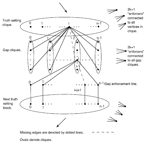
Figure 1: Gadget for Dominating Set

A diagram of the gadget used in the reduction is given in Figure 1. The idea of the proof is as follows. There are $k$ of the gadgets arranged in a circle, where we regard them as ordered from first to last. Each of the gadgets has 3 main parts. Taken clockwise from top to bottom, these are the truth setting clique, the gap selection part (achieved by the gap selection cliques) and the gap enforcement part (achieved by the gap enforcement line).

The pigeonhole principle combined with the so-called enforcers are used to force one vertex from each of the truth cliques and one vertex from each of the next set of cliques, which form the gap enforcement part. The intuition is that the truth selection cliques represent a choice of a particular vertex to be selected to be true, and the gap selection represents the gap till the next selected true vertex. The interconnections between the truth setting cliques and the gap selection means that they align, and the gap enforcement line makes all the selections consistent. Finally because of the clause variables which also need to be dominated, we will ensure that the dominating set corresponds to a truth assignment.

In more detail, the truth selection component is a clique and the gap selection consists of $n$ cliques which we call columns. Our first action is to ensure that in any dominating set of $2k$ elements, we must pick one vertex from each of these two components. This goal is achieved by the $2k$ sets of $2k+1$ enforcers (which are independent sets). For example, for each truth selection clique, $2k+1$ enforcers are connected to every vertex in this clique and nowhere else and then it will follow by the pigeonhole principle that in any size $2k$ dominating set for the final graph, to dominate these enforcers, some vertex in the truth selection clique must be chosen. Similarly, it follows that we must pick exactly one vertex from each of the truth selection cliques, and one of the gap selection cliques to dominate the enforcers.

The truth selection component of the $r$-th gadget is denoted by $A(r)$, $r=0,\ldots,k-1$. Each of these $k$ components consists of a clique of $n$ vertices labeled $0,\ldots,n-1$. The intention is that if the vertex labeled $i$ is picked, this represents variable $i$ being set to true in the formula $X$. We denote by $B(r)$ the gap selection part of the $r$-th gadget, $r=0,\ldots,k-1$. As explained above, this part consists of $n$ columns (cliques) where we index the columns by $i=0,\ldots,n-1$. The intention is that column $i$ corresponds to the choice of variable $i$ in the preceding $A(r)$. The idea then is the following. We join the vertex $a[r,i]$ corresponding to variable $i,$ in $A(r)$, to all vertices in $B(r)$ except those in column $i$. This means that the choice of $i$ in $A(r)$ will cover all vertices of $B(r)$ except those in this column. It follows since we have only $2k$ to spend, that we must choose the dominating element from this column and nowhere else. (There are no connections from column to column.) The columns are meant to be the gap selection saying how many $0$’s there will be till the next positive choice for a variable. We finally need to ensure that if we choose variable $i$ in $A(r)$ and gap $j$ in column $i$ from $B(r)$ then we need to pick $i+j+1$ in $A(r+1)$. This is fulfilled by the gap enforcement component which consists of a set of $n$ vertices. We denote by $d[r,s]$, $s=0,\ldots,n-1$ the set of vertices in this gap-enforcement line in the $r$-th gadget $r=0,\ldots,k-1$.

For $r<k-1$, the method is to connect vertex $j$ in column $i$ of $B(r)$ to all of the $n$ vertices $d[r,s]$ $except$ to $d[r,i+j+1]$ provided that $i+j+1\leq n$. (For $r=k-1$ simply connect vertex $j$ in column $i$ of $B(r)$ to all of the $n$ vertices $d[r,s]$ except to $d[r,i+j+1]$ since this will need to “wrap around” to $A(0)$.) The first point of this process is that if we choose vertex $j$ in column $i$ with $i+j+1>n$ then none of the vertices in the enforcement line are dominated. Since there is only a single edge to the corresponding vertex in $A(r+1)$, there cannot possibly be a size $2k$ dominating set for such a choice. It follows that we must choose some $j$ with $i+j+1\leq n$ in any dominating set of size $\leq 2k$. The main point is that if we choose $j$ in column $i$ we will dominate all of the $d[r,s]$ except $d[r,i+j+1]$. Since we will only connect $d[r,s]$ additionally to $a[r+1,s]$ and nowhere else, to choose an element of $A[r+1]$ and still dominate all of the $d[r,s]$ we must actually choose $a[r+1,i+j+1]$.

Thus the above provides a selection gadget that chooses $k$ true variables with the gaps representing false ones. We enforce that the selection is consistent with the clauses of $X$ via clause vertices $c_{i}$ one for each clause $C_{i}$. These are connected in the obvious ways. One connects a choice in $A[r]$ or $B[r]$ corresponding to making a clause $C_{q}$ true to the vertex $c_{q}$. Then if we dominate all the clause variables too, we must have either chosen in some $A[r]$ a positive occurrence of a variable in $C_{q}$ or we must have chosen in $B[r]$ a gap corresponding to a negative occurrence of a variable in $C_{q}$, and conversely. The formal details can be found in Downey and Fellows [122, 125].∎

There are notable problems which are ${\sf W}[t]$-hard for all $t$, such as Bandwidth, below.

Bandwidth
Instance: A graph $G=(V,E)$.
Parameter: A positive integer $k$.
Question: Is there a 1-1 layout $f:V\to\{1,\dots,|V|\}$ such that $\{u,v\}\in E$ implies $|f(u)-f(v)|\leq k$?

The $W[t]$ (for all $t$) hardness of Bandwidth was proven by Bodlaender, Fellows and Hallett [36] via a rather complex reduction. It is unknown what, say, Bandwidth $\in{\sf W}[1]$ (or even ${\sf W}[{\sf P}]$) would imply either parametrically or classically. On general grounds, it seems unlikely that such a containment is possible.

At even higher levels, we can define Weighted Sat to be the weighted satisfiability problem where inputs correspond to unrestricted Boolean formulas and finally Weighted Circuit Sat to be the most general problem whose inputs are all polynomial sized circuits.

Notice that, in Theorem 3.2, we did not say that Weighted CNF Sat is ${\sf W}[1]$-complete. The reason for this is that we do not believe that it is! In fact, we believe that ${\sf W}[2]\neq{\sf W}[1].$

That is, classically, using a padding argument, we know that CNF Sat $\equiv_{m}^{P}$ $3$CNF Sat. However, the classical reduction does not define a parameterized reduction from Weighted CNF Sat to Weighted $3$CNF Sat, it is not structure-preserving enough to ensure that parameters map to parameters. In fact, it is conjectured [122] that there is no parameterized reduction at all from Weighted CNF Sat to Weighted $3$CNF Sat. If the conjecture is correct, then Weighted CNF Sat is not in the class ${\sf W}[1]$.

The point here is that parameterized reductions are more refined than classical ones, and hence we believe that we get a wider variety of apparent hardness behaviour when intractable problems are classified according to this more fine-grained analysis.

These classes form part of the basic hierarchy of parameterized problems below.

$${\sf FPT}\subseteq{\sf W}[1]\subseteq{\sf W}[2]\subseteq\cdots\subseteq{\sf W}[t]\subseteq{\sf W}[SAT]\subseteq{\sf W}[{\sf P}]\subseteq{\sf AW}[t]\subset{\sf AW}[{\sf P}]\subseteq{\sf{\sf XP}}$$

This sequence is commonly termed “the ${\sf W}$-hierarchy”. The complexity class ${\sf W}[1]$ can be viewed as the parameterized analog of NP, since it suffices for the purpose of establishing likely parameterized intractability.

The classes ${\sf W}[SAT]$, ${\sf W}[{\sf P}]$ and the ${\sf AW}$ classes were introduced by Abrahamson, Downey and Fellows in [2]. The class ${\sf W}[SAT]$ is the collection of parameterized languages ${\sf FPT}$-reducible to Weighted Sat. The class ${\sf W}[{\sf P}]$ is the collection of parameterized languages FPT-equivalent to Weighted Circuit Sat, the weighted satisfiability problem for a decision circuit $C$ that is unrestricted. A standard translation of Turing machines into circuits shows that $K$-Weighted Circuit Sat is the same as the problem of deciding whether or not a deterministic Turing machine accepts an input of weight $k$. It is conjectured that the containment ${\sf W}[SAT]\subseteq{\sf W}[{\sf P}]$ is proper [125].

Another way to view ${\sf W}[{\sf P}]$ is the following. Consider the problem Short Circuit Sat defined as follows.

Short Circuit Sat
Instance: A decision circuit $C$ with at most $n$ gates and $k\log n$ inputs.
Parameter: A positive integer $k$.
Question: Is there a setting of the inputs making $C$ true?

Theorem 3.6 (Abrahamson, Downey and Fellows [2]).

Short Circuit Sat is ${\sf W}[{\sf P}]$-complete.

Proof.

The proof of this result uses the “$k\cdot\log n$” trick introduced by Abrahamson, Downey and Fellows [2]. To see that the problem is ${\sf W}[{\sf P}]$-hard, take an instance $I$ of Weighted Circuit Satisfiability with parameter $k$ and inputs $x_{1},\dots,x_{n}$. Let $z_{1},\dots,z_{k\log n}$ be new variables. Using lexicographic order and in polynomial time we have a surjection from this set to the $k$-element subsets of $x_{1},\dots,x_{n}$. Representing this as a circuit and putting this on the top of the circuit for $I$ defines our new circuit $C$. The converse is equally easy.∎

${\sf AW}[t]$ captures the notion of alternation. ${\sf AW}[t]$ is the collection of parameterized languages ${\sf FPT}$-reducible to Parameterized Quantified Circuit Sat_t, the weighted satisfiability problem for an unrestricted decision circuit that applies alternating quantifiers to the inputs, defined here.

Parameterized Quantified Circuit Sat_t

Instance:  A weft $t$ decision circuit $C$ whose inputs correspond to a sequence $s_{1},\ldots s_{r}$ of pairwise disjoint sets of variables.
Parameter: $r,\;k_{1},\ldots,k_{n}$.
Question:  Is it the case that there exists a size $k_{1}$ subset $t_{1}$ of $s_{1}$, such that for every size $k_{2}$ subset $t_{2}$ of $s_{2}$, there exists a size $k_{3}$ subset $t_{3}$ of $s_{3}$, such that $\ldots$ (alternating quantifiers) such that, when $t_{1}\cup t_{2}\cup\ldots\cup t_{r}$ are set to true, and all other variables are set to false, $C$ is satisfied?

The idea here is to look at the analog of PSPACE. The problem is that in the parameterized setting there seems no natural analog of Savitch’s Theorem or the proof that QBFSat is PSPACE-complete, and it remains an interesting problem to formulate a true analog of parameterized space.

The approach taken by [2] was to look at the parameterized analog of QBFSat stated above.

One of the fundamental theorems proven here is that the choice of $t$ is irrelevant:

Theorem 3.7 (Abrahamson, Downey and Fellows [2]).

${\sf AW}[t]={\sf AW}[1]$ for all $t\geq 1$.

Many parameterized analogs of game problems are complete for the ${\sf AW}[1]$, such as the parameterized analog of Geography.

Short Geography
Instance: A directed graph $D=(V,E)$ and a specified vertex $v_{0}$.
Parameter: A positive Integer $k$.
Question: Does player 1 have a winning strategy in the following game? Each player alternatively chooses a new arc from $E$. The first arc must have its tail as $v_{0}$, and each vertex subsequently chosen must have as its tail the head of the previously chosen arc. The first player unable to choose loses.

The class ${\sf XP}$, introduced in [125], is the collection of parameterized languages $L$ such that the $k$-th slice of $L$ (the instances of $L$ having parameter $k$) is a member of ${\sf DTIME}(n^{k})$. ${\sf XP}$ is provably distinct from ${\sf FPT}$ and seems to be the parameterized class corresponding to the classical class ${\sf EXP}$ (exponential time). There are problems complete for ${\sf XP}$ including the game of $k$-Cat and Mice. The problem here is played on a directed graph $G=(V,E)$ and begins with a distinguished vertex $v_{0}$ called the cheese, a token $c$ on one vertex called the cat, and $k$ tokens (called mice) on other vertices. Players cat and the team of mice play alternatively moving one token at a time. A player can move a token along an arc at each stage. Team of mice wins if one mouse can reach the cheese (by occupying it even if the cat is already there) before the cat can eat one of the mice by occupying the same vertex.

It is conjectured that all of the containments given so far are proper, but all that is currently known is that FPT is a proper subset of ${\sf XP}$.

There are hundreds of complete problems for the levels of the hierarchy. Here is a short list. The reader is referred to [116] for references and definitions. As stated ${\sf XP}$ has $k$-Cat and Mouse Game and many other games; ${\sf W}[{\sf P}]$ has Linear Inequalities, Short Satisfiability, Weighted Circuit Satisfiability and Minimum Axiom Set. There are a number of quite important problems from combinatorial pattern matching which are ${\sf W}[t]$ hard for all $t$: Longest Common Subsequence ($k=$ number of sequences, $|\Sigma|$-two parameters), Feasible Register Assignment, Triangulating Colored Graphs, Bandwidth, Topological Bandwidth, Proper Interval Graph Completion, Domino Treewidth and Bounded Persistence Pathwidth. Some concrete problems complete for ${\sf W}[2]$ include Weighted $\{0,1\}$ Integer Programming, Dominating Set, Tournament Dominating Set, Unit Length Precedence Constrained Scheduling (hard), Shortest Common Supersequence (hard), Maximum Likelihood Decoding (hard), Weight Distribution in Linear Codes (hard), Nearest Vector in Integer Lattices (hard), Short Permutation Group Factorization (hard). Finally a collection of ${\sf W}[1]$-complete problems: $k$-Step Derivation for Context Sensitive Grammars, Short NTM Computation, Short Post Correspondence, Square Tiling, Weighted $q$–CNF Satisfiability, Vapnik–Chervonenkis Dimension, Longest Common Subsequence ($k$, $m=$ length of common subseq.), Clique, Independent Set, and Monotone Data Complexity for Relational Databases. This list is merely representative, and new areas of application are being found all the time. There are currently good compendia of hardness and completeness results as can be found at the web

http://bravo.ce.uniroma2.it/home/cesati/research/compendiuma/

For older material, see the appendix of the monograph by Downey and Fellows [125], as well as the many surveys and the recent issue of the Computer Journal [128].

There remain several important structural questions associated with the ${\sf W}$-hierarchy such as how it relates to the ${\sf A}$-hierarchy below, and whether any collapse may propagate.

Open questions : Does ${\sf W}[t]={\sf W}[t+1]$ imply ${\sf W}[t]={\sf W}[t+2]$? Does ${\sf W}[t]={\sf FPT}$ imply ${\sf W}[t+1]={\sf FPT}?$

3.4 The ${\sf A}$-hierarchy and the Flum-Grohe approach

There have been several attempts towards simplification of this material, notably by Flum and Grohe [154]. Their method is to try to make the use of logical depth and logic more explicit. To do this Flum and Grohe take a detour through the logic of finite model theory. Close inspection of their proofs reveals that similar combinatorics are hidden. Their view is that model checking should be viewed as the fundamental viewpoint of complexity.

To this end, for a class of first order formula $\varphi$ with $s$-ary free relation variable, we can define $p\mbox{-\sc WD}(\varphi)$ as the problem:

$p\mbox{-\sc WD}(\varphi)$
Instance: A structure ${\mathcal{A}}$ with domain $A$ and an integer $k$.
Parameter: $k$.
Question: Is there a relation $R\subseteq A^{s}$ with $|R|=k$ such that ${\mathcal{A}}\vDash\varphi(R)?$

This idea naturally extends to classes $\Phi$ of formulae $\Phi$. Then we define $p\mbox{-\sc WD}(\Phi)$ to be the class of parameterized problems $p\mbox{-\sc WD}(\varphi)$ for $\varphi\in\Phi$. It is easy to show that $p\mbox{-\sc WD}({\Sigma_{1}})={\sf FPT}.$ (Strictly, we should write $\Sigma_{1}^{0}$ but the formulae considered here are first order.) Then to recast the classical ${\sf W}$-hierarchy at the finite levels, the idea is to define for $t\geq 1$,

$${\sf W}[t]=[p\mbox{-\sc WD}({\Pi_{t}})]^{{\sf FPT}},$$

where, given a parameterized problem $X$, $[X]^{{\sf FPT}}$ denotes the parameterized problems that are ${\sf FPT}$-reducible to $X$.

Flum and Grohe have similar logic-based formulations of the other W-hierarchy classes. We refer the reader to [154] for more details.

We remark that the model checking approach leads to other hierarchies. One important hierarchy found by Flum and Grohe is the ${\sf A}$-hierarchy which is also based on alternation like the AW-hierarchy but works differently. For a class $\Phi$ of formulae, we can define the following parameterized problem.

$p\mbox{\sc-MC}(\Phi)$
Instance: A structure ${\mathcal{A}}$ and a formula $\varphi\in\Phi$.
Parameter: $|\varphi|$.
Question: Decide if $\phi({\mathcal{A}})\neq\emptyset,$ where this denotes the evaluation of $\phi$ in ${\mathcal{A}}$.

Then Flum and Grohe define

$${\sf A}[t]=[p\mbox{\sc-MC}(\Sigma_{t})]^{{\sf FPT}}.$$

For instance, for $k\geq 1$, $k$-Clique can be defined by

$$\mbox{clique}_{k}=\exists x_{1},\dots x_{k}(\bigwedge_{1\leq i<j\leq k}x_{i}\neq x_{j}\land\bigwedge_{1\leq i<j\leq k}Ex_{i}x_{j})$$

in the language of graphs, and the interpretation of the formula in a graph $G$ would be that $G$ has a clique of size $k$. Thus the mapping $(G,k)\mapsto(G,\mbox{clique}_{k})$ is a FPT reduction showing that parameterized Clique is in ${\sf A}[1].$ Flum and Grohe populate various levels of the $A$-hierarchy and show the following.

Theorem 3.8 (Flum and Grohe [154]).

The following hold:

• ${\sf A}[1]={\sf W}[1].$

• ${\sf A}[t]\subseteq{\sf W}[t]$.

Clearly ${\sf A}[t]\subseteq{\sf XP}$, but no other containment with respect to other classes of the ${\sf W}$-hierarchy is known. It is conjectured by Flum and Grohe that no other containments than those given exist, but this is not apparently related to any other conjecture.

If we compare classical and parameterized complexity it is evident that the framework provided by parameterized complexity theory allows for more finely-grained complexity analysis of computational problems. It is deeply connected with algorithmic heuristics and exact algorithms in practice. We refer the reader to either the survey [154], or those in two recent issues of The Computer Journal [128] for further insight.

We can consider many different parameterizations of a single classical problem, each of which leads to either a tractable, or (likely) intractable, version in the parameterized setting. This allows for an extended dialog with the problem at hand. This idea towards the solution of algorithmic problems is explored in, for example, [131]. A nice example of this extended dialog can be found in the work of Iris van Rooij and her co-authors, as discussed in van Rooij and Wareham [278].

3.5 Connection with PTAS’s

The reader may note that parameterized complexity is addressing intractability within polynomial time. In this vein, the parameterized framework can be used to demonstrate that many classical problems that admit a PTAS do not, in fact, admit any PTAS with a practical running time, unless ${\sf W}[1]={\sf FPT}$. The idea here is that if a ${\sf PTAS}$ has a running time such as $O(n^{\frac{1}{\epsilon}})$, where $\epsilon$ is the error ratio, then the PTAS is unlikely to be useful. For example if $\epsilon=0.1$ then the running time is already $n$ to the 10th power for an error of $10\%$. What we could do is regard $\frac{1}{\epsilon}$ as a parameter and show that the problem is ${\sf W}[1]$-hard with respect to that prameterization. In that case there would likely be no method of removing the $\frac{1}{\epsilon}$ from the exponent in the running time and hence no efficient PTAS, a method first used by Bazgan [25]. For many more details of the method we refer the reader to the survey [116].

A notable application of this technique is due to Cai et. al. [51] who showed that the method of using planar formulae tends to give PTAS’s that are never practical. The exact calibration of PTAS’s and parameterized complexity comes through yet another hierarchy called the ${\sf M}$-hierarchy. The breakthrough was the realization by Cai and Juedes [53] that the collapse of a basic sub-hierarchy of the ${\sf W}$-hierarchy was deeply connected with approximation.

The base level of the hierarchy is the problem ${\sf M}[1]$ defined by the core problem below.

Instance: A CNF circuit $C$ (or, equivalently, a CNF formula) of size $k\log n$.
Parameter: A positive integer $k$.
Question: Is $C$ satisfiable?

That is, we are parameterizing the size of the problem rather than some aspect of the problem. The idea naturally extends to higher levels for that, for example, M[2] would be a product of sums of product formula of size $k\log n$ and we are asking whether it is satisfiable.

The basic result is that ${\sf FPT}\subseteq{\sf M}[1]\subseteq{\sf W}[1]$. The hypothesis ${\sf FPT}\neq{\sf M}[1]$ is equivalent to ETH. In fact, as proven in [76], there is an isomorphism, the so-called miniaturization, between exponential time complexity (endowed with a suitable notion of reductions) and XP (endowed with FPT reductions) such that the respective notions of tractability correspond, that is, subexponential time on the one and FPT on the other side. The reader might wonder why we have not used a Turing Machine of size $k\log n$ in the input, rather than a CNF circuit. The reason is that whilst we can get reductions for small version of problems, such as $k\log n$-Vertex Cover and the like, to have the same complexity as the circuit problem above, we do not know how to do this for Turing machines. It remains an open question whether the $k\log n$-sized circuit problem and the $k\log n$-sized Turing Machine problem have the same complexity.

For more on this topic and other connections with classical exponential algorithms we refer the reader to the survey of Flum and Grohe [154].

3.6 FPT and XP optimality

Related to the material of the last section are emerging programmes devoted to proving tight lower bounds on parameterized problems, assuming various non-collapses of the parameterized hierarchies. For this section, it is useful to use the $O^{*}$ notation for parameterized algorithms. This is the part of the running time which is exponential. For example, a running time of $2^{k^{2}}|G|^{5}$ would be written as $O^{*}(2^{k^{2}}).$

One example of a lower bound was the original paper of Cai and Juedes [53, 54] who proved the following definitive result.

Theorem 3.9.

$k$-Planar Vertex Cover, $k$-Planar Independent Set, $k$-Planar Dominating Set, and $k$-Planar Red/Blue Dominating Set cannot be in $O^{*}(2^{o(\sqrt{k})})$-${\sf FPT}$ unless ${\sf FPT}={\sf M}[1]$ (or, equivalently, unless ETH fails).

The optimality of Theorem 3.9 follows from the fact that all above problems have been classified in $O^{*}(2^{O(\sqrt{k})})$-FPT as proved in [8, 207, 165, 210] (see also Subsection 4.3.3).

We can ask for similar optimality results for any FPT problem. See for example, Chen and Flum [74]. We will meet another approach to FPT optimality in Subsection 3.11 where we look at classes like EPT meant to capture how problems are placed in FPT via another kind of completeness programme.

Another example of such optimality programmes can be found in exciting resent work on XP optimiality. This programme represents a major step forward in the sense that it regards the classes like ${\sf W}[1]$ as artifacts of the basic problem of proving hardness under reasonable assumptions, and strikes at membership of ${\sf XP}$.

Here are some examples. We know that Independent Set and Dominating Set are in ${\sf XP}$.

Theorem 3.10 (Chen et. al [62]).

The following hold:

• Independent Set cannot be solved in time $n^{o(k)}$ unless ${\sf FPT}={\sf M}[1].$

• Dominating Set cannot be solved in time $n^{o(k)}$ unless ${\sf FPT}={\sf M}[2]$.

A beautiful development in this area is the resent paper by Marx on the Closest Substring problem. We refer to Marx [223] for more details, and to Chen and Meng [72] for other related results.

There remains a lot of work to be done here and these programmes appear to be exciting developments, see e.g., [159, 157, 220, 219].

3.7 Other classical applications

Similar techniques have been used to solve a significant open question about techniques for formula evaluation when they were used to show “resolution is not automizable” unless ${\sf W}[{\sf P}]={\sf FPT}$ (Alekhnovich and Razborov [13], Eickmeyer, Grohe and Grüber [137].) Parameterized complexity assumptions can also be used to show that the large hidden constants (various towers of two’s) in the running times of generic algorithms obtained though the use of algorithmic meta-theorems cannot be improved upon (see [155].) One illustration is obtained through the use of local treewidth (which we will discuss in Subection 4.2.2). The notions of treewidth and branchwidth are by now ubiquitous in algorithmic graph theory (the definition of branchwidth is given in Subsection 4.2.1). Suffice to say is that it is a method of decomposing graphs to measure how “treelike” they are, and if they have small treewidth/branchwidth, as we see in Subection 4.2.1, we can run dynamic programming algorithms upon them. The local treewidth of a class ${\mathcal{C}}$ of graphs is called bounded iff there a function $f$ such that for all graphs $G\in{\mathcal{C}}$ and all vertices $v\in V(G)$ the neighborhood of $v$ of distance $k$ from $v$ has treewidth $f(k)$ (see Subsection 4.2.2). Examples include planar graphs and graphs of bounded maximum degree. The point is that a class of graphs of bounded local treewidth is automatically FPT for a wide class of properties.

Theorem 3.11 (Frick and Grohe [169]).

Deciding first-order statements is FPT for every fixed class of graphs of bounded local treewidth.

One problem with this algorithmic meta-theorem is that the algorithm obtained for a fixed first-order statement $\varphi$ can rapidly have towers of twos depending on the quantifier complexity of the statement, in the same way that this happens for Courcelle’s theorem on decidability of monadic second order statements (as discussed in Subsection 4.2.1) for graphs of bounded treewidth. What Frick and Grohe [170] showed is that such towers of two’s cannot be removed unless ${\sf W}[{\sf P}]={\sf FPT}.$

Another use of parameterized complexity is to give an indirect approach to proving likely intractability of problems which are not known to be NP-complete. A classic example of this is the following problem.

Precedence Constrained $k$-Processor Scheduling
Instance: A set $T$ of unit-length jobs and a partial ordering $\preceq$ on $T$, a positive deadline $D$ and a number of processors $k$.
Parameter: A positive integer $k$.
Question: Is there a mapping $f:T\to\{1,\dots,D\}$ such that for all $t\prec t^{\prime}$, $f(t)\prec f(t^{\prime})$, and for all $i$, $1\leq i\leq D$, $|f^{-1}(i)|\leq k?$.

In general this problem is NP-complete and is known to be in P for 2 processors. The question is what happens for $k>2$ processors. For us the question becomes whether the problem is in XP for $k>2$ processors. This remains one of the open questions from Garey and Johnson’s famous book [172] (Open Problem 8), but we have the following.

Theorem 3.12 (Bodlaender, Fellows and Hallett [36]).

Precedence Constrained $k$-Processor Scheduling is ${\sf W}[2]$-hard.

The point here is that even if  Precedence Constrained $k$-Processor Scheduling is in XP, there seems no way that it will be feasible for large $k$. Researchers in the area of parameterized complexity have long wondered whether this approach might be applied to other problems like Composite Number or Graph Isomorphism. For example, Luks [222] has shown that Graph Isomorphism can be solved in $O(n^{k})$ for graphs of maximum degree $k$, but any proof that the problem was ${\sf W}[1]$ hard would clearly imply that the general problem was not feasible. We know that Graph Isomorphism is almost certainly not NP-complete, since proving that would collapse the polynomial hierarchy to 2 or fewer levels (see the work of Schöning in [262]). Similar comments can be applied to graphs of bounded treewidth by Bodlaender [33].

3.8 Other parameterized classes

There have been other parameterized analogs of classical complexity analyzed. For example McCartin [227] and Flum and Grohe [153] each analyzed parameterized counting complexity. Here we can define the class $\#{\sf W}[1]$ for instance (with the core problem being counting the number of accepting paths of length $k$ in a nondeterministic Turing machine), and show that counting the number of $k$ cliques is $\#{\sf W}[1]$-complete. Notably Flum and Grohe proved the following analog to Valiant’s Theorem on the permanent.

Theorem 3.13 (Flum and Grohe [153]).

Counting the number of cycles of size $k$ in a bipartite graph is $\#{\sf W}[1]$-complete.

One of the hallmark theorems of classical complexity is Toda’s Theorem which states that ${\sf P}^{\#{\sf P}}$ contains the polynomial time hierarchy. There is no known analog of this result for parameterized complexity. One of the problems is that all known proofs of Toda’s Theorem filter through probabilistic classes. Whilst there are known analogs of Valiant’s Theorem (Downey, Fellows and Regan [130], and Müller [230, 231]), there is no known method of “small” probability amplification. (See Montoya [229] for a thorough discussion of this problem.) This seems the main problem and there is really no satisfactory treatment of probability amplification in parameterized complexity. For example, suppose we wanted an analog of the operator calculus for parameterized complexity. For example, consider ${\sf BP}\cdot\oplus{\sf W}[{\sf P}]$, as an analog of ${\sf BP}\cdot\oplus{\sf P}$. We can define $L\in\oplus{\sf W}[{\sf P}]$ to mean that $(x,k)\in L$ iff $(x,k)\mapsto(x^{\prime},k^{\prime})$ where $x^{\prime}$ is a circuit with (e.g.) $k\log|x^{\prime}|$ inputs and the number of accepting inputs is odd. We need that there is a language $L\in{\sf BP}\cdot{\mathcal{C}}$ iff there is a language $L^{\prime}\in{\mathcal{C}}$ such that for all $(x,k)$,

$$(x,k)\in L\mbox{ iff a randomly chosen }(x,k,k^{\prime})\in L^{\prime}.$$

A problem will appear as soon as we try to prove the analog basic step in Toda’s Theorem: ${\sf W}[{\sf P}]\subseteq{\sf BP}\cdot\oplus{\sf W}[{\sf P}].$ The first step in the usual proof of Toda’s Theorem, which can be emulated, is to use some kind of random hashing to result in a $\oplus{\sf W}[{\sf P}]$ circuit with either no accepting inputs, or exactly one accepting input, the latter with nonzero probability. So far things work out okay. However, the next step in the usual proof is to amplify this probability: that is, do this a polynomial number of times independently to amplify by majority to get the result in the ${\sf BP}$ class. The problem is that if this amplification uses many independently chosen instances, then the number of input variables goes up and the the result is no longer a ${\sf W}[{\sf P}]$ circuit since we think of this as a polynomial sized circuit with only $k\log n$ many inputs. There is a fundamental question: Is it possible to perform amplification with only such limited nondeterminism?

Notable here are the following:

Theorem 3.14 (Downey, Fellows and Regan [130]).

For all $t$, there is a randomized FPT-reduction from ${\sf W}[t]$ to unique ${\sf W}[t]$. (Analog of of the Valiant-Vaziarini Theorem)

Theorem 3.15 (Müller [232]).

${\sf W}[{\sf P}]\cdot{\sf BPFPT}$ (an analog of ${\sf BPP}$) has weakly uniform derandomization (“weakly uniform” is an appropriate technical condition) iff there is a polynomial time computable unbounded function $c:{\mathbb{N}}\to{\mathbb{N}}$ with ${\sf BPP}(c)={\sf P}$, where ${\sf BPP}(c)$ denotes BPP with only access to $c(n)\log n$ nondeterministic bits.

Moritz Müller’s result says that, more or less, parameterized derandomization implies nontrivial classical derandomization. Other interesting work on randomization in parameterized complexity is to be found in the work of Müller. For instance, in [230], he showed that there is a Valiant-Vaziarini type lemma for most ${\sf W}[t]$-complete problems, including e.g. Unique Dominating Set. The only other work in this area is in the papers of Montoya, such as [229]. In [229], Montoya showed that it is in a certain sense unlikely that BP$\cdot$W[P], an analogue of the classical Arthur-Merlin class, allows probability amplification. (That is, amplification with $k\log n$ bits of nodeterminism is in a sense unlikely.) Much remains to do here.

Perhaps due to the delicacy of material, or because of the focus on practical computation, there is only a little work on what could be called parameterized structural complexity. By this we mean analogs of things like Ladner’s Theorem (that if $P\neq NP$ then there are sets of intermediate complexity) (See [117]), Mahaney’s Theorem that if there is a sparse $NP$ complete set then $P=NP$ (Cesarti and Fellows [58], the PCP Theorem, Toda’s theorem etc. There is a challenging research agenda here.

3.9 Parameterized approximation

One other fruitful area of research has been the area of parameterized approximation, beginning with three papers at the same conference! (Cai and Huang [52], Chen, Grohe and Grüber [77], and Downey, Fellows and McCartin [118]). Parameterized approximation was part of the folklore for some time originating with the dominating set question originally asked by Fellows. For parameterized approximation, one inputs a problem and asks for either a solution of size $f(k)$ or a statement that there is no solution of size $k$. This idea was originally suggested by Downey and Fellows, inspired by earlier work of Robertson and Seymour on approximations to treewidth. Of course, we need to assume that ${\sf FPT}\neq{\sf W}[1]$ for this to make sense. A classical example taken from Garey and Johnson [172] is Bin Packing where the First Fit algorithm either says that no packing of size $k$ exists or gives one of size at most $2k$. As observed by Downey, Fellows and McCartin [118] most ${\sf W}[t]$ hard problems do not have approximations with an additive factor (i.e. $f(k)=k+c$) unless ${\sf W}[t]={\sf FPT}.$ One surprise from that paper is the following.

Theorem 3.16 (Downey, Fellows, McCartin [118]).

The problem Independent Dominating Set which asks if there is a dominating set of size $k$ which is also an independent set, has no parameterized approximation algorithm for any computable function $f(k)$ unless ${\sf W}[2]={\sf FPT}.$

Subsequently, Eickmeyer, Grohe Grüber showed the following in [137].

Theorem 3.17.

If $L$ is a “natural” ${\sf W}[{\sf P}]$-complete language then $L$ has no parameterized approximation algorithm unless ${\sf W}[{\sf P}]={\sf FPT}.$

The notion of “natural” here is indeed quite natural and covers all of the known ${\sf W}[{\sf P}]$-complete problems, say, in the appendix of Downey and Fellows [125]. We refer the reader to [137] for more details.

One open question asks whether there is any multiplicative FPT approximation for Dominating Set. This question of Mike Fellows has been open for nearly 20 years and asks in its oldest incarnation whether there is an algorithm which, on input $(G,k)$ either says that there is no size $k$ dominating set, or that there is one of size $2k$.

3.10 Limits on kernelization

There has been important recent work concerning limitations of parameterized techniques. One of the most important techniques is that of kernelization. We will see in Subsection 4.4 that this is one of the basic techniques of the area, and remains one of the most practical techniques since usually kernelization is based around simple reduction rules which are both local and easy to implement. (See, for instance Abu-Khzam, et. al. [4], Flum and Grohe [154], or Guo and Niedermeier [185].) The idea, of course, is that we shrink the problem using some polynomial time reduction to a small one whose size depends only on the parameter, and then do exhaustive search on that kernel. Naturally the latter step is the most time consuming and the problem becomes how to find small kernels. An important question is therefore: When is it possible to show that a problem has no polynomial kernel? A formal definition of kernelization is the following:

Definition 3.18 (Kernelization).

A kernelization algorithm, or in short, a kernel for a parameterized problem $L\subseteq\Sigma^{*}\times\mathbb{N}$ is an algorithm that given $(x,k)\in\Sigma^{*}\times\mathbb{N}$, outputs in $p(|x|+k)$ time a pair $(x^{\prime},k^{\prime})\in\Sigma^{*}\times\mathbb{N}$ such that

• $(x,k)\in L\Leftrightarrow(x^{\prime},k^{\prime})\in L$,

• $(|x^{\prime}|,k^{\prime})\leq f(k)$,

where $f$ is an arbitrary computable function, and $p$ a polynomial. Any function $f$ as above is referred to as the size of the kernel. We frequently use the term “kernel” for the outputs $(|x^{\prime}|,k^{\prime})$ of the kernelization algorithm and, in case $f$ is a polynomial (resp. linear) function, we say that we have a polynomial (resp. linear) kernelization algorithm or, simply, a polynomial (resp. linear) kernel.

Clearly, if ${\sf P}={\sf NP}$, then all problems have constant size kernels so some kind of complexity theoretical hypothesis is needed to show that something does not have a small kernel. The key thing that the reader should realize is that the reduction to the kernel is a polynomial time reduction for both the problem and parameter, and not an FPT algorithm. Limiting results on kernelization mean that this often used practical method cannot be used to get FPT algorithms. Sometimes showing that problems do not have small kernels (modulo some hypothesis) can be extracted from work on approximation, since a small kernel is, itself, an approximation. Thus, whilst we know of a $2k$ kernel for $k$-Vertex Cover [234], we know that unless ${\sf P}={\sf NP}$, we cannot do better than size $1.36\cdot k$ using Dinur and Safra [107], since the PCP theorem provides a 1.36-lower bound on approximation (see also [185]).

To show that certain problems do not have polynomial kernels modulo a reasonable hypothesis, we will need the following definition, which is in classical complexity. (It is similar to another definition of Harnik and Noar [189]).

Definition 3.19 (Or-Distillation).

An Or-distillation algorithm for a classical problem $L\subseteq\Sigma^{*}$ is an algorithm that

• receives as input a sequence $(x_{1},\ldots,x_{t})$, with $x_{i}\in\Sigma^{*}$ for each $1\leq i\leq t$,

• uses time polynomial in $\sum_{i=1}^{t}|x_{i}|$,

• and outputs a string $y\in\Sigma^{*}$ with

  1. $y\in L\iff x_{i}\in L$ for some $1\leq i\leq t$.

  2. $|y|$ is polynomial in $\max_{1\leq i\leq t}|x_{i}|$.

We can similarly define And-distillation by replacing the second last item by “$y\in L\iff x_{i}\in L$ for all $1\leq i\leq t$.” Bodlaender, Downey, Fellows and Hermelin [35] showed that an NP-complete problem has an Or-distillation algorithm iff all of them do. On general Kolmogorov complexity grounds, it seems very unlikely that NP-complete problems have either distillation algorithms. Following a suggestion of Bodlaender, Downey, Fellows and Hermelin, Fortnow and Santhanam related Or-distillation to the polynomial time hierarchy as follows.

Lemma 3.20 ([167]).

If any NP-complete problem has an Or-distillation algorithm then co-${\sf NP}\subseteq{\sf NP}\backslash$Poly and hence the polynomial time hierarchy collapses to 3 or fewer levels.

At the time of writing, there is no known version of Lemma 3.20 for And-distillation and it remains an important open question, whether NP-complete problems having And-distillation implies any classical collapse of the polynomial time hierarchy. This material all relates to kernelization as follows.

Definition 3.21 (Composition).

An Or-composition algorithm for a parameterized problem $L\subseteq\Sigma^{*}\times\mathbb{N}$ is an algorithm that

• receives as input a sequence $((x_{1},k),\ldots,(x_{t},k))$, with $(x_{i},k)\in\Sigma^{*}\times\mathbb{N}^{+}$ for each $1\leq i\leq t$,

• uses time polynomial in $\sum_{i=1}^{t}|x_{i}|+k$,

• and outputs $(y,k^{\prime})\in\Sigma^{*}\times\mathbb{N}^{+}$ with

  1. $(y,k^{\prime})\in L\iff(x_{i},k)\in L$ for some $1\leq i\leq t$.

  2. $k^{\prime}$ is polynomial in $k$.

Again we may similarly define And-composition. The key lemma relating the two concepts is the following, which has an analogous statement for the And-distillation case:

Lemma 3.22 (Bodlaender, Downey, Fellows and Hermelin [35]).

Let $L$ be a Or-compositional parameterized problem whose unparameterized version $\widetilde{L}$ is NP-complete. If $L$ has a polynomial kernel, then $\widetilde{L}$ is also Or-distillable.

Distillation of one problem within another has also been discussed in Chen, Flum and Müller [35].

Using Lemma 3.22, Bodlaender, Downey, Fellows and Hermelin [35] proved that a large class of graph-theoretic FPT problems including $k$-Path, $k$-Cycle, various problems for graphs of bounded treewidth, etc., all have no polynomial-sized kernels unless the polynomial-time hierarchy collapses to three or fewer levels.

For And-composition, tying the distillation to something like the Fortnow-Santhanam material would be important since it would say that important FPT problems like Treewidth and Cutwidth would likely not have polynomial size kernels, and would perhaps suggest why algorithms such as Bodlaender’s linear time FPT algorithm [34] (and other treewidth algorithms) is so hard to run. Since the original paper [35], there have been a number of developments such as the Bodlaender, Thomassé, and Yeo [43] use of reductions to extend the arguments above to wider classes of problems such as Disjoint Paths, Disjoint Cycles, and Hamilton Cycle Parameterized by Treewidth. In the same direction, Chen, Flum and Müller [75] used this methodology to further explore the possible sizes of kernels. One fascinating application was by Fernau et. al. [151]. They showed that the following problem was in FPT, by showing a kernel of size $O(k^{3})$.

Rooted $k$-OutLeaf Branching
Instance: A directed graph $D=(V,E)$ with exactly one vertex of indegree $0$ called the root.
Parameter: A positive integer $k$.
Question: Is there an oriented subtree $T$ of $D$ with exactly $k$ leaves spanning $D$?

However, for the unrooted version they used the machinery from  [35] to demonstrate that it has no polynomial-size kernel unless some collapse occurs, but clearly by using $n$ independent versions of the rooted version the problem has a polynomial-time Turing kernel. We know of no method of dealing with the non-existence of polynomial time Turing kernels and it seems an important programmatic question.

All of the material on lower bounds for Or distillation tend to use reductions to things like large disjoint unions of graphs having Or composition. Thus, problems sensitive to this seemed not readily approachable using the machinery. Very recently, Stefan Kratsch [211] discovered a way around this problem using the work Dell and van Melkebeek [92].

Theorem 3.23 (Kratsch [211]).

The FPT problem $k$-Ramsey which asks if a graph $G$ has either an independent set or a clique of size $k$, has no polynomial kernel unless NP$\subseteq co-NP\backslash$poly.

The point here is that a large collection of disjoint graphs would have a large independent set, hence new ideas were definitely needed. The ideas in Kratsch’s proof are quite novel and use co-nondetermism in compositions and communication complexity in a quite novel way. Perhaps they might allow us to attack other such problems.

Finally, we remark in passing that as an important spinoff of the question from parameterized complexity, the Fortnow-Santhanam Lemma has been used by Burhmann and Hitchcock [47] to show that unless the polynomial-time hierarchy collapses, NP-hard languages must be exponentially dense (meaning that hard instances must occur very often), perhaps suggesting a connection between parameterized complexity and density of hard instances.

For further techniques on lower bounds on kernels, see [108].

3.11 Bounded parameterized complexity

Another direction exploring the fine structure of FPT was taken by Flum, Grohe and Weyer [156] who suggested that the important problems were those where the constants were small. If $L$ is FPT then the question “$(x,k)\in L?$” is decidable in time $f(k)|x|^{c}$, for some computable function $f$. But as we have seen $f$ could be anything. Flum, Grohe and Weyer argue that the correct classes to focus upon are those with membership algorithms of the form $2^{o(k)}|x|^{c}$, $2^{O(k)}|x|^{c}$, and $2^{\mbox{\footnotesize poly}(k)}|x|^{c}.$ These classes are called SUBEPT, EPT and EXPT, respectively. As a group they are referred to as bounded FPT. Interestingly, the reductions may be different for the different classes, because the idea is to give the maximum power possible to the reductions and yet still remain within the class. For putting this idea in a general framework, we mention Downey, Flum, Grohe and Weyer [156].

Of course, any reduction $(x,k)\mapsto(x^{\prime},k^{\prime})$ which is polynomial in both variables will keep the problem within the relevant class. As an example, one of the most useful reductions here is the EPT reduction which asks that there is a function $f\in 2^{O(k)}$ so that $x^{\prime}$ is computable in time $f(k)|x|^{c}$ and there is a constant $d$ such that $k^{\prime}\leq d(k+\log|x|)$. It is easy to see that EPT is closed under EPT reductions.

Concentrating on EPT as a representative example, the next step is to introduce classes akin to the ${\sf W}$-hierarchy for the bounded theory. For example, a nondeterministic $(2^{O(k)},k)$-restricted Turing machine is one for which there is a function $f\in 2^{O(k)}$ that for each run on input $x$ the machine performs at most $f(k)\cdot|x|^{c_{1}}$ many steps such that at most $c_{2}(k+\log|x|)\cdot\log|x|$ are nondeterministic. Using this as the core problem, and closing under EPT reductions defines the class ${\sf EW}[{\sf P}]$. More generally, it is possible to extend this definition to define another hierarchy akin to the ${\sf W}$-hierarchy called the ${\sf EW}$-hierarchy. It is, of course, easy to show that the classes EPT, EXPT, SUBEPT are all distinct by diagonalization. But what the new hierarchy allows for is to show that various problems which are all ${\sf W}[1]$-hard, say, differ on the new hierarchy, aligning with our intuition that they should be. As an illustration, there is a problem from computational learning theory called the Vapnik-Chervonenkis Dimension which is proven to be ${\sf W}[1]$-complete by combining Downey, Evans and Fellows [120] and Downey and Fellows [124]. The hardness proof in [120] used explicitly non-polynomial FPT reductions. It turns out that Vapnik-Chervonenkis Dimension is complete for ${\sf EW}[3]$, and yet the problem Tournament Dominating Set which is ${\sf W}[2]$-complete is complete for the class ${\sf EW}[2]$.

Little is known here. It would be fascinating if a central FPT problem with infeasible algorithms at present, such as Treewidth could be shown to be complete for, say, ${\sf EW}[2]$, which would suggest no possible reasonable FPT algorithm. The current algorithms only put Treewidth into EXPT.

From [156] one example of this phenomenon is First-Order Model-Checking over Words: it is in FPT but even EAW[*]-hard (a bounded analog of ${\sf AW}$).

3.12 Things left out

In such a short article, we do not really have space to devote to the many areas of applications for this hardness theory. Suffice to say, it has been applied in relational databases, phylogeny, linguistics, VLSI design, graph structure theory, cognitive science, Nash equilibria, voting schemes, operations research, etc. We can only point at the various survey articles, the books by Niedermeier’s [240], Fernau [150], and Flum and Grohe [155] as well as the Computer Journal issues mentioned earlier [128].

Also we have not really had space to devote neither to many other natural hierarchies based on various aspects of logical depth such as the ${\sf S}$, ${\sf W}^{*}$ and other hierarchies, nor to issues like parameterized parallelism. Here we refer the reader to Flum and Grohe [155]. Finally, we have not really developed all of the models which have been used.

What we hope the reader has gotten is the general flavor of the parameterized complexity subject and some appreciation of the techniques.

4 Parameterized algorithms

The diversity of problems and areas where parameterized algorithms have been developed is enormous. In this section we make an, unavoidably incomplete, presentation of the main techniques and results on the design of parameterized algorithms. To facilitate our description, we are mainly focusing on problems on graphs.

Some basic notational conventions on graphs follow: Given a graph, $G$ we denote the vertex and edge set of $G$ by $V(G)$ and $E(G)$ respectively. Given a vertex $v\in V(G)$ we denote the set of its neighbors by $N_{G}(v)$. When a graph $G$ is the input of a parameterized problem, we always denote by $n$ the number of its vertices.

4.1 De-nondeterminization

Parameterized algorithm design requires a wider viewpoint that the classic one of polynomial algorithm design. The reason is that we now permit time complexities that are super-polynomial. However, we have to make sure that this super-polynomial overhead depends only on the parameter. A wide family of techniques in parameterized algorithm design can be seen as ways to turn some polynomial non-deterministic algorithms to a deterministic one where the resulting super-polynomial overhead is independent of the main part of the problem.

4.1.1 Bounded search trees

The most ubiquitous de-nondeterminization technique is the bounded search tree technique. We present it on one of the most extensively studied problems in parameterized algorithms and complexity:

$k$-Vertex Cover

Instance:  A graph $G$ and a non-negative integer $k$.
Parameter: $k$.
Question:  Does $G$ have a vertex set $S$ of size at most $k$ that intersects all the edges of $G$?

This problem can be solved by the following non-deterministic algorithm:

1. set $S\leftarrow\emptyset$ and $i\leftarrow k$,
2. while	$E(G)\neq\emptyset$ and $i>1$,
	consider some edge $e=\{v,u\}$ of $G$,
	guess non-deterministically one, say $x$, of the two endpoints of $e$,
	set $G\leftarrow G\setminus x$, $i\leftarrow i-1$
3. if $E(G)=\emptyset$ then return YES
4. If ${k}=0$, then return NO

Clearly, this algorithm is based on the fact that for each edge, one of its endpoints should be a vertex of every vertex cover. It makes at most $k$ non-deterministic choices each requiring $O(n)$ deterministic steps. This polynomial non-deterministic algorithm can be reverted to an (exponential) deterministic one as follows.

Algorithm algvc$({G},{k})$
1. if $|E({G})|=0$, then return YES
2. if ${k}=0$, then return NO
3. choose	(arbitrarily) an edge $e=\{v,u\}\in E({G})$ and
	return algvc$({G}-v,{k}-1)\bigvee$algvc$({G}-u,{k}-1)$

Notice that the above algortihm makes $2$ recursive calls and the depth of the recursion is $\leq k$. Therefore it takes $O(2^{k}\cdot n)$ steps and is an FPT-algorithm. This implies that $k$-Vertex Cover$\ \in{\sf FPT}$. Notice that the algorithm is based on the transformation of a non-deterministic algorithm to a deterministic one in a way that the exponential blow-up (i.e., the size of the search tree) depends exclusively on the parameter $k$. This idea traces back to the paper of Buss and Goldsmith in [49] and the corresponding technique is called the bounded search tree technique.

Can we do better? A positive answer requires a better combination of non-deterministic guesses. As an example, instead of an edge one may pick a path P with vertices $v_{1},v_{2},v_{3}$, and $v_{4}$. Then every vertex cover of $G$ will contain some of the pairs $\{v_{1},v_{2}\}$, $\{v_{2},v_{3}\}$, $\{v_{2},v_{4}\}$. That way, each recursive call has now $3$ calls but also guesses 2 vertices and therefore the depth of the recursion is at most $\lceil k/2\rceil$. In case $G$ does not contain a path of length $3$, then $G$ is a forest of stars and in such a case the $k$-Vertex Cover can be solved in linear time. Summing all this together, we have a $O(3^{k/2}\cdot n)$ step FPT-algorihtm for the $k$-Vertex Cover which improves the previous one, as $3^{1/2}<1.733$. An even faster algorithm can be designed if we exploit the fact that the $k$-Vertex Cover can be solved in linear time for graphs of maximum degree $2$. Then, as long as there is a vertex $v$ with at least 3 neighbors, we know that a vertex cover should contain $v$ or all its neighbors. An elementary analysis implies that the size $T(k)$ of the search tree satisfies the relation $T(k)\leq T(k-1)+T(k-3)$. As the biggest root of the characteristic polynomial $a^{k}=a^{k-1}+a^{k-3}$ is less than $1.466$, we have an FPT-algorithm for the the $k$-Vertex Cover that runs in $O(1.466^{k}\cdot n)$ steps.

Especially for $k$-Vertex Cover, there is a long sequence of improvements of the running time, based on even more refined search trees. The first non-trivial results dates back to the $O(1.3248^{k}\cdot n)$ step algorithm of Balasubramanian, Fellows, and Raman [24]. This result was improved in [67, 241] and, currently, the fastest parameterized algorithm for $k$-Vertex Cover runs in $O(1.2738^{k}+kn)$ steps by Chen, Kanj, and Xia [68]. For applications of the same technique on restricted versions of the same problem, see [69, 242].

We stress that the bounded search tree technique is strongly linked to the design of exact algorithms, as FPT-algorithms can be seen as exact algorithms where the parameter is not any more restricted. For instance, the $O(1.2738^{k}+kn)$ step algorithm of [68] implies an $O^{*}(1.2738^{n})$ stepexact algorithm for Vertex Cover. However, the existence of fast exact algorithms does not imply directly the existence of a parameterized one with the same parameter dependence. For example Vertex Cover can be solved in $O^{*}(1.189^{n})$ steps by an algorithm of Robson [258] (see also [160] for a simpler one running in $O({1.221}^{k})$ steps).

The bounded search tree technique is an unavoidable ingredient of most parameterized algorithms. Typical examples of problems where this technique has been applied are Feedback Vertex Set [64] ($O(5^{k}\cdot kn^{2})$ steps – see also [91, 183]), Cluster Editing [30] ($O((1.82)^{k}+n^{3})$ steps – see also [177]), Dominating Set [16], and partial covering problems [20].

4.1.2 Greedy localization

A step further in the branching approach is to combine it with some non-deterministic guess of some part of the solution. This idea is known as the greedy localization technique and was introduced in [65] and [199]. We will briefly present the idea using the following problem.

$k$-Triangle Packing

Instance:  A graph $G$ and a non-negative integer $k$.
Parameter: $k$.
Question:  Does $G$ have at least $k$ mutually vertex disjoint triangles?

Again, we describe the FPT-algorithm for this problem in its non-deterministic version. We use the term partial triangle for any vertex or edge of $G$ and we will treat it as a potential part of a triangle in the requested triangle packing. The first step is to find in $G$ a maximal set of disjoint triangles ${\cal T}=\{T_{1},\ldots,T_{r}\}$. This greedy step justifies the name of the technique and can be done in polynomial time. If $r\geq k$ then return YES and stop. If not, let $G_{{\cal T}}$ be the graph formed by the disjoint union of the triangles in ${\cal T}$ and and observe that $|V(G_{{\cal T}})|\leq 3(k-1)$. The key observation is that if there exists a solution ${\cal T^{\prime}}=\{T_{1}^{\prime},\ldots,T_{r}^{\prime}\}$ to the problem ($r^{\prime}\geq k$), then each $T_{i}^{\prime}$ should intersect some triangle in ${\cal T}$, (because of the maximality of the choice of ${\cal T}$). These intersections define a partial solution ${\cal P}=\{A_{1},\ldots,A_{p}\}$ of the problem. The next step of the algorithm is to guess them: let $S$ be a subset of $V(G_{{\cal T}})$ such that $G_{{\cal T}}[S]$ has at least $k$ connected components (if such a set does not exist, the algorithm returns NO and stops). Let ${\cal P}=\{P_{1},\ldots,P_{p}\}$ be these connected components and observe that each $P_{i}$ is a partial triangle of $G$. We also denote by $V({\cal P})$ the set of vertices in the elements of ${\cal P}$. Then, the algorithm intends to extend this partial solution to a full one using the following non-deterministic procedure branch$({\cal P})$:

Procedure branch$(P_{1},\ldots,P_{p})$
1. $A\leftarrow B\leftarrow\emptyset$, $i\leftarrow 1$
2. while	$i\leq p$
	if there exists	a partial triangle $B$ of $G\setminus(V({\cal P})\cup A)$
		such that $G[P_{i}\cup B]$ is a triangle,
	then $A\leftarrow A\cup B$, $i\leftarrow i+1$
	otherwise goto step 4
3. return YES and stop.
4. let	$A^{\prime}$ be the set containing each vertex $v\in A$
	such that $P_{i}\cup\{v\}$ is a (partial) triangle.
5. if $A^{\prime}=\emptyset$,	then	return NO and stop,
	otherwise guess $v\in A^{\prime}$ and
		return branch$(P_{1},\ldots,P_{i}\cup\{v\}\ldots,P_{p})$.

In Step 2, the procedure checks greedily for a possible extension of ${\cal P}$ to a full triangle packing. If it succeeds, it enters Step 3 and returns YES. If it fails at the $i$-th iteration of Step 2, this means that one of the vertices used for the current extension (these are the vertices in $A^{\prime}$ constructed in Step 4) should belong to the extension of $P_{i}$ (if such a solution exists). So we further guess which vertex of $A$ should be added to $P_{i}$ and we recurse with this new collection of partial triangles (if such a vertex does not exist, return a negative answer). This algorithm has two non deterministic steps: one is the initial choice of the set $S$ and the other is the one in Step 5 of branch$(P_{1},\ldots,P_{p})$. The first choice implies that branch$(P_{1},\ldots,P_{p})$ is called $k^{O(k)}$ times (recall that $|V(G_{{\cal T}})|=O(k)$). Each call of branch$(P_{1},\ldots,P_{p})$ has $|A^{\prime}|\leq 2k$ recursive calls and the depth of the recursion is upper bounded by $2k$, therefore the size of the search tree is bounded by $k^{O(k)}$. Summing up, we have that $k$-Triangle Packing is in $2^{O(k\log k)}\cdot n$-FPT.

The greedy localization technique has been used to solve a wide variety of problems. It was applied for the standard parameterizations of problems such as $r$-Dimensional Matching in [65], $r$-Set Packing in [199], $H$-Graph Packing in [140]. Also, similar ideas, combined with other techniques, have been used for various problems such as the (long-standing open) Directed Feedback Vertex Set [70] by and others such as the Bounded Length Edge Disjoint Paths in [176]. The main drawback of this method is that the parameter dependence of the derived FPT-algorithm is typically $2^{O(k\log k)}$.

4.1.3 Finite automata and sets of characteristics

We proceed now with a more elaborate use of nondeterminism in the design of parameterized algorithms. The problem that will drive our presentation is the following:

$k$-Cutwidth

Instance:  A graph $G$ and a non-negative integer $k$.
Parameter: $k$.
Question:  Does $G$ have cutwidth at most $k$? i.e., is there a vertex layout $L=\{v_{1},\ldots,v_{n}\}$ of $G$ such that for every $i\in\{0,\ldots,n\}$ the number of edges of $G$ with one endpoint in $\{v_{1},\ldots,v_{i}\}$ and one in $\{v_{i+1},\ldots,v_{n}\}$ is at most $k$?

In what follows we denote the cutwidth of a graph $G$ by ${\bf cw}(G)$. This problem belongs to the category of layout problems and the technique we present applies to many of them. The standard approach uses the parameter of pathwidth defined as follows. Given a graph $G$, we say that a sequence ${\cal X}=(X_{1},\ldots,X_{r})$ of vertex sets from $G$ is a path decomposition of $G$ if every vertex or edge of $G$ belongs entirely in some $X_{i}$ and if for every vertex $v\in G$ the set $\{i\mid v\in X_{i}\}$ is a set of consecutive indices from $\{1,\ldots,r\}$. The width of a path-decomposition is equal to $\max\{|X_{i}|-1\mid i=1,\ldots,r\}$. The pathwidth of a graph is the minimum $k$ for which $G$ has a path-decomposition of width at most $k$. It follows from the results in [42, 40, 34] that the following problem is in $f(k)\cdot n$-FPT:

$k$-Pathwidth
Instance:  A graph $G$ and a non-negative integer $k$.
Parameter: $k$.
Question:  Does $G$ have pathwidth at most $k$?

Moreover, the aforementioned FPT-algorithm for $k$-Pathwidth is able to construct the corresponding path-decomposition, in case of a positive answer.

The design of an FPT-algorithm for $k$-Cutwidth will be reduced to the design of an FPT-algorithm for the following problem.

$pw$-$k$-Cutwidth

Instance:  A graph $G$ of pathwidth $\leq l$ and a non-negative integer $k$.
Parameter: $k+l$.
Question:  Does $G$ have cutwidth at most $k$?

An FPT-algorithm for $pw$-$k$-Cutwidth is based on the construction, for any $k,l\geq 0$, of a non-deterministic finite state automaton that receives $G$ as a word encoded in terms of a path decomposition of width at most $l$ and decides whether a graph $G$ has cutwidth at most $k$. The number of states of this automaton depends exclusively on the parameters $k$ and $l$ and, of course, this is also the case when we revert it to a deterministic one. Before we proceed with the definition of the automaton we need some more definitions.

A path decomposition is nice if $|X_{1}|=1$, and for every $i\in\{2,\ldots,r\}$, the symmetric difference of $X_{i-1}$ and $X_{i}$ contains only one vertex. Moreover, if this vertex belongs to $X_{i}$ we call it insert vertex for $X_{i}$ and if it belongs to $X_{i-1}$ we call it forget vertex for $X_{i}$. Given a nice path decomposition ${\cal X}=(X_{1},\ldots,X_{r})$ of $G$ of width at most $l$, it is easy to construct an $(l+1)$-coloring $\chi:V\rightarrow\{{\bf 1},\ldots,{\bf l+1}\}$ of $G$ such that vertices in the same $X_{i}$ have always distinct colors (we refer to these colors using bold characters). If $X_{i}$ has an introduce vertex then set $p(i):={\tt ins}({\bf t},{\bf S})$ where $\{{\bf t}\}=\chi(X_{i}-X_{i-1})$ and ${\bf S}=\chi(N_{G[X_{i-1}]}(v))$ (if $i=1$ then ${\bf S}=\emptyset$). If $X_{i}$ has a forget vertex then set $p(i):={\tt del}({\bf t})$ where $\{{\bf t}\}=\chi(X_{i-1}-X_{i})$. We encode ${\cal X}$ as a string $w({\cal X})$ whose $i$-th letter is $p(i)$, $i=1,\ldots,r$.

Let $\Sigma$ be an alphabet consisting of all possible ${\tt ins}(v,S)$ and ${\tt del}(v)$ (notice that the size of $\Sigma$ depends only on $l$) and denote $K=\{0,\ldots,k\}$. We also set up a set of labels ${\bf T}=\{\mbox{\bf--},{\bf 1},\ldots,{\bf l+1}\}$ where bold numbers represent colors and “–” represents the absence of a vertex.

We define the automaton $A_{G,l,k}=(Q,\Sigma,\delta,q_{s},F)$ that receives $w({\cal X})$ as input (provided that a path decomposition ${\cal X}$ of $G$ is given). We set

$$Q=\{w\mid w\in K({\bf T}K)^{*},|w|\leq 2n+1\mbox{, \small and each label of ${\bf T}$ appears at most once in $w\}$},$$

$q_{s}=[0]$, $F=\{w\in Q\mid w=2n+1\}$, and for any $q=n_{0}{\bf t}_{1}n_{1}{\bf t}_{2}\cdots{\bf t}_{r}n_{r}\in Q$ and ${\tt ins}({\bf t},{\bf S})\in\Sigma$ or ${\tt del}({\bf t})\in\Sigma$, the value of the transition function $\delta$ is defined as follows:

$$\delta(q,{\tt ins}({\bf t},{\bf S})) = \{q^{\prime}\mid q^{\prime}=n_{0}^{\prime}{\bf t}_{1}^{\prime}n_{1}^{\prime}{\bf t}_{2}^{\prime}\cdots{\bf t}_{r+1}^{\prime}n_{r+1}^{\prime}\mbox{\leavevmode\nobreak\ where\leavevmode\nobreak\ }q^{\prime}\in Q$$

$$\mbox{\leavevmode\nobreak\ and\leavevmode\nobreak\ }\exists_{i,0\leq i\leq r}: \forall_{h=1,\ldots,i}{\bf t}^{\prime}_{h}={\bf t}_{h}\wedge{\bf t}_{i+1}^{\prime}={\bf t}\wedge\forall_{h=i+1,\ldots,i}{\bf t}^{\prime}_{h+1}={\bf t}_{h}\wedge$$

$$\forall_{h=1,\ldots,i}n^{\prime}_{h}=n_{h}+|\{{\bf t}_{j}\mid{\bf t}_{j}\in{\bf S}\wedge j\leq h\}|\wedge$$

$$\forall_{h=j+1,\ldots,r+1}n^{\prime}_{h}=n_{h+1}+|\{{\bf t}_{j}\mid{\bf t}_{j}\in{\bf S}\wedge j\geq h\}|\}$$

and

$$\delta(C,{\tt del}({\bf t})) = \{C^{\prime}\mid C^{\prime}=n_{0}{\bf t}_{1}n_{1}{\bf t}_{2}\cdots n_{i-1}\mbox{\bf--}n_{i}\cdots{\bf t}_{r+1}n_{r+1}$$

$$\mbox{\leavevmode\nobreak\ where\leavevmode\nobreak\ }{\bf t}={\bf t}_{i}\}$$

In the definition of $\delta(q,{\tt ins}({\bf t},{\bf S}))$, $A_{G,l,k}$ guesses the position $i$ where the vertex colored by ${\bf t}$ is being inserted in the already guessed layout. Bodlaender, Fellows, and Thilikos proved the following in [37].

Lemma 4.1.

Let $G=(V,E)$ be a graph and ${\cal X}$ be a path decomposition of $G$ of width $\leq l$. Then ${\bf cw}(G)\leq k$ iff $w({\cal X})\in{\sf L}(A_{G,l,k})$.

In the above lemma, ${\sf L}(A)$ is the language recognized by the automaton $A$. Notice that in $A_{G,l,k}$ the definition of $\delta$ does not require any knowledge of $G$. This is because the adjacency information codified in the string $w({\cal X})$ is enough for the definition of $\delta$. However, the number $|Q|$ of the states still depends on the size of $G$. To explain how this problem can be overcome we give an example.

Suppose we have a substring ${\bf 5}4\mbox{\bf--}7\mbox{\bf--}9{\bf 2}$ in some state of $Q$. Then notice the following: If the automaton accepts the string $w({\cal X})$ and during its operation enters this state and proceeds by “spliting” the number $7$ then it will also accept the same string if it “splits” instead the number $4$. This essentially means that it is not a problem if we “forget” 7 from this state. As a consequence of this observation, we can reduce the length of the strings in $Q$ by suitably “compressing” them (see [40, 41, 271, 274, 272]). To explain this we first need some definitions.

Let $w\in Q$. We say that a $z$ is a portion of $w$ if it is a maximal substring of $w$ that does not contain symbols from ${\bf T}$. We say that a portion of $w$ is compressed if it does not contain a sub-sequence $n_{1}\mbox{\bf--}n_{2}\mbox{\bf--}n_{3}$ such that either $n_{1}\leq n_{2}\leq n_{3}$ or $n_{1}\geq n_{2}\geq n_{3}$. The operation of replacing in a portion any such a subsequence by $n_{1}\mbox{\bf--}n_{3}$ is called compression of the portion. We also call compression of $w\in Q$ the string that appears if we compress all portions of $w$. We define $\tilde{Q}$ as the set occurring from $Q$ if we replace each of its strings by their compressions. This replacement naturally defines an equivalence class in $Q$ where two strings are equivalent if they have the same compression. That, way, $\tilde{Q}$ defines a “set of characteristics” of $Q$ in the sense that it contains all the useful information that an automaton needs in order to operate. The good news is that the size of $\tilde{Q}$ is now depending only on $l$ and $k$. Indeed, in [40, 272] it was proved that $|\tilde{Q}|\leq(l+1)!\frac{8}{3}2^{2k}$ and this makes it possible to construct an automaton that does not depend on the input graph $G$. In particular define the non-deterministic finite state automaton $\tilde{A}_{l,k}=(\tilde{Q},\Sigma,\tilde{\delta},q_{s},\tilde{Q})$. Here $\tilde{\delta}=\beta\circ\delta$ where $\beta$ is the function that receives a set of members of $Q$ and outputs the set of all their compressions. The following holds:

Lemma 4.2.

Let $G=(V,E)$ be a graph and ${\cal X}$ be a path decomposition of $G$ of width $\leq l$. Then ${\bf cw}(G)\leq k$ iff $w({\cal X})\in{\sf L}(\tilde{A}_{l,k})$.

As mentioned, the construction of the automaton $\tilde{A}_{l,k}$ depends only on $l$ and $k$. Moreover, as the input is a string of length $O(n)$ the decision can be made non-deterministically in linear time. As for every non-deterministic finite state automaton one can construct an equivalent deterministic one (notice that the state explosion will be an exponential function on $k$ and $l$), we deduce the following:

Theorem 4.3.

$pw$-$k$-Cutwidth$\ \in f(k)\cdot n$-FPT.

In [37] Bodlaender, Fellows, and Thilikos described how to turn the decision algorithm to an algorithm that, in case of a positive answer, also outputs the corresponding layout.

An FPT-algorithm for $k$-Cutwidth follows easily from Theorem 4.3 by taking into account that if the input graph $G$ has cutwidth at most $k$ then it also has a path decomposition of width at most $k$ (see [272]). Recall that $k$-pathwidth belongs to $f(k)\cdot n$-FPT[42]. Using this algorithm, we check whether the pathwidth of $G$ is at most $k$ and, in case of a negative answer, we report a negative answer for cutwidth as well. Otherwise, the same algorithm outputs a path decomposition of $G$ of width at most $k$. Then we may solve $k$-Cutwidth by applying the FPT-algorithm of Theorem 4.3.

The above technique is known as the characteristic sequences technique and appeared for the first time in [40] (for pathwidth and treewidth) and has further been developed in [40, 41, 271, 274, 272, 273] (for linear-width, branchwidth, cutwidth, and carving-width). Its automata interpretation appeared in [37] and derived FPT-algoroithms for weighted and directed variants of pathwidth, cutwidth, and modified-cutwidth (see also [264] for a survey). Finally, an extension of the same technique for more general parameters appeared by Berthomé and Nisse in [26].

4.2 Meta-algorithmic techniques

By the term algorithmic meta-theorem we mean a theorem than provides generic conditions concerning the problem itself that enable us to guarantee the existence (constructive or not) of an algorithm. In a sense, (constructive) meta-algorithmic results provide algorithms that receive as input the problem and output an algorithm to solve it. Such results usually require a combinatorial condition on the inputs of the problem and a logical condition on the statement of the problem. This is a “dream ideal algorithm-design technique” since we automatically obtain an algorithm given just the specification of the problem.

We remark that these methods are so general that, in most of the cases, they not produce very good algorithms, especially in terms of the constants. As we mentioned in Subsection 3.7, sometimes this impracticality is provable. Paradoxically, this impracticality is often proved using parameterized complexity classes like $W[1]$. However, at least for Courcelle’s Theorem, the methods work well for problems of small quantifier depth, and the principle impediment here is a really good algorithm for finding tree (or other) decompositions. We will also discuss efforts towards speeding up those algorithms in Subsection 4.3.

We also remark that the ideas have been applied beyond graphs, for example to matrices and matroids via the work of, for example, Petr Hliňený [191] or Geelen, Gerards, and Whittle [173]. We do not have the space or expertise to present their ideas, and refer the reader to their work for more details.

4.2.1 Courcelle’s theorem

The logical condition is related to the Monadic Second Order Logic on graphs (MSOL). Its syntax requires an infinite supply of individual variables, usually denoted by lowercase letters x,y,z and an infinite supply of set variables, usually denoted by uppercase letters X,Y,Z.

Monadic second-order formulas in the language of graphs are built up from

• atomic formulas $E(x,y)$, $x=y$ and $X(x)$ (for set variables $X$ and individual variables $x$) by using the usual Boolean connectives $\neg$ (negation), $\land$ (conjuction), $\lor$(disjunction), $\rightarrow$ (implication), and $\leftrightarrow$ (bi-implication) and

• existential quantification $\exists x,\exists X$ and universal quantification $\forall x,\forall X$ over individual variables and set variables.

Individual variables range over vertices of a graph and set variables are interpreted by sets of vertices. The atomic formula $E(x,y)$ express adjacency, the formula $x=y$ expresses equality and $X(x)$ means that the vertex $x$ is contained in the set $X$. The semantics of the monadic-second order logic are defined in the obvious way. As an example of an MSOL property on graphs, we give the following formula

$$\phi = \exists{R}\ \exists{Y}\ \exists{B}\ (\forall x\ (({R(x)}\vee Y(x)\vee{B(x)})\wedge$$

$$\neg({R(x)}\wedge{Y(x)})\wedge\neg({B(x)}\wedge{Y(x)})\wedge\neg({R(x)}\wedge{B(x)})))$$

$$\wedge\neg(\exists x\ \exists y\ {(}E(x,y)\ \wedge$$

$${(}({R(x)}\wedge{R(y)})\vee({Y(x)}\wedge{Y(y)})\vee({B(x)}\wedge{B(y)}){)}{)})$$

and observe that $G\models\phi$ ($G$ models $\phi$) if and only if $G$ is 3-colorable (the two first lines ask for a partition of the vertices of $G$ into three sets $R$, $Y$, and $B$ and the two last lines ask for the non-existence of an edge between vertices of the same part of this partition).

The second (combinatorial) ingredient we need is a measure of the topological resemblance of a graph to the structure of a tree.

A branch decomposition of a graph $G$ is a pair $(T,\tau)$, where $T$ is a ternary tree (a tree with vertices of degree one or three) and $\tau$ is a bijection from $E({G})$ to the set of leaves of $T$. Clearly, every edge $e$ of $T$ defines a partition $(\tau^{-1}(L_{e}^{1}),\tau^{-1}(L_{e}^{1}))$ of $E(G)$ where, for $i=1,2$, $L_{e}^{i}$ contains the leaves of the connected components of $T\setminus e$. The middle set function ${\bf mid}:E(T)\rightarrow 2^{V(G)}$ of a branch decomposition maps every edge $e$ of $T$ to the set (called middle set) containing every vertex of $G$ that is incident both to some edge in $\tau^{-1}(L_{e}^{1})$ and to some edge in $\tau^{-1}(L_{e}^{2})$. The branchwidth of $(T,\tau)$ is equal to $\max_{e\in E(T)}|{\bf mid}(e)|$ and the branchwidth of ${G}$, ${\bf bw}({G})$, is the minimum width over all branch decompositions of ${G}$.

Now we are ready to define the following parameterized meta-problem.

$bw$-$\phi$-Model Checking for $\phi$
Instance:  A graph $G$.
Parameter: ${\bf bw}(G)+|\phi|$.
Question:  $G\models\phi$?

At this point we must stress that branchwidth can be interchanged with its “twin” parameter of treewidth, ${\bf tw}(G)$, for most of their applications in parameterized algorithm design. The reason is that for every graph $G$, it holds that ${\bf bw}(G)\leq{\bf tw}(G)+1\leq\frac{3}{2}{\bf bw}(G)$, where by ${\bf tw}(G)$ we denote the treewidth of $G$ [254]. Therefore, there is not much difference in the $bw$-$\phi$-Model Checking for $\phi$ problem if we use treewidth instead of branchwidth

We can now present the following meta-algorithmic result proved by Courcelle.

Theorem 4.4 (Courcelle’s Theorem [79]).

If $\phi$ is an MSOL formula, then $bw$-$\phi$-Model Checking for $\phi$ belongs to $O(f(k,|\phi|)\cdot n)$-FPT.

A proof of the above theorem can be found in [125, Chapter 6.5] and [155, Chapter 10] and similar results appeared by Arnborg, Lagergren, and Seese in [21] and Borie, Parker, and Tovey in [45]. Also, an alternative game theoretic-proof has appeared recently in [208, 215]. In fact, Theorem 4.4 holds also for the more general monadic second order logic, namely MSOL₂, where apart from quantification over vertex sets we also permit quantification over edge sets. It also has numerous generalizations for other extensions of MSOL (see [80, 83, 81]). Theorem 4.4 and its extensions can be applied to a very wide family of problems due to the expressibility power of MSOL. As a general principle, “most normal” problems in ${\sf NP}$ can be expressed in MSOL₂, and hence they are classified in FPT for graphs of bounded width.

However, there are still graph problems that remain parameterized-intractable even when parameterized in terms of the branchwidth of their inputs. As examples, we mention List Coloring, Equitable Coloring, Precoloring Extension [144], and Bounded Length Edge-Disjoint Paths [174].

In [82], Courcelle, Makowski, and Rotics extended Theorem 4.4 for the more general parameter of rankwidth (see also [214]). The definition of rankwidth is quite similar to the one of branch-width: a rank decomposition of a graph $G$ is again a pair $(T,\tau)$ with the difference that now $\tau$ is a bijection from $V({G})$ to the set of leaves of $T$. For each edge $e$ of $T$, the partition $(V_{e}^{1},V_{e}^{2})=(\tau^{-1}(L_{e}^{1}),\tau^{-1}(L_{e}^{1}))$ is a partition of $V(G)$ which, in turn, defines a $|V_{e}^{1}|\times|V_{e}^{2}|$ matrix $M_{e}$ over the field $GF(2)$ with entries $a_{x,y}$ for $(x,y)\in V_{e}^{1}\times V_{e}^{2}$ where $a_{x,y}=1$ if $\{x,y\}\in E(G)$, otherwise $a_{x,y}=0$. The rank-order $\rho(e)$ of $e$ is defined as the row rank of $M_{e}$. Similarly to the definition of branch-width, the rankwidth of $(T,\tau)$ is equal to $\max_{e\in E(T)}|\rho(e)|$ and the rankwidth of ${G}$, ${\bf rw}({G})$, is the minimum width over all rank decompositions of ${G}$. Rank-width is a more general parameter than branchwidth in the sense that there exists a function $f$ were ${\bf bw}(G)\leq f({\bf rw}(G))$ for every graph $G$, as proved by Oum and Seymour in [244].

Consider now the following parameterized meta-problem.

$rw$-$\phi$-Model Checking for $\phi$
Instance:  A graph $G$.
Parameter: ${\bf rw}(G)+|\phi|$.
Question:  $G\models\phi$?

We can now present the following extension of Theorem 4.4.

Theorem 4.5 (Courcelle, Makowski, and Rotics [82]).

If $\phi$ is an MSOL formula, then $rw$-$\phi$-Model Checking for $\phi$ belongs to $O(f(k,|\phi|)\cdot n)$-FPT.

Actually the original statement of Theorem 4.5 used yet another width metric, called cliquewidth, instead of rankwidth. However, we avoid the definition of cliquewidth and we use rankwidth instead, in order to maintan uniformity with the definition of branchwidth. In what concerns the statement of the theorem, this makes no difference as rankwidth and cliquewidth are parametrically equivalent: as proved in [244], for every graph $G$, ${\bf rw}(G)\leq{\bf clw}(G)\leq 2^{{\bf rw}(G)}-1$ (where ${\bf clw}(G)$ is the cliquewidth of $G$).

It is interesting to observe that Theorem 4.5 is not expected to hold for MSOL₂ formulas. Indeed, Fomin, Golovach, Lokshtanov, and Saurabh, proved in [159] that there are problems, such as Graph Coloring, Edge Dominating Set, and Hamiltonian Cycle that can be expressed in MSOL₂ but not in MSOL, that are W[1]-hard for graphs of bounded cliquewidth (or rankwidth).

4.2.2 FPT and FOL

While the parameterized tractability horizon of MSOL-expressible problems is restricted to graphs of bounded branchwidth, one can do much more for problems that can be expressed in First Order Logic (FOL). First Order formulas are defined similarly to MSOL formulas with the (essential) restriction that no quantification on sets of variables is permitted any more. A typical example of a parameterized FOL-formula is the following:

$$\phi_{k} = \exists_{x_{1}}\cdots\exists_{x_{k}}(\bigwedge_{1\leq i<j\leq k}x_{i}\neq x_{j}\wedge\forall y\bigvee_{i\in\{1,\ldots,k\}}(y=x_{i}\vee E(y,x_{i})))$$

The formula $\phi_{k}$ expresses the fact that $G$ has a dominating set of size $k$.

Let ${\cal C}$ be a class of graphs. We consider the following parameterized meta-problem.

$\phi$-Model Checking for FOL in ${\cal C}$

Instance:  A graph $G\in{\cal C}$ and a FOL-formula $\phi$.
Parameter: $|\phi|$.
Question:  $G\models\phi$?

A graph $H$ is a minor of a graph $G$, we denote it by $H\leq_{\rm m}G$, if there exists a partial function $\sigma:V(G)\rightarrow V(H)$ that is surjective and such that

• for each $a\in V(H)$, $G[\sigma^{-1}(a)]$ is connected and

• for each edge $\{a,b\}\in E(H)$ there exists an edge $\{x,y\}\in E(G)$ such that $x\in\sigma^{-1}(a)$ and $y\in\sigma^{-1}(b)$.

Given a graph $H$ we say that a graph class ${\cal G}$ is $H$-minor free if none of the graphs in ${\cal G}$ contain $H$ as a minor. Intuitively, $H$ is a minor of $G$ if $H$ can be obtained from a subgraph of $G$ after applying a (possibly empty) sequence of edge contractions.

If in the definition of the minor relation we further restrict each $G[\sigma^{-1}(a)]$ to have radius at most $r$, for some $r\in\mathbb{N}$, then we say that $H$ is a $r$-shallow minor of $G$ and we denote it by $H\leq_{{\rm m}}^{r}G$.

The grad (greatest reduced average density) of rank $r$ of a graph $G$ is equal to the maximum average density over all $r$-shallow minors of $G$ and is denoted by $\nabla_{r}(G)$. We say that a graph class ${\cal G}$ has bounded expansion if there exists a function $f:\mathbb{N}\rightarrow\mathbb{R}^{+}$ such that $\nabla_{r}(G)\leq f(r)$ for every integer $r\geq 0$ and for every graph in ${\cal G}$. The notion of bounded expansion was introduced by Nešetřil and Ossona de Mendez in [235] and was studied in [237, 238, 239]. Examples of classes of graphs with bounded expansion include proper minor-closed classes of graphs, classes of graphs with bounded maximum degree, classes of graphs excluding a subdivision of a fixed graph, classes of graphs that can be embedded on a fixed surface with bounded number of crossings per each edge and many others (see [236]). Many meta-algorithmic results from proper minor-closed classes of graphs to classes of graphs with bounded expansion, see [213, 87, 135, 178, 179]. These include the classes of graphs of bounded local treewidth. The reader will recall that a class of graphs ${\mathcal{C}}$ of graphs has bounded local treewidth iff there a function $f$ such that for all graphs $G\in{\mathcal{C}}$ and all vertices $v\in V(G)$ the neighbourhood of $v$ of distance $k$ from $v$ has treewidth $f(k)$.

The following theorem was proved by Dvorak, Kral, and Thomas in [136] and is one of the most general meta-algorithmic results in parameterized complexity.

Theorem 4.6.

If ${\cal G}$ is a graph class of bounded expansion, then $\phi$-Model Checking for FOL in ${\cal C}$ belongs to FPT. In particular, there exists a computable function $f:\mathbb{N}\rightarrow\mathbb{N}$ and an algorithm that, given a $n$-vertex graph $G\in{\cal G}$ and a FOL-formula $\phi$ as input, decides whether $G\models\phi$ in $f(|\phi|)\cdot n$ steps.

Actually, there is an extension of the above for the even more general case where ${\cal G}$ has locally bounded expansion, that is there exists a function $f:\mathbb{N}\times\mathbb{N}\rightarrow\mathbb{R}^{+}$ such that $\nabla_{r}(G)\leq f(d,r)$ for every integer $r\geq 0$ and for every graph that is a subgraph of the $d$-neighborhood of a vertex of a graph from in ${\cal G}$. In this case, according to [136], the algorithm runs in $f(|\phi|)\cdot n^{1+\epsilon}$ steps, for every $\epsilon>0$.

4.2.3 Graph Minors

The Graph Minor Theory has been developed by Robertson and Seymour towards proving the long-standing Wagner’s Conjecture: graphs are well quasi-ordered under the minor relation (see Theorem 4.8 below). The contribution of the results and the methodologies derived by this theory to the design and analysis of parameterized algorithms, was fundamental. In this subjection and the next one we present some of the main contributions in this direction.

A graph parameter is a recursive function ${\bf p}$ mapping graphs to non-negative integers. A graph parameter ${\bf p}$ is minor-closed if $H\leq_{\rm m}G$ implies ${\bf p}(H)\leq{\bf p}(G)$. Given a graph parameter ${\bf p}$ and $k\geq 0$, we define its $k$-th obstruction ${{\bf obs}}({\bf p},k)$ as the set of all minor-minimal graphs of the set $\{G\mid{\bf p}(G)>k\}$. The following lemma is a direct consequence of the definitions.

Lemma 4.7.

If ${\bf p}$ is a minor-closed parameter ${\bf p}$ and $G$ is a graph, then ${\bf p}(G)\leq k$ if and only if none of the graphs in ${\bf obs}({\bf p},k)$ is a minor of $G$.

The following theorem is one of the deepest results in Graph theory and was the main result of the Graph Minor series of Robertson and Seymour.

Theorem 4.8 (Robertson and Seymour theorem – [257]).

Every infinite sequence of graphs contains two distinct elements $G_{i}$, $G_{j}$ such that $G_{i}\leq_{m}G_{j}$.

By definition, the graphs in ${{\bf obs}}({\bf p},k)$ are incomparable with respect to the minor relation. Therefore, a direct corollary of Theorem 4.8 is the following.

Corollary 4.9.

${{\bf obs}}({\bf p},k)$ is finite for every parameter ${\bf p}$ and $k\geq 0$.

Part of the Graph Minors series was the study of the parameterized complexity of the following problem and its generalizations.

$H$-Minor Checking
Instance:  Two graphs $G$ and $H$.
Parameter: $k=|V(H)|$.
Question:  Is $H$ a minor of $G$?

Theorem 4.10 (Robertson and Seymour ​​[255]).

$H$-Minor Checking$\ \in f(k)\cdot n^{3}$-${\sf FPT}$.

To demonstrate the importance of the above results to FPT-algorithm design, we consider the following meta-problem.

$k$-Parameter Checking for p
Instance:   a graph ${G}$ and an integer ${k}\geq 0$.
Parameter: ${k}$
Question:   p(G)$\leq{k}$?

It is now easy to check that Lemma 4.7, Corollary 4.9, and Theorem 4.10 imply the following meta-algorithmic theorem.

Theorem 4.11.

If ${\bf p}$ is a minor-closed graph parameter, then $k$-Parameter Checking for p belongs to $f(k)\cdot n^{3}$-FPT.

Notice that the above theorem implies the existence of an FPT-algorithm for $k$-Parameter Checking for p and not its constructibility. The construction of the algorithm for some specific parameter ${\bf p}$ is possible only when ${\bf obs}({\bf p},k)$ can be constructed for all $k\geq 0$. Moreover, the general problem of computing ${\bf obs}({\bf p},k)$ is not recursively solvable, as has been noticed in [147] (see also  [277]); see also the results of Friedman, Robertson, and Seymour [171] on the non-constructibility of the Robertson and Seymour theorem.

Our first example of the applicability of Theorem 4.11 concerns Vertex Cover. We define ${\bf vc}(G)$ as the minimum size of a vertex cover in $G$. Notice that ${\bf vc}$ is minor-closed and therefore, Theorem 4.11 can be applied. Moreover, in [106], Dinneen and Lai proved that each graph in ${\bf obs}({\bf p},k)$ has at most $2k+1$ vertices and this implies the constructibility of ${\bf obs}({\bf p},k)$ for a given $k$: just enumerate all graphs of at most $2k+1$ vertices and filter those that are minor minimal. As a consequence, we can construct an FPT-algorithm for Vertex Cover.

Our next example concerns the following problem.

$k$-Vertex Feedback Set
Instance:   A graph ${G}$ and an integer ${k}\geq 1$.
Parameter: ${k}$
Question: Does $G$ contain a feedback vertex set of size $\leq k$ (i.e., a set of at most $k$ vertices meeting all its cycles)?

We define ${\bf fvs}(G)$ as the minimum size of a feedback vertex set of $G$. It is easy to observe that ${\bf fvs}$ is minor-closed, therefore $k$-Vertex Feedback Set belongs to ${\sf FPT}$. Unfortunately, this approach is not able to construct the algorithm as there is no known upper bound on the size of ${\bf obs}({\bf fvs},k)$ for all $k\geq 3$ (for $k=0,1,2$, ${\bf obs}({\bf fvs},k)$ has been found in [105]). To make the result constructive, we need some more results.

We call a parameter ${\bf p}$ treewidth-bounded, if ${\bf tw}(G)\leq f({\bf p}(G))$ for some recursive function $f$. We also call ${\bf p}$ MSOL-definable if, for every $k\geq 0$, the class of graphs $\{G\mid{\bf p}(G)\leq k\}$ is definable by an MSOL formula $\phi_{k}$ (the length of the formula depends on $k$). The following lemma was proved by Adler, Grohe, and Kreutzer in [6] (see also [55]).

Lemma 4.12.

If ${\bf p}$ is a parameter that is MSOL-definable and treewidth-bounded, then ${\bf obs}({\bf p},k)\leq f(k)$ for some recursive function $f$.

Lemma 4.12 and Theorem 4.11 imply the following:

Corollary 4.13.

If ${\bf p}$ is a treewidth-bounded minor-closed graph parameter, then $k$-Parameter Checking for p is constructively in $f(k)\cdot n$-FPT.

It is easy to observe that ${\bf tw}(G)\leq{\bf fvs}(G)$. Therefore, Corollary 4.13 implies that one may construct an algorithm computing ${\bf obs}({\bf fvs},k)$ and this, in turn, implies that one can construct an FPT-algorithm for Feedback Vertex Set.

Our next example is more complicated. A planar graph $H$ is a $k$-fold planar cover of a graph $G$ if there is a surjection $\chi:V(H)\rightarrow V(G)$ such that

• for every $e=\{x,y\}\in E(H)$, $\{\chi(x),\chi(y)\}\in E(G)$.

• for every $v\in V(H)$, the restriction of $\chi$ to the neighbors of $v$ is a bijection.

• for every $u\in V(G)$, $|\chi^{-1}(u)|\leq k$.

We consider the following parameterized problem.

$k$-Planar Cover
Instance:   A graph ${G}$ and an integer ${k}\geq 1$.
Parameter: ${k}$
Question: Does $G$ have a $k$-fold planar cover?

Let ${\bf cov}(G)$ be the minimum $k$ for which $G$ has a $k$-fold planar cover. For completeness we set ${\bf cov}(G)=\infty$ if such a cover does not exists. It is easy to observe (see e.g. [5]) that ${\bf cov}(G)$ is minor-closed, therefore, from Theorem 4.11 $k$-Planar Cover $\in{\sf FPT}$. However this result still remains non-constructive as, so far, there is no known procedure to construct ${\bf obs}({\bf cov},k)$ for $k\geq 1$.

A more general theorem on the constructibility horizon of the obstruction sets is the following.

Theorem 4.14 (Adler, Grohe, and Kreutzer [6]).

There is an algorithm that, given two classes ${\cal C}_{1}$, ${\cal C}_{2}$ of finite graphs represented by their obstruction sets ${\bf obs}({\cal C}_{1})$ and ${\bf obs}({\cal C}_{2})$, computes the set of excluded minors for the union ${\cal C}={\cal C}_{1}\cup{\cal C}_{2}$.

The above theorem, can be useful for making the meta-algorithm of Theorem 4.11 constructive. For this consider two graph parameters ${\bf p}_{1}$ and ${\bf p}_{2}$. We define the union of ${\bf p}_{1}$ and ${\bf p}_{2}$ as the parameter ${\bf p}$ where ${\bf p}(G)=\max\{{\bf p}_{1}(G),{\bf p}_{2}(G)\}$. A direct consequence of Theorem 4.14 is the following:

Corollary 4.15.

Let ${\bf p}_{1}$ and ${\bf p}_{2}$ be minor-closed parameters for which $k$-Parameter Checking for p_i is constructively in ${\sf FPT}$ for $i=1,2$. Then the $k$-Parameter Checking for p is also constructively in FPT, where ${\bf p}$ is the union of ${\bf p}_{1}$ and ${\bf p}_{2}$.

An interesting problem is to extend as much as possible the collection of parameters where Corollary 4.15 can be made constructive. Another running project is to find (when possible) counterparts of the algorithm of Theorem 4.10 for other partial relations on graphs. An important step in this direction was done by Grohe, Kawarabayashi, Marx, and Wollan [180] for the relations of topological minor and immersion.

4.2.4 The irrelevant vertex technique

One of the most important contributions of the Graph Minors project to parameterized algorithm design was the proof, in [256], that the following problem is in $f(k)\cdot n^{3}$-${\sf FPT}$ (a faster, $f(k)\cdot n^{2}$ step algorithm appeared recently in [202]).

$k$-disjoint Paths
Instance:   A graph $G$ with $k$ pairs of terminals $T=\{(s_{1},t_{1}),\ldots,(s_{k},t_{k})\}\in V(G)^{2(k)}$.
Parameter: ${k}$
Question: Are there $k$ pairwise vertex disjoint paths $P_{1},\ldots,P_{k}$ in $G$ such that $P_{i}$ has endpoints $s_{i}$ and $t_{i}$?

The algorithm for the above problem is based on an idea known as the irrelevant vertex technique and revealed strong links between structural graph theory and parameterized algorithms. In general the idea is described as follows.

Let $(G,T)$ be an input of the $k$-disjoint Paths. We say that a vertex $v\in V(G)$ is solution-irrelevant when $(G,T)$ is a YES-instance if only if $(G\setminus v,T)$ is a YES-instance. If the input graph $G$ violates some structural condition, then it is possible to find a vertex $v$ that is solution-irrelevant. One then repeatedly removes such vertices until the structural condition is met which means that the graph has been simplified and a solution is easier to be found.

The structural conditions used the in algorithm from [256] are two:

• $G$ excludes a clique, whose size depends on $k$, as a minor and

• $G$ has treewidth bounded by some function of $k.$

In [256] Robertson and Seymour proved, for some specific function $h:\mathbb{N}\rightarrow\mathbb{N}$, that if the input graph $G$ contains some $K_{h(k)}$ as a minor, then $G$ contains some solution-irrelevant vertex that can be found in $h(k)\cdot n^{2}$ steps. This permits us to assume that every input of the problem is $K_{h(k)}$-minor free, thus enforcing structural condition (i). Of course, such graphs may still be complicated enough and do not necessarily meet condition (ii). Using a series of (highly non-trivial) structural results [251, 250], Robertson and Seymour proved that there is some function $g:\mathbb{N}\rightarrow\mathbb{N}$ such that every $K_{h(k)}$-minor free graph with treewidth at least $g(k)$ contains a solution-irrelevant vertex that can be found in $g(k)\cdot n^{2}$ steps. This enforces structural property (ii) and then $k$-disjoint Paths can be solved in $f(k)\cdot n$ steps, using Courcelle’s theorem (Theorem 4.4).

Actually the above idea was used in [256] to solve a more general problem that contains both $k$-disjoint Paths and $H$-Minor Checking. The only “drawback” of this algorithm is that its parametric dependence, i.e., the function $f$ is immense. Towards lowering the contribution of $f$, better combinatorial bounds where provided by Kawarabayashi and Wollan in [205]. Also, for planar graphs a better upper bound was given in [7]. The irrelevant vertex technique has been used extensively in parameterized algorithm design. For a sample of results that use this technique, see [87, 88, 175, 203, 204, 180, 209].

4.3 Faster FPT-algorithms

Clearly the FPT-algorithms presented in the previous subsection are far from being practical as their parameter dependence may be huge. A big part of research has been devoted to the reduction of their parameter dependence or at least to the detection of classes of their instances where such a simplification is possible.

4.3.1 Dynamic Programming

While the parameter dependence of the algorithms derived by Theorem 4.4 are huge (see [170]), they usually can be considerably improved with the use of dynamic programming. In what follows, we describe the general approach and provide two simple examples.

Suppose that $G$ is a graph and let $(T,\tau)$ be a branch decomposition of it of width at most $k$. For applying dynamic programming on $(T,\tau)$ we consider the tree $T$ to be rooted at one of its leaves. Let $v_{r}$ be this leaf and let $e_{r}$ be the edge of $T$ that contains it. Also, we slightly enhance the definition of a branch decomposition so that no edge of $G$ is assigned to $v_{r}$ and thus ${\bf mid}(e_{r})=\emptyset$ (for this, we take any edge of the branch decomposition, subdivide it and then connect the subdivision vertex with a new (root) leaf $t_{r}$, using the edge $e_{r}$). The edges of $T$ can be oriented towards the root $e_{r}$, and for each edge $e\in E(T)$ we denote by $E_{e}$ the edges of $G$ that are mapped to leaves of $T$ that are descendants of $e$. We also set $G_{e}=G[E_{e}]$ and we denote by $L(T)$ the edges of $T$ that are incident to leaves of $T$ that are different than $v_{r}$. Given an edge $e$ heading at a non-leaf vertex $v$, we denote by $e_{L},e_{R}\in E(T)$ the two edges with tail $v$.

We give two examples. We first present how to to do dynamic programming for solving the following problem.

$bw$-Vertex Cover

Instance:  A graph $G$ and a non-negative integer $\ell$.
Parameter: $k={\bf bw}(G)$.
Question:  Does $G$ have a vertex set $S$ of size at most $\ell$ that intersects all the edges of $G$?

Let $G$ be a graph and $X,X^{\prime}\subseteq V(G)$ where $X\cap X^{\prime}=\emptyset$. We say that ${\bf vc}(G,X,X^{\prime})\leq\ell$ if $G$ contains a vertex cover $S$ where $|S|\leq\ell$ and $X\subseteq S\subseteq V(G)\setminus X^{\prime}$. Let

$${\cal R}_{e} = \{(X,\ell)\mid X\subseteq{\bf mid}(e)\mbox{\leavevmode\nobreak\ and\leavevmode\nobreak\ }{\bf vc}(G_{e},X,{\bf mid}(e)\setminus X)\leq\ell\}.$$

The set ${\cal R}_{e}$ book-keeps all pairs $(X,\ell)$ certifying the existence, in $G_{e}$, of a vertex cover of size $\leq\ell$ whose restriction in ${\bf mid}(e)$ is $X$. Observe that ${\bf vc}(G)\leq\ell$ iff $(\emptyset,\ell)\in{\cal R}_{e_{r}}$. For each $e\in E(T)$ we can compute ${\cal R}_{e}$ by using the following dynamic programming formula:

$${\cal R}_{e} = \begin{cases}\{(X,\ell)\mid X\subseteq e\mbox{\leavevmode\nobreak\ and\leavevmode\nobreak\ }X\neq\emptyset\wedge\ell\geq|X|\}&\text{if $e\in L(T)$}\\ \{(X,\ell)\mid\exists(X_{1},\ell_{1})\in{\cal R}_{e_{1}},\exists(X_{2},\ell_{2})\in{\cal R}_{e_{2}}:&\\ (X_{1}\cup X_{2})\cap{\bf mid}(e)=X\wedge\ell_{1}+\ell_{2}-|X_{1}\cap X_{2}|\leq\ell\}&\text{if $e\not\in L(T)$}\end{cases}$$

Note that for each $e\in E(T)$, $|{\cal R}_{e}|\leq 2^{|{\bf mid}(e)|}\cdot\ell$. Therefore, the above algorithm can check whether ${\bf vc}(G)\leq\ell$ in $O(4^{{\bf bw}(G)}\cdot\ell^{2}\cdot|V(T)|)$ steps. Using the fact that every $n$-vertex graph has at most $O({\bf bw}(G)\cdot n)$ edges, we obtain that $|V(T)|=O({\bf bw}(G)\cdot n)$. As $l\leq n$, the above dynamic programming algorithm implies that $bw$-Vertex Cover belongs to $2^{O(k)}\cdot n^{3}$-FPT.

Our second example is a dynamic programming algorithm for the following problem:

$bw$-3-Coloring
Instance:  A graph $G$.
Parameter: $k={\bf bw}(G)$.
Question:  Does $G$ have a proper 3-coloring?

We will consider 3-coloring functions of the type $\chi:S\rightarrow\{1,2,3\}$ and, for $S^{\prime}\subseteq S$, we use the notation $\chi\!\!\mid_{S^{\prime}}=\{(a,q)\in\chi\mid a\in S^{\prime}\}$ and $\chi(S^{\prime})=\{\chi(q)\mid q\in S^{\prime}\}$.

Given a rooted branch decomposition $(T,\tau)$ an edge $e\in V(T)$, we use the notation ${\cal X}_{e}$ for all functions $\chi:{\bf mid}(e)\rightarrow\{1,2,3\}$ and the notation $\bar{\cal X}_{e}$ for all proper 3-colorings of $G_{e}$. We define

$$\alpha_{e} = \{\chi\in{\cal X}_{e}\mid\mbox{\leavevmode\nobreak\ $\exists\bar{\chi}\in\bar{\cal X}_{e}:\chi\mid_{{\bf mid}(e)}=\bar{\chi}$}\}$$

The set $\alpha_{e}$ stores the restrictions in ${\bf mid}(e)$ of all proper 3-colorings of $G_{e}$. Notice that for each $e\in E(T)$, $|\alpha_{e}|\leq 3^{{\bf mid}(e)}\leq 3^{k}$ and observe that $G$ has a 3-coloring iff $\alpha_{e_{r}}\neq\emptyset$ (if $\alpha_{e}\neq\emptyset$, then it contains the empty function). For each $e\in E(T)$ we can compute ${\cal R}_{e}$ by using the following dynamic programming formula:

$$\alpha_{e} = \begin{cases}\{\chi\in{\cal X}_{e}\mid|\chi(e)|=2\}&\text{if $e\in L(T)$}\\ \{\chi\in{\cal X}_{e}\mid\exists\chi_{L}\in{\cal X}_{e_{L}},\exists\chi_{R}\in{\cal X}_{e_{R}},:&\\ \chi_{L}\!\!\mid_{{\bf mid}(e_{L})\cap{\bf mid}(e_{R})}=\chi_{R}\!\!\mid_{{\bf mid}(e_{L})\cap{\bf mid}(e_{R})}\mbox{\ and}&\\ (\chi_{L}\cup\chi_{R})\!\!\mid_{{\bf mid}(e)}=\chi\}&\text{if $e\not\in L(T)$}\end{cases}$$

Clearly, this simple algorithm proves that $bw$-3-Coloring belongs to $2^{O(k)}\cdot n$-FPT. A straightforward extension implies that $bw$-q-Coloring belongs to $q^{O(k)}\cdot n$-FPT.

In both above examples, we associate to each edge $e\in E(T)$ some characteristic structure, that, in case of $bw$-Vertex Cover and $bw$-3-Coloring, is ${\cal R}_{e}$ and $\alpha_{e}$ respectively. This structure is designed so that its value for $e_{r}$ is able to determine the answer to the problem. Then, it remains to give this structure for the leafs of $T$ and then provide a recursive procedure to compute bottom-up all characteristic structures from the leaves to the root. This dynamic programming machinery has been used many times in parameterized algorithm design and for much more complicated types of problems. In this direction, the algorithmic challenge is to reduce as much as possible the information that is book-kept in the characteristic structure associated to each edge of $T$. Usually, for simple problems as those examined above, where the structure encodes subsets (or a bounded number of subsets) of ${\bf mid}(e)$, it is easy to achieve a single-exponential parametric dependence. Typical examples of such problems are Dominating Set, Max Cut and Independent Set, parameterized by treewidth/branchwidth, where the challenge is to reduce as much as possible the constant hidden in the $O$-notation of their $2^{O(k)}$-parameter dependence. Apart from tailor-made improvements for specific problems such as $tw$-Dominating Set and $tw$-Vertex Cover (see e.g. [12, 10, 28]), substantial progress in this direction has been done using the Fast Matrix Multiplication technique, introduced by Dorn in [109] and the results of Rooij, Bodlaender, and Rossmanith in [279], where they used the Generalized Subset Convolution Technique (introduced by of Björklund, Husfeldt, Kaski, and Koivisto in [29]).

Recently, some lower bounds on the parameterized complexity of problems parameterized by treewidth were given by Lokshtanov, Marx, and Saurabh in [220]. According to [220], unless SAT is solvable in $O^{*}((2-\delta)^{n})$ steps, $bw$-Independent-Set does not belong to $(2-\epsilon)^{k}\cdot n^{O(1)}$-FPT, $bw$-Max Cut does not belong to $(3-\epsilon)^{k}\cdot n^{O(1)}$-FPT, $bw$-Dominating-Set does not belong to $(3-\epsilon)^{k}\cdot n^{O(1)}$-FPT, $bw$-Odd Cycle Transversal does not belong to $(3-\epsilon)^{k}\cdot n^{O(1)}$-FPT, and $bw$-q-Coloring does not belong to $(q-\epsilon)^{k}\cdot n^{O(1)}$-FPT. The assumption that ${\sc SAT}\not\in O^{*}((2-\delta)^{n})$-TIME, is known as the Strong Exponential Time Hypothesis (SETH) and was introduced by Impagliazzo and Paturi in [195].

For more complicated problems, where the characteristic encodes pairings, partitions, or packings of ${\bf mid}(e)$ the parametric dependence of the known FPT algorithms is of the type $2^{O(k\log k)}\cdot n^{O(1)}$ or worst. Usually, these are problems involving some global constraint such as connectivity on the certificate of their solution. Recent complexity results of Lokshtanov, Marx, and Saurabh [221] show that for problems such as the Disjoint Paths Problem no $2^{o(k\log k)}\cdot n^{O(1)}$-algorithm exists unless ETH fails. On the other hand, a technique was recently introduced by Cygan, Nederlof, M. Pilipczuk, M. Pilipczuk, van Rooij, and Wojtaszczyk in [85], solved many problems of this type in $2^{O({\bf tw}(G))}\cdot n^{O(n)}$ steps by randomized Monte Carlo algorithms. This includes problem as Hamiltomian Path, Feedback Vertex Set and Connected Dominating Set. For planar graphs it is still possible to design $O^{*}(2^{O({\bf bw})})$ step dynamic programming algorithms using the the Catalan structures technique introduced by Dorn, Penninkx, Bodlaender, and Fomin in [115]. This technique uses a special type of branch decomposition called sphere cut decompositions introduced in [265]. In such decompositions, the vertices of ${\bf mid}(e)$ are virtually arranged on a closed curve of the surface where the input graph is embedded. In case the characteristic structure encodes non-crossing pairings, its size is proportional to the $k$-th Catalan number that is single-exponential in $k$. This fact yields the $O^{*}(2^{O({\bf bw})})$ time bound to the corresponding dynamic programming algorithms. The same technique was extended by Dorn, Fomin, and Thilikos in [112] for bounded genus graphs and in [113] for every graph class that excludes some graph as a minor. Finally, Rué, Sau, and Thilikos in [259] extended this technique to wider families of problems.

4.3.2 Single-Exponential Algorithms

In [54] Cai and Juedes proved that $k$-Vertex Cover cannot be solved in $2^{o(k)}\cdot n^{O(1)}$ steps unless ETH collapses. The linear parameter dependence of the standard reductions from $k$-Vertex Cover to other problems such as $k$-Dominating Set or $k$-Feedback Vertex Set imply that the same lower bound holds for these problems as well. In other words, for a wide class of parameterized problems membership in the parameterized class EPT (containing all problems solvable in $2^{O(k)}\cdot n^{O(1)}$ steps as defined in Subsection 3.11) is the best we may expect. However, to prove membership in EPT is not always easy. In fact none of the the techniques described so far guarantees that the derived algorithms will have single-exponential parameter dependence. We describe two general techniques that yield such bounds.

Iterative compression.

As a technique, iterative compression dates back to the parameterized algorithm given by Reed, Smith, and Vetta in [249] for the problem Odd Cycle Transversal that, given a graph $G$ and an integer $k$, asks whether there is a set $S$ of at most $k$ vertices meeting all odd cycles of $G$ (see also [192]). Before [249], this was a popular open problem and iterative compression appeared to be just the correct approach for its solution. In what follows we will give a generic example of this technique. Let $\Pi$ be a graph property that is hereditary i.e., if $H$ is an induced subgraph of $G$ and $G\in\Pi$, then also $H\in\Pi$. We define the following meta-problem:

$k$-Vertex Deletion Distance From $\Pi$
Instance:  A graph $G$ and a non-negative integer $k$.
Parameter: $k$.
Question:  Is there an $S\subseteq V(G)$ of size at most $k$ such that $G-S\in\Pi$? (Here we denote by $G-S$ the graph $G[V(G)\setminus S]$.)

Our intention is to solve this problem for several choices of $\Pi$. Clearly, if $\Pi$ is “being edgeless”, the above problem is Vertex Cover. Also, if $\Pi$ is “being acyclic” the above problem defines Feedback Vertex Set, while if $\Pi$ is “being bipartite”, it defines Odd Cycle Transversal. In fact, iterative compression reduces algorithmically the problem to its annotated version below with the additional restrictions that (a) $H[Q]\in\Pi$ and (b) $H-Q\in\Pi$.

$k$-Annotated Vertex Deletion Distance From $\Pi$
Instance:  A graph $H$, a set $Q\subseteq V(H)$, and a non-negative integer $k$.
Parameter: $k$.
Question:  Does $H$ have a vertex set $R\subseteq V(H)$ of size at most $k$ such that $R\subseteq Q$ and $H-R\in\Pi$?

We now present the following routine that, given a graph $G$ and a non-negative integer $k$, returns either a vertex cover $S$ of size at most $k$ or NO which means that no such solution exists.

Procedure solveVDDΠ$(G,k)$
1. If $V(G)=\emptyset$, then return $S=\emptyset$.
2. Pick	a vertex $v\in V(G)$ and
	if	solveVDDΠ$(G-v,k)=$NO, then return NO.
3. let $S=$ solveVDDΠ$(G-v,k)\cup\{v\}.$
4. If $|S|\leq k$ then return $S$.
5. for	all $F\subseteq S$ such that $G[F]\in\Pi$,
	let $Q=V(G)-S$, $H=G[F\cup Q]$, $k^{\prime}=k-|S-F|$, and check whether
		the $k$-Annotated Vertex Deletion Distance From $\Pi$
		with input $H$, $Q$, and $k^{\prime}$ has a solution $R$ where $R\subseteq Q$.
		If this solution $R$ exists, then return $R\cup(S-F)$.
6. return NO

The above procedure considers a vertex ordering $(v_{1},\ldots,v_{n})$ of $G$ and solves the problem by considering the graphs $G_{i}=G[\{1,\ldots,i\}]$, $i=0,\ldots,n$. If $i=0$, then, as returned in line 2, the empty set is a solution. Assume now that a solution $S^{\prime}$ for $G_{i}$ is known, which, by the hereditarity of $\Pi$, implies that $S=S^{\prime}\cup\{v_{i+1}\}$ is a solution for $G_{i+1}$ of size $\leq k+1$. If $|S|\leq k$, then $S$ is a solution also for $G_{i}$, as is decided in Step 4. In Step 5 the algorithm is trying to find a solution in $G$ that does not intersect $F\subseteq S$ and contains $S-F$ for all possible $2^{k+1}$ choices of $F$. Certainly, this is not possible if $H-Q=G[F]\not\in\Pi$ as indicated by the filtering condition of this loop. In what remains, one has to solve the annotated version of the problem of $H$ and for $k^{\prime}$ with $Q$ as annotated set. To find such a solution one may use the additional properties that $H-Q\in\Pi$ and $H[Q]\in\Pi$ (recall that $Q=V(G)-S$ which means that $H[Q]=G[Q]\in\Pi$). From now on, the technique is specialized to each particular problem. For instance, for Vertex Cover, the graph $H$ is a bipartite graph with parts $F$ and $Q$. The question is whether some subset $R,|R|\leq k^{\prime}$ of $Q$ meets all the edges of $H$, which essentially asks whether the non-isolated vertices of $Q$ are at most $k^{\prime}$. As this can be decided is polynomial time, the only non-polynomial load of the whole procedure is the one of Step 5, and this yields an $O(2^{k}\cdot n^{2})$ step algorithm. The analogous question for the case of Feedback Vertex Set needs more effort as now $F$ and $Q$ induce forests in $H$. In [90, 183], it was shown that the annotated version of the Feedback Vertex Set (where the requested solution is a subset of $Q$) can be reduced to an equivalent one where if there exists a solution, then the annotated set has at most $c\cdot k$ vertices. As ${ck\choose k}=2^{O(k)}$, the solution of the annotated version adds a $2^{O(k)}$ overhead to the $2^{k+1}$ contribution of Step 5 which results to an $2^{O(k)}\cdot n^{2}$ step algorithm. The technique we describe bellow is able to design FPT-algorthms for these three problems such as Feedback Vertex Set [90, 183], Directed Feedback Vertex Set [70], Almost 2-SAT [248], and Cluster Vertex Deletion [193] (see also the survey of Guo, H. Moser, and R. Niedermeier [184] on results using the iterative compression technique).

Color-coding.

One of the most beautiful ideas in parameterized algorithm design is Color-coding, introduced by Alon, Yuster, and Zwick in [18]. This technique was first applied to the following problem.

$k$-Path

Instance:  A graph $G$ and a non-negative integer $k$.
Parameter: $k$.
Question:  Does $G$ contain a path of at least $k$ vertices?

The above problem can be solved in $2^{O(k\cdot\log k)}\cdot n$ steps using dynamic programming techniques (see Subsection 4.3.1). However, an EPT-algorithm for this problem was highly welcome. The main reason for this is that it resolved the conjecture of Papadimitriou and Yannakakis who conjectured, in [245], that it is possible to check in polynomial whether a $n$-vertex graph contains a path of length $\log n$.

The first step for solving $k$-Path, is to consider a function $\chi:V(G)\rightarrow\{1,\ldots,k\}$ coloring the vertices of $G$ with $k$ distinct colors. Given a path P of $G$, we denote by ${\bf col}(P)$ the set of colors of the vertices in P. We call a path P of $G$ $\chi$-colorful, or simply colorful, if all its colors are pairwise distinct. We also use the term $i$-path for a path of $i$ vertices. We now define the following variant of the original problem:

$k$-Colorful Path

Instance:  A graph $G$, a positive integer $k$, and a coloring $\chi:V(G)\rightarrow\{1,\ldots,k\}$.
Parameter: $k$.
Question:  Does $G$ contain a colorful $k$-path?

$k$-Colorful Path can be solved by the following dynamic programing procedure. First we fix a vertex $s\in V(G)$ and then for any $v\in V(G)$, and $i\in\{1,\ldots,{k}\}$, we define

$${\cal C}_{s}(i,v) = \{{R}\subseteq\{1,\ldots,{k}\}\mid\mbox{$G$ has a colorful $i$-path ${P}$ from}$$

$$\mbox{\leavevmode\nobreak\ \leavevmode\nobreak\ \leavevmode\nobreak\ \leavevmode\nobreak\ \leavevmode\nobreak\ \leavevmode\nobreak\ \leavevmode\nobreak\ \leavevmode\nobreak\ \leavevmode\nobreak\ \leavevmode\nobreak\ \leavevmode\nobreak\ \leavevmode\nobreak\ \leavevmode\nobreak\ \leavevmode\nobreak\ \leavevmode\nobreak\ \leavevmode\nobreak\ \leavevmode\nobreak\ \leavevmode\nobreak\ \leavevmode\nobreak\ \leavevmode\nobreak\ \leavevmode\nobreak\ \leavevmode\nobreak\ \leavevmode\nobreak\ $s$ to $v$ such that ${\bf col}(P)={R}$}\}.$$

Notice that ${\cal C}_{s}(i,v)$ stores sets of colors in paths of length $i-1$ between $s$ and $v$, instead of the paths themselves. Clearly, $G$ has a colorful ${k}$-path starting from $s$ iff $\exists v\in V(G):{\cal C}_{s}({k},v)\neq\emptyset$. The dynamic programming is based on the following relation:

$${\cal C}_{s}(i,v)=\bigcup_{v^{\prime}\in N_{G}(v)}\{R\mid R\setminus\{\chi(v)\}\in{\cal C}_{s}(i-1,v^{\prime})\}$$

Notice that $|{\cal C}_{s}(i,v)|\leq{{k}\choose i}$ and, for all $v\in V(G)$, ${\cal C}_{s}(i,v)$ can be computed in $O(m\cdot{{k}\choose i}\cdot i)$ steps (here, $m$ is the number of edges in $G$). For all $v\in V(G)$, one can compute ${\cal C}_{s}({k},v)$ in $O(\sum_{i=1,\ldots,{k}}m\cdot{{k}\choose i}\cdot i)=O(2^{{k}}\cdot{k}\cdot m)$ steps. We conclude that one can check whether $G$ colored by $\chi$ has a colorful path of length $k$ in $O(2^{{k}}\cdot{k}\cdot m\cdot n)$ steps (just apply the above dynamic programming for each possible starting vertex $s\in V(G)$).

A family of $k$-perfect hash functions is a family ${\cal F}$ of functions from $\{1,\ldots,n\}$ onto $\{1,\ldots,{k}\}$ such that for each ${S}\subseteq\{1,\ldots,n\}$ with $|{S}|={k}$, there exists an $\chi\in{\cal F}$ that is bijective when restricted to ${S}$.

There is a lot of research on the construction of small size families of $k$-perfect hash functions dating back to the work of Fredman, J. Komlós, and E. Szemerédi [168] (see also [268, 261, 233]). A construction of such a family of size $2^{O(k)}\cdot\log n$ was given in [18]. However, the hidden constant in the $O$-notation of this bound is quite big. Instead, we may use the recent results of Chen, Lu, Sze, and Zhang in [71] that give a family of $k$-perfect hash functions ${\cal F}$ where $|{\cal F}|=O(6.4^{k}\cdot n)$. Moreover, according to [71], this collection can be constructed in $O(6.4^{k}\cdot n)$ steps. [71] gives also lower bounds on the size of a family of $k$-perfect hash functions indicating somehow the limits of the color-coding technique.

Clearly $G$ contains a $k$-path if and only if there is a $\chi\in{\cal F}$ such that $G$, colored by $\chi$, contains a $\chi$-colorful $k$-path. This equivalence reduces the $k$-Path problem to the $k$-Colorful Path problem: just run the above dynamic programming procedure for $k$-Colorful Path for all colorings in ${\cal F}$. As $|{\cal F}|=O(6.4^{k}\cdot n)$, we conclude that $k$-Path$\in O^{*}(12.8^{k})$-FPT.

Color-coding has been used extensively in parameterized algorithm design. Applications of the same technique can be found in [145, 100, 228, 27, 218] (see also [194, 267, 263, 19]). Also novel developments of the color-coding idea appeared recently in [162, 17].

4.3.3 Subexponential algorithms

Our next step is to deal with the classification of parameterized problems in the class SUBEPT. We present techniques that provide algorithms with subexponential parameter dependence for variants of parameterized problems where the inputs are restricted by some sparsity criterion. The most common restriction for problems on graphs is to consider their planar variants where the input graph is embeddible in a sphere without crossings. As mentioned in Theorem 3.9, in Subsection 3.6, $k$-Planar Dominating Set does not belong to $2^{o(\sqrt{k})}\cdot n$-FPT, unless ${\sc M}[1]={\sf FPT}$ and the same holds for several other problems on planar graphs such as Planar Vertex Cover, Planar Independent Set, Planar Dominating Set, and Planar Red/Blue Dominating Set [54] (see also [62, 66]). This implies that for these problems, when the sparsity criterion includes planar graphs, the best running time we may expect is $2^{O(\sqrt{k})}\cdot n^{O(1)}$. The first sub-exponential parameterized algorithm on planar graphs appeared by Alber, H. Bodlaender, Fernau, and Niedermeier in [9] for Dominating Set, Independent Dominating Set, and Face Cover. After that, many other problems were classified in $2^{c\sqrt{k}}\cdot n^{O(1)}$-FPT, while there was a considerable effort towards improving the constant $c$ for each one of them [8, 207, 95, 149, 152, 200, 165, 210, 102].

Bidinensionality Theory was proposed in [96] as a meta-algorithmic framework that describes when such optimal subexponential FPT algorithms are possible. Our first step is to illustrate the idea of bidimensionality for the following problem.

$k$-Planar Longest Cycle

Instance:  A planar graph $G$ and a nonnegative integer $k$.
Parameter: $k$.
Question:  Does $G$ contain a cycle of length at least $k$?

We define the graph parameter ${\bf lc}$ where

$${\bf lc}(G)=\min\{k\mid\mbox{$G$ does not contain a cycle of length at least $k$}\}$$

Our subexponential algorithm for $k$-Planar Longest Cycle will be based on the Win/win technique whose main combinatorial ingredient is the following result of Gu and Tamaki.

Proposition 4.16 (​​[182]).

Every planar graph $G$ where ${\bf bw}(G)\geq 3k$ contains a $(k\times k)$-grid as a minor.

Actually, Proposition 4.16 is an improvement of the result of Robertson, Seymour, and Thomas in [252] where the lower bound to branchwidth was originally $4k$ instead of $3k$.

Notice that ${\bf lc}$ is closed under taking of minors; the contraction/removal of an edge in a graph will not cause a bigger cycle to appear. This means that if $G$ is a planar graph and ${\bf lc}(G)\leq l^{2}$, none of the minors of $G$ can contain a cycle of length $l^{2}$. As the $(l\times l)$-grid contains a cycle of length $l^{2}$, we conclude that $G$ does not contain an $(l\times l)$-grid as a minor. From Proposition 4.16, ${\bf bw}{(G)}<3l$. In other words, ${\bf bw}(G)<3\cdot\sqrt{{\bf lc}(G)}$.

To solve $k$-Planar Longest Cycle we apply the following steps:

• we compute an optimal branch decomposition of $G$. According to [181], this can be done in $O(n^{3})$ steps (the result in [181] is an improvement of the algorithm of Seymour and Thomas in [265]).

• we check whether ${\bf bw}(G)\geq 3\sqrt{k}$. If this is the case then ${\bf lc}(G)>k$ and we can safely return that $G$ contains a cycle of length $k$.

• if ${\bf bw}(G)<3\sqrt{k}$, then we solve the following problem by using dynamic programming.

$bw$-Planar Longest Cycle

Instance:  A planar graph $G$ and a non-negative integer $l$.
Parameters: ${\bf bw}(G)$.
Question:  Does $G$ contain a cycle of length at least $l$?

What we have done so far is to reduce the $k$-Planar Longest Cycle to its bounded branchwidth counterpart. For general graphs, dynamic programming for this problem requires $O^{*}(2^{O(k\log k)})$ steps. However, for planar graphs, one may use the technique introduced in [115] yielding a $2^{O(k)}\cdot n^{O(1)}$ step dynamic programming. In fact, according to [110], $bw$-Planar Longest Cycle can be solved in $O(2^{2.75\cdot{\bf bw}(G)}\cdot n+n^{3})$ steps. We conclude that $k$-Planar Longest Cycle belongs to $O(2^{8.25\cdot\sqrt{k}}\cdot n+n^{3})$-SUBEPT.

Notice that, in order to apply the above machinery, we made the following two observations on the parameter ${\bf lc}$: (1) it is closed under taking of minors and (2) its value with the $(l\times l)$-grid as input is $\Omega(l^{2})$, i.e. a certificate of the solution for the $t$-Planar Longest Cycle problem spreads along both dimensions of a square grid (i.e. it virtually spreads bidimensionally on the grid). These two observations apply to a wide range of parameters where the same approach can be used for the corresponding problems on planar graphs. Bidimensionality theory was introduced in [96] and used the above observations in order to derive subexponential algorithms for graphs embeddible in surfaces of bounded genus (see also [103]). Later, the same theory was developed for parameters that are closed under contractions [158] and for classes of graphs excluding specific graphs as a minor [99, 94].

Consider the following parameterized meta-problem where ${\cal C}$ is a class of graphs.

$k$-Parameter Checking for p on ${\cal C}$
Instance:   a graph ${G}\in{\cal C}$ and an integer ${k}\geq 0$.
Parameter: ${k}$
Question:   p(G)$\leq{k}$?

Briefly, this theory can be summarized by the following meta-algorithmic framework.

Theorem 4.17 (Minor bidimensionality [96, 99]).

Let ${\cal G}$ be an $H$-minor free graph class. Let also ${\bf p}$ be a graph parameter which satisfies the following conditions:

• ${\bf p}$ is minor closed,

• if $A_{k}$ is the $(k\times k)$-grid, then ${\bf p}(A_{k})=\Omega(k^{2})$, and

• for graphs in ${\cal G}$, ${\bf p}$ is computable in time $2^{O({\bf bw}(G))}\cdot n^{O(1)}$.

Then, $k$-Parameter Checking for p on ${\cal C}$ belongs to $O^{*}(2^{O(\sqrt{k})})$-SUBEPT.

Notice that Theorem 4.17 can be applied to maximization and minimization problems. We provide a typical example of its application on a maximization problem through $k$-Path. Here, the associated parameter is

$${\bf p}(G)=\min\{k\mid\mbox{$G$ does not contain a path of length $k$}\}.$$

It is easy to check that conditions (i) and (ii) are satisfied. Indeed, no bigger path occurs if we remove or contract an edge and the $(k\times k)$-grid has a (Hamiltonian) path of length $k^{2}$. Let ${\cal G}$ be any $H$-minor free graph class. Condition (iii) holds for ${\cal G}$, because of the results in [113]. Therefore, $k$-Path restricted to graphs in ${\cal G}$ belongs to $O^{*}(2^{O(\sqrt{k})})$-SUBEPT.

Problems for which Theorem 4.17 proves SUBEPT-membership for graphs excluding some graph as a minor are $k$-Vertex Cover, $k$-Feedback Vertex Set, $k$-Almost Outerplanar, $k$-Cycle Packing, $k$-Path, $k$-Cycle, $k$-d-Degree-Bounded Connected Subgraph, $k$-Minimum Maximal Matching, and many others.

We say that a graph $H$ is a contraction of a graph $G$ if $H$ can be obtained from $G$ after applying a (possibly empty) sequence of edge contractions. A parameter p is contraction closed if $H\leq_{c}G$ implies that ${\bf p}(H)\leq{\bf p}(G)$.

Clearly, there are parameters escaping the applicability of Theorem 4.17 due to the fact that they are not minor-closed. The most typical example of such a parameter is the dominating set number: take a path $P$ of length $3k$ and connect all its vertices with a new vertex. Clearly, the resulting graph has a dominating set of size $1$, while it contains $P$ as a minor (actually it contains it as a subgraph) and every dominating set of $P$ has size at least $k$. However, the dominating set number is contraction closed and the good news is that there is a counterpart of Theorem 4.17 for contraction closed parameters. Before we state this result, we need two more definitions. An apex graph is defined to be a graph that becomes planar after the removal of a vertex. A graph class ${\cal G}$ is apex-minor free if it is $H$-minor free for some apex graph $H$. An apex-minor free graph can be seen as having some big enough “flat region”, provided that the graph has big treewidth. Graph classes that are apex-minor free are the graph classes of bounded genus and the classes of graphs excluding some single-crossing graph as a minor [102].

The graph $\Gamma_{k}$ is the graph obtained from the $(k\times k)$-grid by triangulating internal faces of the $(k\times k)$-grid such that all internal vertices become of degree $6$, all non-corner external vertices are of degree 4, and one corner is joined by edges with all vertices of the external face (the corners are the vertices that in the underlying grid have degree two). For the graph $\Gamma_{6}$, see Figure 2.

Figure 2: The graph $\Gamma_{6}$.

Theorem 4.18 (Contraction bidimensionality [158]).

Let ${\cal G}$ be an apex-minor free graph class. Let also ${\bf p}$ be a graph parameter which satisfies the following conditions:

• ${\bf p}$ is closed under contractions,

• ${\bf p}(\Gamma_{k})=\Omega(k^{2})$, and

• for graphs in ${\cal G}$, ${\bf p}$ is computable in time $2^{O({\bf bw}(G))}\cdot n^{O(1)}$.

Then, $k$-Parameter Checking for p on ${\cal C}$ belongs to $O^{*}(2^{O(\sqrt{k})})$-SUBEPT.

Problems for which Theorem 4.18 (but not Theorem 4.17) proves SUBEPT-membership for apex-minor free graph classes are $k$-Dominating set, $k$-r-Distance Dominating Set, $k$-Face cover (for planar graphs), $k$-Edge Dominating set, $k$-clique-transversal set, $k$-Connected Dominating set, and others.

For surveys on the application of Bidimensionality Theory on the design of sub-exponential parameterized algorithms, see [114, 93] (see [98]). Finally, further applications of bidimensionality, appeared in [260, 97, 164, 163]. Finally, we should stress that bidimensionality is not the only technique to derive subexponential parameterized algorithms. Alternative approaches have been proposed in [17, 111, 166, 269, 270].

4.4 Kernelization

Kernelization (see Definition 3.18 in Subsection 3.10) appears to be one of the most rapidly growing fields of parameterized computation. In this section we will describe some of the most characteristic techniques and results in this field. All kernels that we present are polynomial. We start with an easy case.

4.4.1 An easy example

Consider the following problem.

$k$-Non-Blocker
Instance:   A graph ${G}$ and an integer ${k}\geq 1$.
Parameter: ${k}$
Question: Does $G$ contain a set $S$ of at least $k$ vertices such that each vertex in $S$ has a neighbor that is not in $S$?

A kernelization algorithm for the above problem runs as follows. The first step is to remove from $G$ all isolated vertices (clearly, they cannot be part of a solution). Then, in the remaining graph $G^{\prime}$, pick some vertex $v_{i}$ from each of its connected components and define a partition of $V(G)$ into two sets $V_{0}$ and $V_{1}$ such that $V_{0}$ (resp. $V_{1}$) contains all vertices of $G^{\prime}$ whose distance from some vertex $v_{i}$ is even (resp. odd). W.l.o.g. we assume that $|V_{0}|\geq|V_{1}|$ (otherwise, swap their indices). If $k\leq|V_{0}|$ then we know that $V_{0}$ is a solution to the problem and we return a YES-instance such as $(K_{2},1)$. Otherwise we return $(G^{\prime},k)$ that is a kernel whose graph has at most $2k-2$ vertices.

Currently the best known kernel for $k$-Non-Blocker has size $5/3\cdot k$ [89]. We remark that the dual of the $k$-Non-Blocker problem is the same problem parameterized by $k^{\prime}=|V(G)|-k$. This problem is equivalent to the Dominating Set problem that is W[2]-complete and therefore the existence of a kernel for this problem is unlikely.

In the above example the kernelization algorithm makes a very elementary preprocessing of the input. However, in other cases things are more complicated and the kernelization algorithm needs first to discard some parts or simplify the input in order to reduce it to an equivalent one of polynomial (on $k$) size. Our next example concerns a non-trivial case of this type.

4.4.2 Simplifying structure

We now proceed with an example where the construction of a kernel requires some more work. Consider the following problem:

$k$-3-Dimensional-Matching
Instance:   Three disjoint sets $A,B,C$, a collection of triples ${\cal T}\subseteq A\times B\times C$ and an integer ${k}\geq 1$.
Parameter: ${k}$
Question: If there a subset ${\cal M}\subseteq{\cal T}$ where $|{\cal M}|\geq k$ and such that no two triples in ${\cal M}$ share a common element (i.e. ${\cal M}$ is a matching of ${\cal T}$)?

Let ${\cal M^{\prime}}$ be a maximal matching of ${\cal T}$. Clearly, such a matching can be found greedily in polynomial time. If $|{\cal M^{\prime}|}\geq k$ then we are done (in this case, return a trivial YES-instance). Therefore, we assume that $|{\cal M}^{\prime}|\leq k-1$ and let $S$ be the set of all elements in the triples of ${\cal M}^{\prime}$. Certainly, $|S|\leq 3k-3$ and, by the maximality of ${\cal M}^{\prime}$, $S$ will intersect every triple in ${\cal T}$. Suppose now that ${\cal T}$ contains a sub-collection ${\cal A}$ with at least $k+1$ triples that agree in two of their coordinates. W.l.o.g. we assume that ${\cal A}=\{(x,y,v_{i})\mid i=1\ldots\rho\}$ for some $r\geq k+1$. Our first reduction rule is to replace $({\cal T},k)$ by $({\cal T}^{\prime},k)$ where ${\cal T}^{\prime}={\cal T}\setminus\{(x,y,v_{i})\mid i=k+1,\ldots,\rho\}$. We claim that this reduction rule is safe, i.e. the new instance $({\cal T}^{\prime},k)$ is equivalent to the old one. Obviously, every matching of ${\cal T^{\prime}}$ is also a matching of ${\cal T}$. Suppose now that ${\cal M}$ is a matching of ${\cal T}$ that is not any more a matching of ${\cal T}^{\prime}$. Then we show that ${\cal M}$ can be safely replaced by another one that is in ${\cal T}^{\prime}$. Indeed, if ${\cal M}$ is not a matching of ${\cal T}^{\prime}$, then one of the triples in ${\cal M}$ is missing from ${\cal T}^{\prime}$ and therefore is of the form $T=(x,y,v_{j})$ for some $j\in\{k+1,\ldots,\rho\}$. Notice that if one of the triples in ${\cal M}\setminus\{T\}$ intersects a triple in $\{(x,y,v_{i})\mid i=1\ldots k\}$, then this intersection will be a vertex in $\{v_{i}\mid i=1,\ldots,k\}$. As $|{\cal M}\setminus\{T\}|<k$, one, say $T^{\prime}$ of the $k$ triples in $\{(x,y,v_{i})\mid i=1\ldots k\}$ will not be intersected by the triples in ${\cal M}\setminus\{T\}$. Therefore, ${\cal M}^{*}={\cal M}\setminus\{T\}\cup\{T^{\prime}\}$ is a matching of ${\cal T^{\prime}}$ and the claim follows as $|{\cal M}^{*}|\geq k$. Notice that the first rule simply “truncates” all but $k$ triples agreeing in the same two coordinates.

We now assume that ${\cal T}$ is a collection of triples where no more than $k$ of them agree in the same two coordinates. Suppose now that ${\cal T}$ contains a sub-collection ${\cal B}$ with more than $2(k-1)k+1$ triples, all agreeing to one coordinate. W.l.o.g. we assume that the agreeing coordinate is the first one. The second reduction rule removes from ${\cal T}$ all but $2(k-1)k+1$ of the elements of ${\cal B}$. Again using a pigeonhole argument, it follows that in the $2(k-1)k+1$ surviving triples of ${\cal B}$ there is a subset ${\cal C}$ of $2k-1$ triples where each two of them disagree in both second and third coordinate. Again, if a discarded triple is used in a solution ${\cal M}$, then the $k-1$ other triples cannot intersect more than $2k-2$ triples of ${\cal C}$ and therefore a “surviving” one can substitute the discarded one in ${\cal M}$. Therefore, the second truncation is also safe and leaves an equivalent instance ${\cal T}^{\prime}$ where no more than $2(k-1)k+1$ of them agree in the same coordinate. Recall now that the elements of the set $S$ intersect all triples in ${\cal T}$. As $|S|\leq 3(k-1)$, we obtain that, in the equivalent instance $({\cal T}^{\prime},k)$, ${\cal T}^{\prime}$ has at most $3(k-1)\cdot(2(k-1)k+1)=O(k^{3})$ triples. We conclude that $p$-3-Dimensional-Matching has a polynomial size kernel.

The above kernelization was proposed by Fellows, Knauer, Nishimura, Ragde, Rosamond, Stege, Thilikos, and Whitesides in [145] and, combined with the color coding technique, gave algorithms of total complexity $2^{O(k)}+O(n)$ for a wide variety of packing and matching problems. For other related results, see [63, 199, 247, 226, 3].

4.4.3 Superoptimality in Integer Programming

Perhaps the first appearance of the kernelization idea can be traced to the work of Nemhauser and Trotter for Vertex Cover [234]. It leads to a kernel of size $2k$ and it was proposed as an alternative way to obtain a 2-approximation for the vertex cover of a graph. To explain the idea of this kernelization we need to express the problem as an integer programming problem:

minimize $$\sum_{v\in V(G)}x_{v}$$ subject to

$$\forall_{\{v,u\}\in E(G)} x_{v}+x_{u}\geq 1$$

$$\forall_{v\in V(G)} 0\leq x_{v}\leq 1$$

Any integer solution to the above problem assigns, for each $v\in V(G)$, an integer value from $\{0,1\}$ to the corresponding variable $x_{v}$ and yields to a solution to the Vertex Cover problem. When we relax the problem so that the variables lie in the real interval $[0,1]$ the resulting LP can be solved in polynomial time. Moreover, the value of the optimal LP solution is clearly a lower bound on the minimum size of a vertex cover. However, these solutions do not represent any more an actual solution to the vertex cover problem. In [234], it was proved that every real solution can be transformed, in polynomial time, to a half-integer one where for each $v\in V(G)$, $x_{v}\in\{0,\frac{1}{2},1\}$. Such a, still non-integer, solution defines a partition of $V(G)$ into three sets $V_{0}$, $V_{\frac{1}{2}},$ and $V_{1}$. As shown in [234] (see also [78]), these sets satisfy the following properties:

• (approximability) $|V_{\frac{1}{2}}|\leq 2\cdot{\bf vc}(G[V_{\frac{1}{2}}])$.

• (Super-optimality) every minimum vertex cover $S$ of $G$ satisfies $V_{1}\subseteq S\subseteq V_{1}\cup V_{\frac{1}{2}}$

Observe that no edges in $G$ have both endpoints in $V_{0}$ or one endpoint in $V_{0}$ and the other in $V_{\frac{1}{2}}$. This fact, together with property (2), implies that if $S$ is an optimal solution, then $S\setminus V_{1}\subseteq V_{\frac{1}{2}}$ and $S\setminus V_{1}$ is a vertex cover of $G[V_{\frac{1}{2}}]$. Therefore ${\bf vc}(G)\geq{\bf vc}(G[V_{\frac{1}{2}}])+|V_{1}|$. Moreover, if $S_{\frac{1}{2}}$ is a vertex cover of $G[V_{\frac{1}{2}}]$, then $S_{\frac{1}{2}}\cup V_{1}$ is a vertex cover of $G$, which implies that ${\bf vc}(G)\leq{\bf vc}(G[V_{\frac{1}{2}}])+|V_{1}|$. We conclude that:

$${\bf vc}(G) = {\bf vc}(G[V_{\frac{1}{2}}])+|V_{1}|.$$

The above relation reduces the problem of computing ${\bf vc}(G)$ to the one of computing ${\bf vc}(G[V_{\frac{1}{2}}])$. Recall that, from Property (1), $|V_{\frac{1}{2}}|/2\leq{\bf vc}(G[V_{\frac{1}{2}}])\leq|V_{\frac{1}{2}}|$. Therefore, the size of $V_{\frac{1}{2}}$ is a $2$-approximation of ${\bf vc}(G[V_{\frac{1}{2}}])$ and thus $|V_{\frac{1}{2}}|+|V_{1}|$ is a $2$-approximation of ${\bf vc}(G)$. However, this type of approximation provides also a kernel of size $2k$ for Vertex Cover as follows. We first compute, in polynomial time, $V_{\frac{1}{2}}$ and $V_{1}$ and we ask whether $|V_{\frac{1}{2}}|\leq 2(k-|V_{1}|)$. If the answer is negative, then, again from Property (1), we have that ${\bf vc}(G[V_{\frac{1}{2}}])>k-|V_{1}|$. This implies that ${\bf vc}(G)>k$ and we can safely report that $G$ has no vertex cover of size $\leq k$ or, more formally, just return a NO-instance such as $(K_{2},0)$. If $|V_{\frac{1}{2}}|\leq 2(k-|V_{1}|)$ then we output $(G[V_{\frac{1}{2}}],k-|V_{1}|)$ as an equivalent instance whose graph has size at most $2k$.

A natural question is whether it is possible to produce a linear kernel of $c\cdot k$ vertices for some $c<2$. Notice that any such kernel would imply a “better than two” approximation for the Vertex Cover.

As mentioned in Subsection 3.10 the non-approximability results of [107] imply that we cannot expect a kernel with less than $1.36k$ vertices for Vertex Cover. Better lower bounds can be derived for the case of Planar Vertex Cover. Using a technique developed in [63], it follows easily that, for every $\epsilon>0$, there is no kernel with a planar graph of size $(\frac{4}{3}-\epsilon)\cdot k$ for this problem, unless P$=$NP.

An intriguing question is to prove the existence of a polynomial kernel for the following meta-problem.

$k$-Distance from $H$-minor Free
Instance:   A graph ${G}$ and an integer ${k}\geq 1$.
Parameter: ${k}$
Question: Does $G$ contain a subset $S$ of at most $k$ vertices such that $G-S$ does not contain $H$ as a minor?

Clearly, the above problem is Vertex Cover when $H=K_{2}$ and Feedback Vertex Set when $H=K_{3}$ and these are the only two cases where a polynomial kernel is known. Actually, the research on a kernel for the Feedback Vertex Set was quite extended (see [48, 31]) and the best up to now result is the $O(k^{2})$ kernel provided by Thomassé in [275]. Recently, a polynomial kernel was devised for the case where $H$ is the $\Theta_{c}$ graph, that is two vertices connected with $c$ parallel edges [161]. For more general cases of $H$ the problem remains open.

4.4.4 Extremal combinatorics

Many polynomial kernels make strong use of results in extremal graph theory. An easy, though characteristic, example is the following problem:

$k$-Max Leaf
Instance:   A connected graph ${G}$ and an integer ${k}\geq 1$.
Parameter: ${k}$
Question: Does $G$ contain a spanning tree with at least $k$ leaves?

The above problem is NP-complete [217]. A kernel of at most $8k$ vertices for this problem is the procedure that repetitively applies the following reduction rules until none of them applies more:

• If $G$ contains a vertex $v$ of degree $1$ with a neighbor of degree 2 then set $(G,k)\leftarrow(G\setminus\{v\},k)$.

• If $G$ contains two vertices $v$ and $v^{\prime}$ of degree 1 with the same neighbor, then set $(G,k)\leftarrow(G\setminus\{v\},k-1)$.

• If $G$ contains a chain of length at least 4 then set $(G,k)\leftarrow(G^{\prime},k)$ where $G^{\prime}$ is the graph obtained if we contract some of the edges of this chain. (A chain is a path of length at least 2, where all internal vertices have degree 2, and with endpoints of degree greater than 2.)

It is not hard to see that all rules above are producing (simpler) equivalent instances. A reduced instance $(G^{\prime},k^{\prime})$, is an instance of the problem where none of the above rules can be applied any more. What remains to prove is that if in a reduced instance $(G^{\prime},k^{\prime})$, $G^{\prime}$ has least $8k^{\prime}$ vertices, then $(G^{\prime},k^{\prime})$ is a NO-instance.

We denote by $V_{1}$, $V_{2}$, and $V_{\geq 3}$ the set of vertices of $G^{\prime}$ with degrees 1, 2, or $\geq 3$ respectively. Because of the first rule, vertices in $V_{1}$ are adjacent only with vertices in $V_{3}$ and, from the second rule, we have that $|V_{1}|\leq|V_{3}|$. Moreover, from the third rule, all the chains of $G^{\prime}$ have length at most $3$.

We aim to prove that if $|V(G^{\prime})|\geq 8k^{\prime}$, then $G^{\prime}$ contains a spanning tree of $k^{\prime}$ leaves. For this, we construct, using $G^{\prime}$, an auxiliary graph $H$ by removing all vertices of degree 1 and by replacing all chains of $G^{\prime}$ by chains of length 2. Notice that $H$ does not have vertices of degree 1 and all its vertices of degree 2 – we call them subdivision vertices – are internal vertices of some chain of length 2. We denote by $Q_{2}$ and $Q_{\geq 3}$ the vertices of $H$ that have degree 2 or $\geq 3$ respectively. Notice that $|V_{\geq 3}|=|Q_{\geq 3}|$ which, combined with the fact that $|V_{1}|\leq|V_{3}|$, implies that $|V_{1}|+|V_{\geq 3}|\leq 2\cdot|Q_{\geq 3}|$. Moreover, each vertex in $Q_{2}$ corresponds to at most two vertices of $V_{2}$. Therefore $|V_{2}|\leq 2\cdot|Q_{2}|$. We conclude that $|V(G^{\prime})|=|V_{1}|+|V_{2}|+|V_{\geq 3}|\leq 2\cdot|Q_{2}|+2\cdot|Q_{\geq 3}|=2\cdot|V(H)|$. As $|V(G^{\prime})|\geq 8k^{\prime}$, we conclude that $|V(H)|\geq 4k^{\prime}$. We call two subdivided edges of $H$ siblings if they have the same neighborhood. We add edges between siblings so that $H$ is transformed to a graph $H^{\prime}$ with minimum degree 3. It is easy to see that if $H^{\prime}$ contains a spanning tree with at least $k^{\prime}$ leaves then also $H$ contains a spanning tree with at least $k^{\prime}$ leaves. As $|V(H^{\prime})|\geq 4k^{\prime}$, then from the main result of Kleitman and West in [206] we have that $H^{\prime}$ (and therefore $H$) contains a spanning tree of with least $k^{\prime}$ leaves. By the construction of $H$, it easily follows that this spanning tree of $H$ can be extended to a spanning tree in $G^{\prime}$ with at least the same number of leaves and we are done.

Clearly, the correctness of the above kernel is based on the combinatorial result of [206]. By using more reduction rules and more refined arguments it is possible to construct even better kernels for $k$-Max Leaf. For instance, in [139] Estivill-Castro, Fellows, Langston, and Rosamond give a $3.75\cdot k$ kernel for this problem. Notice that the parameterized complexity of the problem changes drastically if we ask for a spanning tree with at most $k$ leaves. Even for $k=2$, this is an NP-complete problem. Therefore there is no $n^{O(k)}$ algorithm for this parametrization, unless ${\sf P}={\sf NP}$.

4.4.5 Kernels for sparse graphs

Clearly, one cannot expect that a kernel exists for a problem that is hard for some level of the W-hierarchy. However, such problems may become fixed parameter tractable when their instances are restricted to sparse structures. In case of graph-theoretic problems such a sparsity criterion is usually planarity or the exclusion of certain types of graphs as a minor. The prototype of such a problem was Planar Dominating Set that, as we mentioned in Subsection 4.3.3, belongs to SUBFPT. The first kernel for this problem was given by the celebrated result of Alber, Fellows, and Niedermeier in [11] and was of size $335k$. The kernel of [11] is using the fact that the sphere in which the input graph is embedded, can be decomposed into a set of $O(k)$ regions such that each vertex inside a region is in the neighborhood of its boundary vertices. This last property, makes it possible to apply a suitable reduction in each region and reduce its vertices to a constant size. Because of planarity, there are $O(k)$ regions in total and this implies the existence of a linear kernel. Based on the same idea and a more refined analysis, this kernel was improved to one of size $67k$ in [63]. The idea of a region decomposition was further extended in [186] for several problems such as Connected Vertex Cover, Minimum Edge Dominating Set, Maximum Triangle Packing, and Efficient Dominating Set on planar graphs. While in all the above results the reduction rules were particular for each problem, it appeared that the whole idea can be vastly extended to a general meta-algorithmic framework that we will describe in the rest of this section.

The compactness condition.

Let ${\cal G}_{g}$ be the family of all graphs that can be embedded in a surface $\Sigma$ of Euler-genus at most $g$. Given a graph $G$ embedded in a surface $\Sigma$ of Euler-genus $g$, and a set $S$, we define ${\bf R}_{G}^{r}(S)$ to be the set of all vertices of $G$ whose radial distance from some vertex of $S$ is at most $r$. The radial distance between two vertices $x,y$ is the minimum length of an alternating sequence of vertices and faces starting from $x$ and ending in $y$, such that every two consecutive elements of this sequence are incident to each other.

We consider parameterized problems where $\Pi\subseteq{\cal G}_{g}\times\mathbb{N}$, i.e. we impose bounded genus as a promise condition. We say that a parameterized problem $\Pi\subseteq{\cal G}_{g}\times\mathbb{N}$ is compact if there exists an integer $r$ such that for all $(G=(V,E),k)\in\Pi$, there is an embedding of $G$ in a surface $\Sigma$ of Euler-genus at most $g$ and a set $S\subseteq V$ such that $|S|\leq r\cdot k$ and ${\bf R}_{G}^{r}(S)=V$. The compactness condition is what makes it possible to construct a region decomposition for the instances of a parameterized problem. The region decomposition is constructed on the surface where the input graph is embedded. For the automation of the reduction rules that are applied in the regions we demand the expressibility of the problem by a certain logic.

Counting Monadic Second Order Logic.

Counting Monadic Second-Order Logic (CMSOL) is an extension of MSOL defined in Subsection 4.2.2 where, in addition to the usual features of monadic second-order logic, we have atomic formulas testing whether the cardinality of a set is equal to $n$ modulo $p$, where $n$ and $p$ are integers such that $0\leq n<p$ and $p\geq 2$ (see [21, 79, 81]). So essentially CMSOL is MSOL with atomic formulas of the following type:

If $U$ denotes a set $X$, then $\mathbf{card}_{n,p}(U)=\mathbf{true}$ if and only if $|X|$ is $n\leavevmode\nobreak\ \mathbf{mod}\leavevmode\nobreak\ p$.

In a $k$-min-CMSOL parameterized graph problem $\Pi\subseteq{\cal G}_{g}\times\mathbb{N}$, we are given a graph $G=(V,E)$ and an integer $k$ as input. The objective is to decide whether there is a vertex/edge set $S$ of size at most $k$ such that the CMSOL-expressible predicate $P_{\Pi}(G,S)$ is satisfied. The annotated version $\Pi^{\alpha}$ of a $k$-min/eq/max-CMSOL problem $\Pi$ is defined as follows. The input is a triple $(G=(V,E),Y,k)$ where $G$ is a graph, $Y\subseteq V$ is a set of black vertices, and $k$ is a non-negative integer. In the annotated version of a $k$-min-CMSOL graph problem, $S$ is additionally required to be a subset of $Y$. Finally, for a parameterized problem $\Pi\subseteq{\cal G}_{g}\times\mathbb{N}$, let $\overline{\Pi}\subseteq{\cal G}_{g}\times\mathbb{N}$ denote the set of all no-instances of $\Pi$.

Kernelization meta-theorems.

The first meta-algorithmic results on kernels appeared by Bodlaender, Fomin, Lokshtanov, Penninkx, Saurabh, and Thilikos in [32] and by Fomin, Lokshtanov, Saurabh, and Thilikos in [164]. As a sample, we present the following one:

Theorem 4.19 (​​[32]).

Let $\Pi\subseteq{\cal G}_{g}\times\mathbb{N}$ be an NP-complete $k$-min-CMSOL parameterized problem such that either $\Pi$ or $\overline{\Pi}$ is compact and $\Pi^{\alpha}$ is in $\operatorname{\sf NP}{}$. Then $\Pi$ admits a polynomial kernel.

The above theorem is essentially a corollary of the fact, proven in [32], that if $\Pi\subseteq{\cal G}_{g}\times\mathbb{N}$ is a $k$-min-CMSOL parameterized problem and either $\Pi$ or $\overline{\Pi}$ is compact, then its annotated version $\Pi^{\alpha}$ admits a quadratic kernel. Another condition that, together with the compactness condidtion, allows the derivation of a linear kernel for a $k$-min-CMSOL parameterized problem is the one having finite integer index, introduced in [44]. This condition, combined with bidimensionality theory (presented in Subsection 4.3.3) was used in [164] in order to derive kernelization meta-theorems for more general graph classes, namely classes excluding some graph (apex or general) as a minor.

Theorem 4.19 immediately implies the existence of polynomial kernels for a wide family of problems. However, the potential of this type of meta-algorithmic results has not been fully investigated yet.

We conclude our kernelization subsection by mentioning that it cannot be more than incomplete. For a small sample of recent results on the existence of polynomial kernels for several parameterized problems, see [188, 84, 15, 246, 14, 187, 92, 212, 86, 38, 39, 190, 161, 197].

4.5 (Much) more on parameterized algorithms

Certainly, there are many issues on parameterized algorithm design that are not (and cannot be) covered here. Among them, we should mention parameterized algorithms for counting problems [227, 104, 243, 153, 276, 101], parameterized approximation [129, 198, 118, 52, 77, 224], and parameterized parallelization [59]. Also we should mention that new powerful techniques emerge quite rapidly in parameterized algorithm design, such as the use of important seprators for the FPT-algorithm proposed for the $k$-Edge Multicut and the $k$-Vertex Multicut problems by Dániel Marx and Igor Razgon in [225] (see also [46]).

Acknowledgements

Many thanks to Mike Fellows, Fedor V. Fomin, Bart M. P. Jansen, Stavros G. Kolliopoulos, Moritz Müller, Saket Saurabh, and Geoff Whittle for corrections and helpful comments.

References

- [1] K. Abrahamson, M. Fellows, J. Ellis, and M. Mata. On the complexity of fixed parameter problems. In 30th Annual IEEE Symposium on Foundations of Computer Science (FOCS ’89), pages 210–215, Los Alamitos, CA, USA, 1989. IEEE Computer Society.
- [2] K. A. Abrahamson, R. G. Downey, and M. R. Fellows. Fixed-parameter tractability and completeness. IV. On completeness for W[P] and PSPACE analogues. Annals of Pure and Applied Logic, 73(3):235–276, 1995.
- [3] F. Abu-Khzam. A quadratic kernel for 3-set packing. In J. Chen and S. Cooper, editors, Theory and Applications of Models of Computation, volume 5532 of Lecture Notes in Computer Science, pages 81–87. Springer Berlin / Heidelberg, 2009.
- [4] F. Abu-Khzam, R. L. Collins, M. R. Fellows, M. A. Langston, W. H. Suters, and C. T. Symons. Kernelization algorithms for the vertex cover problem: Theory and experiments. In ALENEX/ANALC, pages 62–69, 2004.
- [5] I. Adler. Open problems related to computing obstruction sets. Manuscript, September 2008.
- [6] I. Adler, M. Grohe, and S. Kreutzer. Computing excluded minors. In Proceedings of the nineteenth annual ACM-SIAM symposium on Discrete algorithms, SODA ’08, pages 641–650, Philadelphia, PA, USA, 2008. Society for Industrial and Applied Mathematics.
- [7] I. Adler, S. G. Kolliopoulos, P. K. Krause, D. Lokshtanov, S. Saurabh, and D. M. Thilikos. Tight bounds for linkages in planar graphs. In Proceedings of the 38th International Colloquium on Automata, Languages and Programming (ICALP 2011), 2011.
- [8] J. Alber, H. L. Bodlaender, H. Fernau, T. Kloks, and R. Niedermeier. Fixed parameter algorithms for dominating set and related problems on planar graphs. Algorithmica, 33(4):461–493, 2002.
- [9] J. Alber, H. L. Bodlaender, H. Fernau, and R. Niedermeier. Fixed parameter algorithms for planar dominating set and related problems. In 6th Scandinavian Workshop on Algorithm Theory—SWAT 2000 (Bergen), pages 97–110. Springer, Berlin, 2000.
- [10] J. Alber, F. Dorn, and R. Niedermeier. Experimental evaluation of a tree decomposition-based algorithm for vertex cover on planar graphs. Discrete Applied Mathematics, 145(2):219 – 231, 2005. Structural Decompositions, Width Parameters, and Graph Labelings.
- [11] J. Alber, M. R. Fellows, and R. Niedermeier. Polynomial-time data reduction for dominating set. J. Assoc. Comput. Mach., 51(3):363–384, 2004.
- [12] J. Alber and R. Niedermeier. Improved tree decomposition based algorithms for domination-like problems. In S. Rajsbaum, editor, LATIN 2002: Theoretical Informatics, volume 2286 of Lecture Notes in Computer Science, pages 221–233. Springer Berlin / Heidelberg, 2002.
- [13] M. Alekhnovich and A. Razborov. Resolution is not automatizable unless W[P] is tractable. Foundations of Computer Science, Annual IEEE Symposium on, 0:210, 2001.
- [14] N. Alon, G. Gutin, E. J. Kim, S. Szeider, and A. Yeo. Solving MAX-r-SAT above a tight lower bound. In Proceedings of the Twenty-First Annual ACM-SIAM Symposium on Discrete Algorithms, SODA ’10, pages 511–517, Philadelphia, PA, USA, 2010. Society for Industrial and Applied Mathematics.
- [15] N. Alon and S. Gutner. Kernels for the dominating set problem on graphs with an excluded minor. Technical report, ECCC, 2008.
- [16] N. Alon and S. Gutner. Linear time algorithms for finding a dominating set of fixed size in degenerated graphs. Algorithmica, 54(4):544–556, 2009.
- [17] N. Alon, D. Lokshtanov, and S. Saurabh. Fast FAST. In S. Albers, A. Marchetti-Spaccamela, Y. Matias, S. Nikoletseas, and W. Thomas, editors, Automata, Languages and Programming, volume 5555 of Lecture Notes in Computer Science, pages 49–58. Springer Berlin / Heidelberg, 2009.
- [18] N. Alon, R. Yuster, and U. Zwick. Color-coding. J. Assoc. Comput. Mach., 42(4):844–856, 1995.
- [19] N. Alon, R. Yuster, and U. Zwick. Color coding. In Encyclopedia of Algorithms. Springer, 2008.
- [20] O. Amini, F. Fomin, and S. Saurabh. Implicit branching and parameterized partial cover problems (extended abstract). In R. Hariharan, M. Mukund, and V. Vinay, editors, IARCS Annual Conference on Foundations of Software Technology and Theoretical Computer Science (FSTTCS 2008), Dagstuhl, Germany, 2008. Schloss Dagstuhl - Leibniz-Zentrum fuer Informatik, Germany.
- [21] S. Arnborg, J. Lagergren, and D. Seese. Easy problems for tree-decomposable graphs. Journal of Algorithms, 12:308–340, 1991.
- [22] S. Arora. Polynomial time approximation schemes for Euclidean TSP and other geometric problems. In 37th Annual Symposium on Foundations of Computer Science (Burlington, VT, 1996), pages 2–11. IEEE Comput. Soc. Press, Los Alamitos, CA, 1996.
- [23] S. Arora. Nearly linear time approximation schemes for euclidean tsp and other geometric problems. In Proceedings of the 38th Annual Symposium on Foundations of Computer Science, pages 554–, Washington, DC, USA, 1997. IEEE Computer Society.
- [24] R. Balasubramanian, M. Fellows, and V. Raman. An improved fixed-parameter algorithm for vertex cover. Information Proccessing Letters, 65:163–168, 1998.
- [25] C. Bazgan. Schémas d’approximation et complexité paramétrée. Technical report, Rapport de stage de DEA d’Informatique, Orsay, 1995.
- [26] P. Berthomé and N. Nisse. A unified FPT algorithm for width of partition functions. Technical Report INRIA-00321766, INRIA, September 2008.
- [27] N. Betzler, M. Fellows, C. Komusiewicz, and R. Niedermeier. Parameterized algorithms and hardness results for some graph motif problems. In P. Ferragina and G. Landau, editors, Combinatorial Pattern Matching, volume 5029 of Lecture Notes in Computer Science, pages 31–43. Springer Berlin / Heidelberg, 2008.
- [28] N. Betzler, R. Niedermeier, and J. Uhlmann. Tree decompositions of graphs: Saving memory in dynamic programming. Discrete Optimization, 3(3):220 – 229, 2006. Graphs and Combinatorial Optimization.
- [29] A. Björklund, T. Husfeldt, P. Kaski, and M. Koivisto. Fourier meets möbius: fast subset convolution. In STOC, pages 67–74, 2007.
- [30] S. Böcker, S. Briesemeister, Q. Bui, and A. Truss. Going weighted: Parameterized algorithms for cluster editing. In B. Yang, D.-Z. Du, and C. Wang, editors, Combinatorial Optimization and Applications, volume 5165 of Lecture Notes in Computer Science, pages 1–12. Springer Berlin / Heidelberg, 2008.
- [31] H. Bodlaender. A cubic kernel for feedback vertex set. In W. Thomas and P. Weil, editors, STACS 2007, volume 4393 of Lecture Notes in Computer Science, pages 320–331. Springer Berlin / Heidelberg, 2007.
- [32] H. Bodlaender, F. Fomin, D. Lokshtanov, E. Penninkx, S. Saurabh, and D. Thilikos. (Meta) kernelization. In Proc. of the 50th Annual IEEE Symposium on Foundations of Computer Science, (FOCS 2009), 2009.
- [33] H. L. Bodlaender. Polynomial algorithms for graph isomorphism and chromatic index on partial -trees. Journal of Algorithms, 11:631–643, 1990.
- [34] H. L. Bodlaender. A linear-time algorithm for finding tree-decompositions of small treewidth. SIAM J. Comput., 25(6):1305–1317, 1996.
- [35] H. L. Bodlaender, R. G. Downey, M. R. Fellows, and D. Hermelin. On problems without polynomial kernels. J. Comput. Syst. Sci., 75:423–434, December 2009.
- [36] H. L. Bodlaender, M. R. Fellows, and M. T. Hallett. Beyond np-completeness for problems of bounded width (extended abstract): hardness for the W hierarchy. In Proceedings of the twenty-sixth annual ACM symposium on Theory of computing, STOC ’94, pages 449–458, New York, NY, USA, 1994. ACM.
- [37] H. L. Bodlaender, M. R. Fellows, and D. M. Thilikos. Derivation of algorithms for cutwidth and related graph layout parameters. Journal of Computer and System Sciences, 75(4):231–244, 2009.
- [38] H. L. Bodlaender, B. M. P. Jansen, and S. Kratsch. Cross-Composition: A New Technique for Kernelization Lower Bounds. In T. Schwentick and C. Dürr, editors, 28th International Symposium on Theoretical Aspects of Computer Science (STACS 2011), volume 9 of Leibniz International Proceedings in Informatics (LIPIcs), pages 165–176, Dagstuhl, Germany, 2011. Schloss Dagstuhl–Leibniz-Zentrum fuer Informatik.
- [39] H. L. Bodlaender, B. M. P. Jansen, and S. Kratsch. Preprocessing for treewidth: A combinatorial analysis through kernelization. In Proceedings of the 38th International Colloquium on Automata, Languages and Programming (ICALP 2009), 2011.
- [40] H. L. Bodlaender and T. Kloks. Efficient and constructive algorithms for the pathwidth and treewidth of graphs. J. Algorithms, 21(2):358–402, 1996.
- [41] H. L. Bodlaender and D. M. Thilikos. Constructive linear time algorithms for branchwidth. In Automata, languages and programming (Bologna, 1997), volume 1256 of Lecture Notes in Computer Science, pages 627–637. Springer, Berlin, 1997.
- [42] H. L. Bodlaender and D. M. Thilikos. Computing small search numbers in linear time. In IWPEC, pages 37–48, 2004.
- [43] H. L. Bodlaender, S. Thomassé, and A. Yeo. Analysis of data reduction: Transformations give evidence for non-existence of polynomial kernels. Technical Report UU-CS-2008-030, Department of Information and Computing Sciences, Utrecht University, 2008.
- [44] H. L. Bodlaender and B. van Antwerpen-de Fluiter. Reduction algorithms for graphs of small treewidth. Inf. Comput., 167:86–119, June 2001.
- [45] R. B. Borie, R. G. Parker, and C. A. Tovey. Automatic generation of linear-time algorithms from predicate calculus descriptions of problems on recursively constructed graph families. Algorithmica, 7:555–581, 1992.
- [46] N. Bousquet, J. Daligault, and S. Thomassé. Multicut is fpt. In STOC, pages 459–468, 2011.
- [47] H. Buhrman and J. M. Hitchcock. NP-hard sets are exponentially dense unless coNP NP/poly. In IEEE Conference on Computational Complexity, pages 1–7, 2008.
- [48] K. Burrage, V. Estivill-Castro, M. Fellows, M. Langston, S. Mac, and F. Rosamond. The undirected feedback vertex set problem has a poly() kernel. In H. Bodlaender and M. Langston, editors, Parameterized and Exact Computation, volume 4169 of Lecture Notes in Computer Science, pages 192–202. Springer Berlin / Heidelberg, 2006.
- [49] J. F. Buss and J. Goldsmith. Nondeterminism within . SIAM J. Comput., 22(3):560–572, 1993.
- [50] L. Cai, J. Chen, R. G. Downey, and M. R. Fellows. On the parameterized complexity of short computation and factorization. Archive for Mathematical Logic, 36:321–337, 1997.
- [51] L. Cai, M. Fellows, D. Juedes, and F. Rosamond. The complexity of polynomial-time approximation. Theor. Comp. Sys., 41:459–477, October 2007.
- [52] L. Cai and X. Huang. Fixed-parameter approximation: Conceptual framework and approximability results. In H. Bodlaender and M. Langston, editors, Parameterized and Exact Computation, volume 4169 of Lecture Notes in Computer Science, pages 96–108. Springer Berlin / Heidelberg, 2006.
- [53] L. Cai and D. Juedes. Subexponential parameterized algorithms collapse the -hierarchy. In Automata, languages and programming, volume 2076 of Lecture Notes in Comput. Sci., pages 273–284. Springer, Berlin, 2001.
- [54] L. Cai and D. Juedes. On the existence of subexponential parameterized algorithms. Journal of Computer and System Sciences, 67(4):789 – 807, 2003. Parameterized Computation and Complexity 2003.
- [55] K. Cattell, M. J. Dinneen, R. G. Downey, M. R. Fellows, and M. A. Langston. On computing graph minor obstruction sets. Theor. Comput. Sci., 233:107–127, February 2000.
- [56] M. Cesati. Perfect code is -complete. Inform. Process. Lett., 81(3):163–168, 2002.
- [57] M. Cesati. The Turing way to parameterized complexity. Journal of Computer and System Sciences, 67(4):654 – 685, 2003. Parameterized Computation and Complexity 2003.
- [58] M. Cesati and M. R. Fellows. Sparse parameterized problems. Annals of Pure and Applied Logic, 82(1):1 – 15, 1996.
- [59] M. Cesati and M. D. Ianni. Parameterized parallel complexity. In Proceedings of the 4th International Euro-Par Conference on Parallel Processing, Euro-Par ’98, pages 892–896, London, UK, 1998. Springer-Verlag.
- [60] J. Cheetham, F. Dehne, A. Rau-Chaplin, U. Stege, and P. J. Taillon. Solving large FPT problems on coarse-grained parallel machines. Journal of Computer and System Sciences, 67(4):691–706, 2003.
- [61] C. Chekuri and S. Khanna. A PTAS for the multiple knapsack problem. In Proceedings of the Eleventh Annual ACM-SIAM Symposium on Discrete Algorithms (San Francisco, CA, 2000), pages 213–222, New York, 2000. ACM.
- [62] J. Chen, B. Chor, M. Fellows, X. Huang, D. Juedes, I. A. Kanj, and G. Xia. Tight lower bounds for certain parameterized NP-hard problems. Inf. Comput., 201:216–231, September 2005.
- [63] J. Chen, H. Fernau, I. A. Kanj, and G. Xia. Parametric duality and kernelization: Lower bounds and upper bounds on kernel size. SIAM J. Comput., 37(4):1077–1106, 2007.
- [64] J. Chen, F. V. Fomin, Y. Liu, S. Lu, and Y. Villanger. Improved algorithms for feedback vertex set problems. J. Comput. Syst. Sci., 74:1188–1198, November 2008.
- [65] J. Chen, D. K. Friesen, W. Jia, and I. A. Kanj. Using nondeterminism to design efficient deterministic algorithms. Algorithmica, 40(2):83–97, 2004.
- [66] J. Chen, I. Kanj, L. Perkovic, E. Sedgwick, and G. Xia. Genus charactterizes the complexity of graph problems: some tight results. In Proc. of the 30th International Colloquium on Automata, Languages, and Programming ICALP, Eindhoven, 2003. Springer Verlag, Lecture Notes in Computer Science, vol. 2719, 2003.
- [67] J. Chen, I. A. Kanj, and W. Jia. Vertex cover: further observations and further improvements. J. Algorithms, 41(2):280–301, 2001.
- [68] J. Chen, I. A. Kanj, and G. Xia. Improved upper bounds for vertex cover. Theor. Comput. Sci., 411:3736–3756, September 2010.
- [69] J. Chen, L. Liu, and W. Jia. Improvement on vertex cover for low-degree graphs. Networks, 35(4):253–259, 2000.
- [70] J. Chen, Y. Liu, S. Lu, B. O’sullivan, and I. Razgon. A fixed-parameter algorithm for the directed feedback vertex set problem. J. ACM, 55:21:1–21:19, November 2008.
- [71] J. Chen, S. Lu, S.-H. Sze, and F. Zhang. Improved algorithms for path, matching, and packing problems. In Proceedings of the eighteenth annual ACM-SIAM symposium on Discrete algorithms, SODA ’07, pages 298–307, Philadelphia, PA, USA, 2007. Society for Industrial and Applied Mathematics.
- [72] J. Chen and J. Meng. On parameterized intractability: Hardness and completeness. Computer J., 51(1):39–59, 2008.
- [73] J. Chen and A. Miranda. A polynomial time approximation scheme for general multiprocessor job scheduling. SIAM J. Comput., 31(1):1–17 (electronic), 2001.
- [74] Y. Chen and J. Flum. On miniaturized problems in parameterized complexity theory. Theor. Comput. Sci., 351:314–336, February 2006.
- [75] Y. Chen, J. Flum, and M. Müller. Lower bounds for kernelizations and other preprocessing procedures. In K. Ambos-Spies, B. Löwe, and W. Merkle, editors, Mathematical Theory and Computational Practice, volume 5635 of Lecture Notes in Computer Science, pages 118–128. Springer Berlin / Heidelberg, 2009.
- [76] Y. Chen and M. Grohe. An isomorphism between subexponential and parameterized complexity theory. SIAM J. Comput., 37:1228–1258, November 2007.
- [77] Y. Chen, M. Grohe, and M. Grüber. On parameterized approximability. In H. Bodlaender and M. Langston, editors, Parameterized and Exact Computation, volume 4169 of Lecture Notes in Computer Science, pages 109–120. Springer Berlin / Heidelberg, 2006.
- [78] J. Chlebíková. The structure of obstructions to treewidth and pathwidth. Discrete Applied Mathematics, 120(1-3):61–71, 2002.
- [79] B. Courcelle. The monadic second-order logic of graphs. I. Recognizable sets of finite graphs. Information and Computation, 85(1):12–75, 1990.
- [80] B. Courcelle. The monadic second-order logic of graphs. III. Tree-decompositions, minors and complexity issues. RAIRO Inform. Théor. Appl., 26(3):257–286, 1992.
- [81] B. Courcelle. The expression of graph properties and graph transformations in monadic second-order logic. Handbook of Graph Grammars, pages 313–400, 1997.
- [82] B. Courcelle, J. A. Makowsky, and U. Rotics. Linear time solvable optimization problems on graphs of bounded clique-width. Theory Comput. Syst., 33(2):125–150, 2000.
- [83] B. Courcelle and M. Mosbah. Monadic second-order evaluations on tree-decomposable graphs. Theoretical Comput. Sci., 109:49–82, 1993.
- [84] R. Crowston, G. Gutin, M. Jones, E. Kim, and I. Ruzsa. Systems of linear equations over and problems parameterized above average. In H. Kaplan, editor, Algorithm Theory - SWAT 2010, volume 6139 of Lecture Notes in Computer Science, pages 164–175. Springer Berlin / Heidelberg, 2010.
- [85] M. Cygan, J. Nederlof, M. Pilipczuk, M. Pilipczuk, J. van Rooij, and J. O. Wojtaszczyk. Solving connectivity problems parameterized by treewidth in single exponential time. arxiv.org/abs/1103.0534, 2011.
- [86] M. Cygan, M. Pilipczuk, M. Pilipczuk, and J. O. Wojtaszczyk. Kernelization hardness of connectivity problems in d-degenerate graphs. In Proceedings of the 36th international conference on Graph-theoretic concepts in computer science, WG’10, pages 147–158, Berlin, Heidelberg, 2010. Springer-Verlag.
- [87] A. Dawar, M. Grohe, and S. Kreutzer. Locally excluding a minor. In Proc. of the 21st IEEE Symposium on Logic in Computer Science (LICS’07), pages 270–279, New York, 2007. IEEE.
- [88] A. Dawar and S. Kreutzer. Domination problems in nowhere-dense classes. In IARCS Annual Conference on Foundations of Software Technology and Theoretical Computer Science (FSTTCS 2009), pages 157–168, 2009.
- [89] F. K. H. A. Dehne, M. R. Fellows, H. Fernau, E. Prieto, and F. A. Rosamond. Nonblocker: Parameterized algorithmics for minimum dominating set. In SOFSEM, pages 237–245, 2006.
- [90] F. K. H. A. Dehne, M. R. Fellows, M. A. Langston, F. A. Rosamond, and K. Stevens. An FPT algorithm for the undirected feedback vertex set problem. In Proc. of the 11th Annual International Conference on Computing and Combinatorics (COCOON 2005), volume 3595 of Lecture Notes in Computer Science, pages 859–869, Berlin, 2005. Springer.
- [91] F. K. H. A. Dehne, M. R. Fellows, M. A. Langston, F. A. Rosamond, and K. Stevens. An fpt algorithm for the undirected feedback vertex set problem. Theory Comput. Syst., 41(3):479–492, 2007.
- [92] H. Dell and D. van Melkebeek. Satisfiability allows no nontrivial sparsification unless the polynomial-time hierarchy collapses. In Proceedings of the 42nd ACM symposium on Theory of computing, STOC ’10, pages 251–260, New York, NY, USA, 2010. ACM.
- [93] E. Demaine and M. Hajiaghayi. The bidimensionality theory and its algorithmic applications. The Computer Journal, 51(3):292–302, 2007.
- [94] E. D. Demaine, F. V. Fomin, M. Hajiaghayi, and D. M. Thilikos. Bidimensional parameters and local treewidth. SIAM J. Discrete Math., 18(3):501–511, 2005.
- [95] E. D. Demaine, F. V. Fomin, M. Hajiaghayi, and D. M. Thilikos. Fixed-parameter algorithms for -center in planar graphs and map graphs. ACM Trans. Algorithms, 1(1):33–47, 2005.
- [96] E. D. Demaine, F. V. Fomin, M. Hajiaghayi, and D. M. Thilikos. Subexponential parameterized algorithms on bounded-genus graphs and -minor-free graphs. J. Assoc. Comput. Mach., 52(6):866–893, 2005.
- [97] E. D. Demaine and M. Hajiaghayi. Bidimensionality: new connections between FPT algorithms and PTASs. In Proc. of the 16th Annual ACM-SIAM Symposium on Discrete Algorithms (SODA 2005), pages 590–601, New York, 2005. ACM-SIAM.
- [98] E. D. Demaine and M. Hajiaghayi. Bidimensionality. In Encyclopedia of Algorithms. Springer, 2008.
- [99] E. D. Demaine and M. Hajiaghayi. Linearity of grid minors in treewidth with applications through bidimensionality. Combinatorica, 28(1):19–36, 2008.
- [100] E. D. Demaine, M. Hajiaghayi, and D. Marx. Minimizing movement: Fixed-parameter tractability. In ESA, pages 718–729, 2009.
- [101] E. D. Demaine, M. Hajiaghayi, and D. Marx. 09511 abstracts collection – parameterized complexity and approximation algorithms. In E. D. Demaine, M. Hajiaghayi, and D. Marx, editors, Parameterized complexity and approximation algorithms, number 09511 in Dagstuhl Seminar Proceedings, Dagstuhl, Germany, 2010. Schloss Dagstuhl - Leibniz-Zentrum fuer Informatik, Germany.
- [102] E. D. Demaine, M. Hajiaghayi, and D. M. Thilikos. Exponential speedup of fixed-parameter algorithms for classes of graphs excluding single-crossing graphs as minors. Algorithmica, 41:245–267, 2005.
- [103] E. D. Demaine, M. Hajiaghayi, and D. M. Thilikos. The bidimensional theory of bounded-genus graphs. SIAM J. Discrete Math., 20(2):357–371, 2006.
- [104] J. Díaz, M. J. Serna, and D. M. Thilikos. Efficient algorithms for counting parameterized list h-colorings. J. Comput. Syst. Sci., 74(5):919–937, 2008.
- [105] M. J. Dinneen, K. Cattell, and M. R. Fellows. Forbidden minors to graphs with small feedback sets. Discrete Math., 230(1-3):215–252, 2001. Paul Catlin memorial collection (Kalamazoo, MI, 1996).
- [106] M. J. Dinneen and R. Lai. Properties of vertex cover obstructions. Discrete Mathematics, 307(21):2484–2500, 2007.
- [107] I. Dinur and S. Safra. The importance of being biased. In Proceedings of the thiry-fourth annual ACM symposium on Theory of computing, STOC ’02, pages 33–42, New York, NY, USA, 2002. ACM.
- [108] M. Dom, D. Lokshtanov, and S. Saurabh. Incompressibility through colors and ids. In S. Albers, A. Marchetti-Spaccamela, Y. Matias, S. Nikoletseas, and W. Thomas, editors, Automata, Languages and Programming, volume 5555 of Lecture Notes in Computer Science, pages 378–389. Springer Berlin / Heidelberg, 2009.
- [109] F. Dorn. Dynamic programming and fast matrix multiplication. In Proceedings of the 14th conference on Annual European Symposium - Volume 14, pages 280–291, London, UK, 2006. Springer-Verlag.
- [110] F. Dorn. Designing Subexponential Algorithms: Problems, Techniques and Structures. PhD thesis, University of Bergen, July 2007.
- [111] F. Dorn, F. V. Fomin, D. Lokshtanov, V. Raman, and S. Saurabh. Beyond bidimensionality: Parameterized subexponential algorithms on directed graphs. In Proceedings of the 27th International Symposium on Theoretical Aspects of Computer Science (STACS 2010), volume 5 of LIPIcs, pages 251–262. Schloss Dagstuhl - Leibniz-Zentrum fuer Informatik, 2010.
- [112] F. Dorn, F. V. Fomin, and D. M. Thilikos. Fast subexponential algorithm for non-local problems on graphs of bounded genus. In Proc. of the 10th Scandinavian Workshop on Algorithm Theory (SWAT 2006), Lecture Notes in Computer Science, pages 172–183, Berlin, 2006. Springer.
- [113] F. Dorn, F. V. Fomin, and D. M. Thilikos. Catalan structures and dynamic programming in -minor-free graphs. In Proc. of the ACM-SIAM Symposium on Discrete Algorithms (SODA 2008), pages 631–640, 2008.
- [114] F. Dorn, F. V. Fomin, and D. M. Thilikos. Subexponential parameterized algorithms. Comp. Sci. Rev., 2(1):29–39, 2008.
- [115] F. Dorn, E. Penninkx, H. L. Bodlaender, and F. V. Fomin. Efficient exact algorithms on planar graphs: Exploiting sphere cut decompositions. Algorithmica, 58(3):790–810, 2010.
- [116] R. Downey. Parameterized complexity for the skeptic. In Proceedings. 18th IEEE Annual Conference on Proceedings 18th IEEE Annual Conference on Computational Complexity, pages 147 – 168, 2003.
- [117] R. Downey and M. Fellows. Fixed-parameter tractability and completeness. III. Some structural aspects of the hierarchy. In Complexity theory, pages 191–225. Cambridge Univ. Press, Cambridge, 1993.
- [118] R. Downey, M. Fellows, and C. McCartin. Parameterized approximation problems. In H. Bodlaender and M. Langston, editors, Parameterized and Exact Computation, volume 4169 of Lecture Notes in Computer Science, pages 121–129. Springer Berlin / Heidelberg, 2006.
- [119] R. G. Downey, V. Estivill-Castro, M. Fellows, E. Prieto, and F. A. Rosamund. Cutting up is hard to do: The parameterised complexity of -cut and related problems. Electronic Notes in Theoretical Computer Science, 78:209 – 222, 2003. CATS’03, Computing: the Australasian Theory Symposium.
- [120] R. G. Downey, P. A. Evans, and M. R. Fellows. Parameterized learning complexity. In Proceedings of the sixth annual conference on Computational learning theory, COLT ’93, pages 51–57, New York, NY, USA, 1993. ACM.
- [121] R. G. Downey and M. R. Fellows. Fixed-parameter tractability and completeness. In Proc. of the Twenty-first Manitoba Conference on Numerical Mathematics and Computing (Winnipeg, MB, 1991), volume 87, pages 161–178, 1992.
- [122] R. G. Downey and M. R. Fellows. Fixed-parameter tractability and completeness. I. Basic results. SIAM J. Comput., 24(4):873–921, 1995.
- [123] R. G. Downey and M. R. Fellows. Fixed-parameter tractability and completeness II: On completeness for . Theoretical Computer Science, 141(1-2):109–131, 1995.
- [124] R. G. Downey and M. R. Fellows. Parameterized computational feasibility. In Feasible mathematics, II (Ithaca, NY, 1992), volume 13 of Progr. Comput. Sci. Appl. Logic, pages 219–244. Birkhäuser Boston, Boston, MA, 1995.
- [125] R. G. Downey and M. R. Fellows. Parameterized complexity. Monographs in Computer Science. Springer-Verlag, New York, 1999.
- [126] R. G. Downey and M. R. Fellows. Parameterized complexity after (almost) ten years: review and open questions. In Combinatorics, computation & logic ’99 (Auckland), volume 21 of Aust. Comput. Sci. Commun., pages 1–33. Springer, Singapore, 1999.
- [127] R. G. Downey and M. R. Fellows. Fundamentals of Parameterized complexity. Springer-Verlag, undegraduate texts in computer science, 2012.
- [128] R. G. Downey, M. R. Fellows, and M. A. Langston. The Computer Journal special issue on parameterized complexity: Foreword by the guest editors. The Computer Journal, 51(1):1–6, 2008.
- [129] R. G. Downey, M. R. Fellows, C. McCartin, and F. Rosamond. Parameterized approximation of dominating set problems. Information Processing Letters, 109(1):68 – 70, 2008.
- [130] R. G. Downey, M. R. Fellows, and K. W. Regan. Parameterized circuit complexity and the W hierarchy. Theor. Comput. Sci., 191:97–115, January 1998.
- [131] R. G. Downey, M. R. Fellows, and U. Stege. Computational tractability: the view from Mars. Bull. Eur. Assoc. Theor. Comput. Sci. EATCS, (69):73–97, 1999.
- [132] R. G. Downey, M. R. Fellows, and U. Stege. Parameterized complexity: a framework for systematically confronting computational intractability. In Contemporary trends in discrete mathematics (Štiřín Castle, 1997), volume 49 of DIMACS Ser. Discrete Math. Theoret. Comput. Sci., pages 49–99. Amer. Math. Soc., Providence, RI, 1999.
- [133] R. G. Downey, M. R. Fellows, A. Vardy, and G. Whittle. The parametrized complexity of some fundamental problems in coding theory. SIAM J. Comput., 29:545–570, October 1999.
- [134] R. G. Downey and C. McCartin. Some new directions and questions in parameterized complexity. In Developments in Language Theory, pages 12–26, 2004.
- [135] Z. Dvorak and D. Král. Algorithms for classes of graphs with bounded expansion. In WG, pages 17–32, 2009.
- [136] Z. Dvorak, D. Kral, and R. Thomas. Deciding first-order properties for sparse graphs. In Proceedings of the 2010 IEEE 51st Annual Symposium on Foundations of Computer Science, FOCS ’10, pages 133–142, Washington, DC, USA, 2010. IEEE Computer Society.
- [137] K. Eickmeyer, M. Grohe, and M. Grüber. Approximation of natural w[p]-complete minimisation problems is hard. In IEEE Conference on Computational Complexity, pages 8–18, 2008.
- [138] T. Erlebach, K. Jansen, and E. Seidel. Polynomial-time approximation schemes for geometric intersection graphs. SIAM J. Comput., 34(6):1302–1323 (electronic), 2005.
- [139] V. Estivill-Castro, M. R. Fellows, M. A. Langston, and F. A. Rosamond. Fpt is p-time extremal structure i. In ACiD, pages 1–41, 2005.
- [140] M. Fellows, P. Heggernes, F. Rosamond, C. Sloper, and J. A. Telle. Finding disjoint triangles in an arbitrary graph. In Graph-theoretic concepts in computer science, volume 3353 of Lecture Notes in Comput. Sci., pages 235–244. Springer, Berlin, 2004.
- [141] M. R. Fellows. Parameterized complexity: the main ideas and some research frontiers. In Algorithms and computation (Christchurch, 2001), volume 2223 of Lecture Notes in Comput. Sci., pages 291–307. Springer, Berlin, 2001.
- [142] M. R. Fellows. Parameterized complexity: The main ideas and connections to practical computing. In Experimental Algorithmics, volume 2547 of Lecture Notes in Comput. Sci., pages 51–77. Springer, Berlin, 2002.
- [143] M. R. Fellows. New directions and new challenges in algorithm design and complexity, parameterized. In Algorithms and data structures, volume 2748 of Lecture Notes in Comput. Sci., pages 505–519. Springer, Berlin, 2003.
- [144] M. R. Fellows, F. V. Fomin, D. Lokshtanov, F. A. Rosamond, S. Saurabh, S. Szeider, and C. Thomassen. On the complexity of some colorful problems parameterized by treewidth. Inf. Comput., 209(2):143–153, 2011.
- [145] M. R. Fellows, C. Knauer, N. Nishimura, P. Ragde, F. Rosamond, U. Stege, D. M. Thilikos, and S. Whitesides. Faster fixed-parameter tractable algorithms for matching and packing problems. Algorithmica, 52(2):167–176, 2008.
- [146] M. R. Fellows and M. A. Langston. Nonconstructive tools for proving polynomial-time decidability. J. Assoc. Comput. Mach., 35(3):727–739, 1988.
- [147] M. R. Fellows and M. A. Langston. On search, decision, and the efficiency of polynomial-time algorithms. J. Comput. System Sci., 49(3):769–779, 1994.
- [148] M. R. Fellows and M. A. Langston. An analogue of the Myhill-Nerode theorem and its use in computing finite-basis characterisations (extended abstract). In Proc. of the 30th Annual IEEE Symposium on Foundations of Computer Science, FOCS 1989, pages 520–525, 1989.
- [149] H. Fernau. Graph separator algorithms: A refined analysis. In The 28th International Workshop on Graph-Theoretic Concepts in Computer Science(WG 2002), page to appear. Springer, Lecture Notes in Computer Science, Berlin, 2002.
- [150] H. Fernau. Parameterized Algorithmics: A Graph-Theoretic Approach. Habilitationsschrift, Universitat Tubingen, Tubingen, Germany., 2005.
- [151] H. Fernau, F. V. Fomin, D. Lokshtanov, D. Raible, S. Saurabh, and Y. Villanger. Kernel(s) for problems with no kernel: On out-trees with many leaves. In S. Albers and J.-Y. Marion, editors, 26th International Symposium on Theoretical Aspects of Computer Science (STACS 2009), volume 3 of Leibniz International Proceedings in Informatics (LIPIcs), pages 421–432, Dagstuhl, Germany, 2009. Schloss Dagstuhl–Leibniz-Zentrum fuer Informatik.
- [152] H. Fernau and D. Juedes. A geometric approach to parameterized algorithms for domination problems on planar graphs. In Proc. of the 29th International Symposium on Mathematical Foundations of Computer (MFCS 2004), volume 3153 of Lecture Notes in Comput. Sci., pages 488–499. Springer, Berlin, 2004.
- [153] J. Flum and M. Grohe. The parameterized complexity of counting problems. In Proceedings of the 43rd Symposium on Foundations of Computer Science, FOCS ’02, pages 538–, Washington, DC, USA, 2002. IEEE Computer Society.
- [154] J. Flum and M. Grohe. Parameterized complexity and subexponential time. Bull. Eur. Assoc. Theor. Comput. Sci. EATCS, (84):71–100, 2004.
- [155] J. Flum and M. Grohe. Parameterized Complexity theory. Texts in Theoretical Computer Science. An EATCS Series. Springer-Verlag, Berlin, 2006.
- [156] J. Flum, M. Grohe, and M. Weyer. Bounded fixed-parameter tractability and nondeterministic bits. J. Comput. Syst. Sci., 72:34–71, February 2006.
- [157] F. Fomin, P. Golovach, D. Lokshtanov, and S. Saurabh. Algorithmic lower bounds for problems parameterized with clique-width, proceedings of acm-siam symposium on discrete algorithms. In SODA 2010, pages 493–502, 2010.
- [158] F. V. Fomin, P. Golovach, and D. M. Thilikos. Contraction bidimensionality: the accurate picture, 2009.
- [159] F. V. Fomin, P. A. Golovach, D. Lokshtanov, and S. Saurabh. Clique-width: on the price of generality. In SODA ’09: Proc. of the twentieth Annual ACM-SIAM Symposium on Discrete Algorithms, pages 825–834, Philadelphia, PA, USA, 2009. Society for Industrial and Applied Mathematics.
- [160] F. V. Fomin, F. Grandoni, and D. Kratsch. Measure and conquer: a simple ) independent set algorithm. In SODA, pages 18–25, 2006.
- [161] F. V. Fomin, D. Lokshtanov, N. Misra, G. Philip, and S. Saurabh. Hitting forbidden minors: Approximation and Kernelization. In T. Schwentick and C. Dürr, editors, 28th International Symposium on Theoretical Aspects of Computer Science (STACS 2011), volume 9 of Leibniz International Proceedings in Informatics (LIPIcs), pages 189–200, Dagstuhl, Germany, 2011. Schloss Dagstuhl–Leibniz-Zentrum fuer Informatik.
- [162] F. V. Fomin, D. Lokshtanov, V. Raman, and S. Saurabh. Fast local search algorithm for weighted feedback arc set in tournaments. In AAAI, 2010.
- [163] F. V. Fomin, D. Lokshtanov, V. Raman, and S. Saurabh. Bidimensionality and EPTAS. In 22st ACM–SIAM Symposium on Discrete Algorithms (SODA 2011), 2011.
- [164] F. V. Fomin, D. Lokshtanov, S. Saurabh, and D. M. Thilikos. Bidimensionality and kernels. In M. Charikar, editor, Twenty-First Annual ACM-SIAM Symposium on Discrete Algorithms (SODA 2010), Austin, Texas, pages 503–510. SIAM, 2010.
- [165] F. V. Fomin and D. M. Thilikos. Dominating sets in planar graphs: branch-width and exponential speed-up. SIAM J. Comput., 36(2):281–309 (electronic), 2006.
- [166] F. V. Fomin and Y. Villanger. Subexponential parameterized algorithm for minimum fill-in. CoRR, abs/1104.2230, 2011.
- [167] L. Fortnow and R. Santhanam. Infeasibility of instance compression and succinct PCPs for NP. Journal of Computer and System Sciences, 77(1):91 – 106, 2011. Celebrating Karp’s Kyoto Prize.
- [168] M. L. Fredman, J. Komlós, and E. Szemerédi. Storing a sparse table with worst-case access time. In Proceedings of the 23rd Annual IEEE Symposium on Foundations of Computer Science, pages 165–169, 1982.
- [169] M. Frick and M. Grohe. Deciding first-order properties of locally tree-decomposable graphs. In J. Wiedermann, P. van Emde Boas, and M. Nielsen, editors, Automata, Languages and Programming, volume 1644 of Lecture Notes in Computer Science, pages 72–72. Springer Berlin / Heidelberg, 1999.
- [170] M. Frick and M. Grohe. The complexity of first-order and monadic second-order logic revisited. Ann. Pure Appl. Logic, 130(1-3):3–31, 2004.
- [171] H. Friedman, N. Robertson, and P. Seymour. The metamathematics of the graph minor theorem. In Logic and combinatorics (Arcata, Calif., 1985), volume 65 of Contemp. Math., pages 229–261. Amer. Math. Soc., Providence, RI, 1987.
- [172] M. R. Garey and D. S. Johnson. Computers and intractability. A guide to the theory of NP-completeness. W. H. Freeman and Co., San Francisco, Calif., 1979.
- [173] J. Geelen, B. Gerards, and G. Whittle. Towards a structure theory for matrices and matroids. In International Congress of Mathematicians. Vol. III, pages 827–842. Eur. Math. Soc., Zürich, 2006.
- [174] P. Golovach and D. Thilikos. Paths of bounded length and their cuts: Parameterized complexity and algorithms. In Parameterized and Exact Computation, volume 5917 of Lecture Notes in Comput. Sci., pages 210–221. Springer, Berlin, 2009.
- [175] P. A. Golovach, M. Kamiński, D. Paulusma, and D. M. Thilikos. Induced packing of odd cycles in a planar graph. In Proc. of the 20th International Symposium on Algorithms and Computation (ISAAC 2009), volume 5878 of Lecture Notes in Comput. Sci., pages 514–523. Springer, Berlin, 2009.
- [176] P. A. Golovach and D. M. Thilikos. Paths of bounded length and their cuts: Parameterized complexity and algorithms. Discrete Optimization, 8(1):72 – 86, 2011. Parameterized Complexity of Discrete Optimization.
- [177] J. Gramm, J. Guo, F. Hüffner, and R. Niedermeier. Automated generation of search tree algorithms for hard graph modification problems. Algorithmica, 39(4):321–347, 2004.
- [178] M. Grohe. Algorithmic meta theorems. In WG, page 30, 2008.
- [179] M. Grohe. Logic, graphs, and algorithms. In Logic and Automata, pages 357–422, 2008.
- [180] M. Grohe, K. Kawarabayashi, D. Marx, and P. Wollan. Finding topological subgraphs is fixed-parameter tractable. In STOC 2011, pages 479–488, 2011.
- [181] Q.-P. Gu and H. Tamaki. Optimal branch decomposition of planar graphs in time. ACM Trans. Algorithms, 4(3):1 – 13, 2008. Article No. 30.
- [182] Q.-P. Gu and H. Tamaki. Improved bounds on the planar branchwidth with respect to the largest grid minor size. In O. Cheong, K.-Y. Chwa, and K. Park, editors, Algorithms and Computation, volume 6507 of Lecture Notes in Computer Science, pages 85–96. Springer Berlin / Heidelberg, 2010.
- [183] J. Guo, J. Gramm, F. Hüffner, R. Niedermeier, and S. Wernicke. Compression-based fixed-parameter algorithms for feedback vertex set and edge bipartization. J. Comput. System Sci., 72(8):1386–1396, 2006.
- [184] J. Guo, H. Moser, and R. Niedermeier. Iterative compression for exactly solving NP-hard minimization problems. In J. Lerner, D. Wagner, and K. Zweig, editors, Algorithmics of Large and Complex Networks, volume 5515 of Lecture Notes in Computer Science, pages 65–80. Springer Berlin / Heidelberg, 2009.
- [185] J. Guo and R. Niedermeier. Invitation to data reduction and problem kernelization. SIGACT News, 38:31–45, March 2007.
- [186] J. Guo and R. Niedermeier. Linear problem kernels for NP-hard problems on planar graphs. In Automata, languages and programming, volume 4596 of Lecture Notes in Comput. Sci., pages 375–386. Springer, Berlin, 2007.
- [187] G. Gutin, E. Kim, S. Szeider, and A. Yeo. A probabilistic approach to problems parameterized above or below tight bounds. Journal of Computer and System Sciences, 77:422–429, 2011.
- [188] G. Gutin, L. van Iersel, M. Mnich, and A. Yeo. Every ternary permutation constraint satisfaction problem parameterized above average has a kernel with a quadratic number of variables. Journal of Computer and System Sciences, In Press, Corrected Proof:–, 2011.
- [189] D. Harnik and M. Naor. On the compressibility of np instances and cryptographic applications. Foundations of Computer Science, Annual IEEE Symposium on, 0:719–728, 2006.
- [190] D. Hermelin, C.-C. Huang, S. Kratsch, and M. Wahlström. Parameterized two-player nash equilibrium. In Proceedings of the 37th International Workshop on Graph-Theoretic Concepts in Computer Science (WG 2011), Lecture Notes in Computer Science, page to appear. Springer, 2011.
- [191] P. Hliněný. Branch-width, parse trees, and monadic second-order logic for matroids. J. Combin. Theory Ser. B, 96(3):325–351, 2006.
- [192] F. Hüffner. Algorithm engineering for optimal graph bipartization. In S. E. Nikoletseas, editor, Experimental and Efficient Algorithms, volume 3503 of Lecture Notes in Computer Science, pages 11–18. Springer Berlin / Heidelberg, 2005.
- [193] F. Hüffner, C. Komusiewicz, H. Moser, and R. Niedermeier. Fixed-parameter algorithms for cluster vertex deletion. Theory of Computing Systems, 47:196–217, 2010.
- [194] F. Hüffner, S. Wernicke, and T. Zichner. Algorithm engineering for color-coding with applications to signaling pathway detection. Algorithmica, 52:114–132, 2008.
- [195] R. Impagliazzo and R. Paturi. The complexity of k-SAT. In COCO ’99: Proc. of the Fourteenth Annual IEEE Conference on Computational Complexity, page 237, Washington, DC, USA, 1999. IEEE Computer Society.
- [196] R. Impagliazzo, R. Paturi, and F. Zane. Which problems have strongly exponential complexity. J. Comput. System Sci., 63(4):512–530, 2001. Special issue on FOCS (Palo Alto, CA).
- [197] B. M. P. Jansen and H. L. Bodlaender. Vertex cover kernelization revisited: Upper and lower bounds for a refined parameter. In STACS, pages 177–188, 2011.
- [198] K. Jansen. Parameterized approximation scheme for the multiple knapsack problem. In Proceedings of the twentieth Annual ACM-SIAM Symposium on Discrete Algorithms, SODA ’09, pages 665–674, Philadelphia, PA, USA, 2009. Society for Industrial and Applied Mathematics.
- [199] W. Jia, C. Zhang, and J. Chen. An efficient parameterized algorithm for -set packing. J. Algorithms, 50(1):106–117, 2004.
- [200] I. Kanj and L. Perković. Improved parameterized algorithms for planar dominating set. In Mathematical Foundations of Computer Science—MFCS 2002 (Warsaw, Poland), volume 2420, pages 399–410. Springer, Lecture Notes in Computer Science, Berlin, 2002.
- [201] R. M. Karp. On the computational complexity of combinatorial problems. Networks, 5(1):45–68, 1975. (Proc. of the Symposium on Large-Scale Networks, Evanston, IL, USA, 18-19 April 1974).
- [202] K. Kawarabayashi. The disjoint paths problem: Algorithm and structure. In N. Katoh and A. Kumar, editors, WALCOM: Algorithms and Computation, volume 6552 of Lecture Notes in Computer Science, pages 2–7. Springer Berlin / Heidelberg, 2011.
- [203] K. Kawarabayashi and Y. Kobayashi. The induced disjoint path problem. In Integer programming and combinatorial optimization, volume 5035 of Lecture Notes in Comput. Sci., pages 47–61. Springer, Berlin, 2008.
- [204] K. Kawarabayashi and B. Reed. Odd cycle packing. In Proceedings of the 42nd ACM Symposium on Theory of Computing (STOC 2010), pages 695–704, New York, NY, USA, 2010. ACM.
- [205] K. Kawarabayashi and P. Wollan. A shorter proof of the graph minor algorithm: the unique linkage theorem. In STOC, pages 687–694, 2010.
- [206] D. J. Kleitman and D. B. West. Spanning trees with many leaves. SIAM J. Discret. Math., 4:99–106, January 1991.
- [207] T. Kloks, C. M. Lee, and J. Liu. New algorithms for -face cover, -feedback vertex set, and -disjoint cycles on plane and planar graphs. In Proc. of the 28th International Workshop on Graph Theoretic Concepts in Computer Science (WG 2002), volume 2573 of Lecture Notes in Comput. Sci., pages 282–295. Springer, Berlin, 2002.
- [208] J. Kneis and A. Langer. A practical approach to Courcelle’s theorem. Electron. Notes Theor. Comput. Sci., 251:65–81, September 2009.
- [209] Y. Kobayashi and K. Kawarabayashi. Algorithms for finding an induced cycle in planar graphs and bounded genus graphs. In Proceedings of the twentieth Annual ACM-SIAM Symposium on Discrete Algorithms (SODA 2009), pages 1146–1155. ACM-SIAM, 2009.
- [210] A. Koutsonas and D. Thilikos. Planar feedback vertex set and face cover: Combinatorial bounds and subexponential algorithms. Algorithmica, pages 1–17, 2010.
- [211] S. Kratsch. Co-nondeterminism in compositions: A kernelization lower bound for a ramsey-type problem. CoRR, abs/1107.3704, 2011.
- [212] S. Kratsch, D. Marx, and M. Wahlström. Parameterized complexity and kernelizability of max ones and exact ones problems. In Proceedings of the 35th international conference on Mathematical foundations of computer science, MFCS’10, pages 489–500, Berlin, Heidelberg, 2010. Springer-Verlag.
- [213] S. Kreutzer. Algorithmic meta-theorems. In IWPEC, pages 10–12, 2008.
- [214] A. Langer, P. Rossmanith, and S. Sikdar. Linear-time algorithms for graphs of bounded rankwidth: A fresh look using game theory. CoRR, abs/1102.0908, 2011.
- [215] J. K. A. Langer and P. Rossmanith. Courcelle’s theorem – a game-theoretic approach. Submitted for publication, 2010.
- [216] M. A. Langston, A. D. Perkins, A. M. Saxton, J. A. Scharff, and B. H. Voy. Innovative computational methods for transcriptomic data analysis: A case study in the use of FPT for practical algorithm design and implementation. The Computer Journal, 51(1):26–38, 2008.
- [217] P. Lemke. The maximum leaf spanning tree problem for cubic graphs is NP- complete. Institute for Mathematics and its Applications, preprint, 1998.
- [218] Y. Liu, S. Lu, J. Chen, and S.-H. Sze. Greedy localization and color-coding: Improved matching and packing algorithms. In H. Bodlaender and M. Langston, editors, Parameterized and Exact Computation, volume 4169 of Lecture Notes in Computer Science, pages 84–95. Springer Berlin / Heidelberg, 2006.
- [219] D. Lokshtanov, D. Marx, and S. Saurabh. Known algorithms on graphs of bounded treewidth are probably optimal. CoRR, abs/1007.5450, 2010.
- [220] D. Lokshtanov, D. Marx, and S. Saurabh. Known algorithms on graphs of bounded treewidth are probably optimal. In 22st ACM–SIAM Symposium on Discrete Algorithms (SODA 2011), 2011.
- [221] D. Lokshtanov, D. Marx, and S. Saurabh. Slightly superexponential parameterized problems. In 22st ACM–SIAM Symposium on Discrete Algorithms (SODA 2011), pages 760–776, 2011.
- [222] E. M. Luks. Isomorphism of graphs of bounded valence can be tested in polynomial time. Journal of Computer and System Sciences, 25:42–65., 1982.
- [223] D. Marx. Closest substring problems with small distances. SIAM J. Comput., 38:1382–1410, August 2008.
- [224] D. Marx and I. Razgon. Constant ratio fixed-parameter approximation of the edge multicut problem. Inf. Process. Lett., 109:1161–1166, September 2009.
- [225] D. Marx and I. Razgon. Fixed-parameter tractability of multicut parameterized by the size of the cutset. In STOC, pages 469–478, 2011.
- [226] L. Mathieson, E. Prieto, and P. Shaw. Packing edge disjoint triangles: A parameterized view. In R. Downey, M. Fellows, and F. Dehne, editors, Parameterized and Exact Computation, volume 3162 of Lecture Notes in Computer Science, pages 127–137. Springer Berlin / Heidelberg, 2004.
- [227] C. McCartin. Parameterized counting problems. Ann. Pure Appl. Logic, 138(1-3):147–182, 2006.
- [228] N. Misra, V. Raman, S. Saurabh, and S. Sikdar. The budgeted unique coverage problem and color-coding. In A. Frid, A. Morozov, A. Rybalchenko, and K. Wagner, editors, Computer Science - Theory and Applications, volume 5675 of Lecture Notes in Computer Science, pages 310–321. Springer Berlin / Heidelberg, 2009.
- [229] J. A. Montoya. The parameterized complexity of probability amplification. Inf. Process. Lett., 109:46–53, December 2008.
- [230] M. Müller. Randomized approximations of parameterized counting problems. In H. Bodlaender and M. Langston, editors, Parameterized and Exact Computation, volume 4169 of Lecture Notes in Computer Science, pages 50–59. Springer Berlin / Heidelberg, 2006.
- [231] M. Müller. Parameterized derandomization. In Proceedings of the 3rd international conference on Parameterized and exact computation, IWPEC’08, pages 148–159, Berlin, Heidelberg, 2008. Springer-Verlag.
- [232] M. Müller. Valiant-vazirani lemmata for various logics. Electronic Colloquium on Computational Complexity (ECCC), 15(063), 2008.
- [233] M. Naor, L. J. Schulman, and A. Srinivasan. Splitters and near-optimal derandomization. In Proceedings of the 36th Annual Symposium on Foundations of Computer Science, FOCS ’95, pages 182–, Washington, DC, USA, 1995. IEEE Computer Society.
- [234] G. L. Nemhauser and L. E. Trotter. Vertex packings: Structural properties and algorithms. Mathematical Programming, 8:232–248, 1975.
- [235] Nešetřil and P. O. de Mendez. On nowhere dense graphs. European Journal of Combinatorics, 32(4):600 – 617, 2011.
- [236] J. Nešetřil, P. O. de Mendez, and D. R. Wood. Characterisations and examples of graph classes with bounded expansion. Technical Report arXiv:0902.3265, Cornell University, Feb 2009.
- [237] J. Nešetřil and P. Ossona de Mendez. Grad and classes with bounded expansion. I. Decompositions. European J. Combin., 29(3):760–776, 2008.
- [238] J. Nešetřil and P. Ossona de Mendez. Grad and classes with bounded expansion. II. Algorithmic aspects. European J. Combin., 29(3):777–791, 2008.
- [239] J. Nešetřil and P. Ossona de Mendez. Grad and classes with bounded expansion. III. Restricted graph homomorphism dualities. European J. Combin., 29(4):1012–1024, 2008.
- [240] R. Niedermeier. Invitation to fixed-parameter algorithms, volume 31 of Oxford Lecture Series in Mathematics and its Applications. Oxford University Press, Oxford, 2006.
- [241] R. Niedermeier and P. Rossmanith. Upper bounds for vertex cover further improved. In STACS 99 (Trier), volume 1563 of Lecture Notes in Comput. Sci., pages 561–570. Springer, Berlin, 1999.
- [242] R. Niedermeier and P. Rossmanith. On efficient fixed-parameter algorithms for weighted vertex cover. J. Algorithms, 47(2):63–77, 2003.
- [243] N. Nishimura, P. Ragde, and D. M. Thilikos. Parameterized counting algorithms for general graph covering problems. In WADS, pages 99–109, 2005.
- [244] S. Oum and P. Seymour. Approximating clique-width and branch-width. J. Combin. Theory Ser. B, 96(4):514–528, 2006.
- [245] C. Papadimitriou and M. Yannakakis. On limited nondeterminism and the complexity of the v–c dimension. J. Comput. System Sci., 53:161–170, 1996.
- [246] G. Philip, V. Raman, and S. Sikdar. Solving dominating set in larger classes of graphs: FPT algorithms and polynomial kernels. In Proceedings of the 17th Annual European Symposium on Algorithms (ESA 2009), volume 5757 of Lecture Notes in Computer Science, pages 694–705. Springer, 2009.
- [247] E. Prieto and C. Sloper. Looking at the stars. In R. Downey, M. Fellows, and F. Dehne, editors, Parameterized and Exact Computation, volume 3162 of Lecture Notes in Computer Science, pages 138–148. Springer Berlin / Heidelberg, 2004.
- [248] I. Razgon and B. O’Sullivan. Almost 2-sat is fixed-parameter tractable. J. Comput. Syst. Sci., 75:435–450, December 2009.
- [249] B. Reed, K. Smith, and A. Vetta. Finding odd cycle transversals. Oper. Res. Lett., 32(4):299–301, 2004.
- [250] N. Robertson and P. Seymour. Graph minors. XXII. Irrelevant vertices in linkage problems, preprint, 1992.
- [251] N. Robertson and P. Seymour. Graph minors. XXI. Graphs with unique linkages. J. Combin. Theory Ser. B, 99(3):583–616, 2009.
- [252] N. Robertson, P. Seymour, and R. Thomas. Quickly excluding a planar graph. J. Combin. Theory Ser. B, 62(2):323–348, 1994.
- [253] N. Robertson and P. D. Seymour. Graph minors—a survey. In Surveys in combinatorics 1985 (Glasgow, 1985), volume 103 of London Math. Soc. Lecture Note Ser., pages 153–171. Cambridge Univ. Press, Cambridge, 1985.
- [254] N. Robertson and P. D. Seymour. Graph minors. X. Obstructions to tree-decomposition. J. Combin. Theory Ser. B, 52(2):153–190, 1991.
- [255] N. Robertson and P. D. Seymour. Graph minors. XIII. The disjoint paths problem. Journal of Combinatorial Theory. Series B, 63(1):65–110, 1995.
- [256] N. Robertson and P. D. Seymour. Graph minors. XIII. The disjoint paths problem. Journal of Combinatorial Theory. Series B, 63(1):65–110, 1995.
- [257] N. Robertson and P. D. Seymour. Graph minors. XX. Wagner’s conjecture. J. Combin. Theory Ser. B, 92(2):325–357, 2004.
- [258] J. M. Robson. Algorithms for maximum independent sets. J. Algorithms, 7(3):425–440, 1986.
- [259] J. Rué, I. Sau, and D. M. Thilikos. Dynamic programming for graphs on surfaces. In ICALP (1), pages 372–383, 2010.
- [260] I. Sau and D. M. Thilikos. Subexponential parameterized algorithms for degree-constrained subgraph problems on planar graphs. Journal of Discrete Algorithms, 8(3):330–338, 9 2010.
- [261] J. P. Schmidt and A. Siegel. The spatial complexity of oblivious -probe hash functions. SIAM J. Comput., 19:775–786, September 1990.
- [262] U. Schöning. Graph isomorphism is in the low hierarchy. In F. Brandenburg, G. Vidal-Naquet, and M. Wirsing, editors, STACS 87, volume 247 of Lecture Notes in Computer Science, pages 114–124. Springer Berlin / Heidelberg, 1987.
- [263] J. Scott, T. Ideker, R. M. Karp, and R. Sharan. Efficient algorithms for detecting signaling pathways in protein interaction networks. Journal of Computational Biology, 13(2):133–144, 2006.
- [264] M. Serna and D. M. Thilikos. Parameterized complexity for graph layout problems. Bull. Eur. Assoc. Theor. Comput. Sci. EATCS, (86):41–65, 2005.
- [265] P. D. Seymour and R. Thomas. Call routing and the ratcatcher. Combinatorica, 14(2):217–241, 1994.
- [266] R. Shamir and D. Tsur. The maximum subforest problem: approximation and exact algorithms (extended abstract). In Proceedings of the Ninth Annual ACM-SIAM Symposium on Discrete Algorithms (San Francisco, CA, 1998), pages 394–399, New York, 1998. ACM.
- [267] T. Shlomi, D. Segal, E. Ruppin, and R. Sharan. Qpath: a method for querying pathways in a protein-protein interaction network. BMC Bioinformatics, pages –1–1, 2006.
- [268] C. F. Slot and P. van Emde Boas. On tape versus core; an application of space efficient perfect hash functions to the invariance of space. Elektronische Informationsverarbeitung und Kybernetik, 21(4/5):246–253, 1985.
- [269] S. Tazari. Faster approximation schemes and parameterized algorithms on -minor-free and odd-minor-free graphs. In MFCS, pages 641–652, 2010.
- [270] D. M. Thilikos. Fast sub-exponential algorithms and compactness in planar graphs. In Proceedings of the 19th Annual European Symposium on Algorithms (ESA 2011), Lecture Notes in Computer Science. Springer, 2011.
- [271] D. M. Thilikos and H. L. Bodlaender. Constructive linear time algorithms for branchwidth. Technical Report UU-CS-2000-38, Dept. of Computer Science, Utrecht University, 2000.
- [272] D. M. Thilikos, M. Serna, and H. L. Bodlaender. Cutwidth. I. A linear time fixed parameter algorithm. J. Algorithms, 56(1):1–24, 2005.
- [273] D. M. Thilikos, M. Serna, and H. L. Bodlaender. Cutwidth. II. Algorithms for partial -trees of bounded degree. J. Algorithms, 56(1):25–49, 2005.
- [274] D. M. Thilikos, M. J. Serna, and H. L. Bodlaender. Constructive linear time algorithms for small cutwidth and carving-width. In Algorithms and computation (Taipei, 2000), volume 1969 of Lecture Notes in Comput. Sci., pages 192–203. Springer, Berlin, 2000.
- [275] S. Thomassé. A quadratic kernel for feedback vertex set. In Proceedings of the twentieth Annual ACM-SIAM Symposium on Discrete Algorithms, SODA ’09, pages 115–119, Philadelphia, PA, USA, 2009. Society for Industrial and Applied Mathematics.
- [276] M. Thurley. Kernelizations for parameterized counting problems. In Proceedings of the 4th international conference on Theory and applications of models of computation, TAMC’07, pages 705–714, Berlin, Heidelberg, 2007. Springer-Verlag.
- [277] J. van Leeuwen. Graph algorithms. In Handbook of Theoretical Computer Science, Volume A: Algorithms and Complexity (A), pages 525–631. Elsevier Science, 1990.
- [278] I. van Rooij and T. Wareham. Parameterized complexity in cognitive modeling: Foundations, applications and opportunities. The Computer Journal, 51(3):385–404, 2008.
- [279] J. M. M. van Rooij, H. L. Bodlaender, and P. Rossmanith. Dynamic programming on tree decompositions using generalised fast subset convolution. In ESA, pages 566–577, 2009.
- [280] K. Weihe. Covering trains by stations or the power of data reduction. In R. Battiti and A. A. Bertossi, editors, Proceedings of Algorithms and Experiments (ALEX98), pages 1–8, 1998.