Lattice Ginzburg-Landau Model of a Ferromagnetic $p$-wave Pairing Phase in Superconducting Materials and an Inhomogeneous Coexisting State

Abstract

We study the interplay of the ferromagnetic (FM) state and the $p$-wave superconducting (SC) state observed in several materials such as UCoGe and URhGe in a totally nonperturbative manner. To this end, we introduce a lattice Ginzburg-Landau model that is a genuine generalization of the phenomenological Ginzburg-Landau theory proposed previously in the continuum and also a counterpart of the lattice gauge-Higgs model for the $s$-wave SC transition, and study it numerically by Monte-Carlo simulations. The obtained phase diagram has qualitatively the same structure as that of UCoGe in the region where the two transition temperatrures satisfy $T_{\rm FM}>T_{\rm SC}$. For $T_{\rm FM}/T_{\rm SC}<0.7$, we find that the coexisting region of FM and SC orders appears only near the surface of the lattice, which describes an inhomogeneous FMSC coexisting state.

I Introduction

In the last decade, superconducting (SC) materials coexisting with ferromagnetic (FM) long-range orders have been found and of intensive interest. In UGe₂UG and URhGeUR , a SC state appears only within the FM state in the pressure-temperature ($P$-$T$) phase diagram, whereas in UCoGeUC , the SC state exists both in the FM and paramagnetic statesUC2 . Phenomenological models of FMSC materials were proposedMO ; mineev soon after their discovery. The most important observation in those studies is that the FMSC state is a spin-triplet $p$-wave state of electron pairsHarada .

In the present paper, we propose a lattice model for describing FMSC materials and investigate it by numerical methodsLT26 . The model contains a vector potential (i.e., gauge field) to describe a FM order parameter(magnetization) and also a SC order parameter, i.e., Cooper-pair field for the $p$-wave SC state. These two physical variables couple with each other as the Cooper pair bears the electric charge $2e$. Finite magnetization inside the material tends to induce vortices of the Cooper-pair field and destabilize SC state. In this sense, the FMSC state is a result of frustration.

Introduction of the spatial lattice in the present model has several advantages over the Ginzburg-Landau (GL) theory in the continuum spaceMO ; mineev ; GL ; (i) it reflects the lattice structure of the real materials, (ii) it works as a reguralization of vortex configurations because the energy of these topological excitations becomes finite, and (iii) it allows us to make a nonperturbative study by means of Monte-Carlo simulations in which contributions from all the field configurations including topologically nontrivial excitations are taken into account, and so the obtained results are quite reliable. In this sense, the present study is complementary to the previous analytical studies employing perturbative and mean-field like approximationsMO ; mineev ; GL .

The present paper is organized as follows. In Sec.II, we introduce the lattice GL model that is derived the previously propose GL theory in the continuum. Detailed discussion on the physical properties of the model is also given there. In Sect.II.A, we present a brief review on the lattice gauge model for the SC state. This review may be useful to make the present paper readable for condensed matter physicists who are not familiar with the models of SC state on the lattice. In Sec.III, we present results of the numerical study. The phase structure of the model is clarified by calculating specific heat, FM correlation function, shielding mass of magnetic field, etc. We also study behavior of vortices in a constant magnetic field in the present model in order to obtain an intuitive picture of the Meissner state. Section IV is devoted for conclusion.

II Lattice Model for FMSC State

II.1 Lattice gauge-Higgs model for SC transition

In this subsection, we review a typical lattice model to describe the conventional SC transition, which is called the U(1) gauge-Higgs model (or the Abelian Higgs model). Reader who is familiar with this subject can skip this subsection and go to Sec.II.B.

Let us start with the GL theory of $s$-wave SC state in the three-dimensional (3D) continuum space. Its free-energy density is given by

$$f_{s{\rm GL}} = |D_{\mu}\psi|^{2}+\alpha(T-T_{\rm{c}}^{0})|\psi|^{2}+\lambda|\psi|^{4}+\frac{1}{8e^{2}}({\rm rot}\vec{A}^{\rm em})^{2},$$

$$D_{\mu} = \partial_{\mu}-iA_{\mu}^{\rm em},$$ (2.1)

where $\psi$ is the complex scalar field for $s$-wave Cooper pairs, $\vec{A}^{\rm em}$ is the vector potential ($\times 2e$) for fluctuating electro-magnetic field, $D_{\mu}$ is the covariant derivative in the $\mu$-th direction ($\mu=1,2,3$), $T_{\rm{c}}^{0}$ is the bare critical temperature($T$) of SC transition, $e$ is the elementary charge, $\alpha$ and $\lambda$ are positive $T$-independent parameters.

The lattice-field model corresponding to the GL theory (2.1) is defined by giving its free energy (or the action including the inverse temperature) $F$ as follows;

$$F=-\frac{K}{2}\sum_{x,\mu}\left(\psi^{\ast}_{x+\mu}U_{x\mu}\psi_{x}+{\rm c.c.}\right)+F_{\psi}+F_{A},$$ (2.2)

$$F_{\psi}=\sum_{x}\left(\sigma|\psi_{x}|^{2}+\lambda|\psi_{x}|^{4}\right),$$ (2.3)

$$U_{x\mu}=\exp(iA_{x\mu}^{\rm em}),$$

where $x$ is the site of the 3D lattice, $\psi_{x}$ is a complex SC order-parameter field defined on the site $x$, and we use $\mu$ also as the unit vector in the $\mu$-th direction. $\psi_{x}$ is sometimes called Higgs field because it is a complex scalar field. $A_{x\mu}^{\rm em}$ is a real electro-magnetic field put on the link $(x,x+\mu)$. $F_{A}$ is the free energy of the electro-magnetic field and has the following two versions. One is the compact version,

$$F_{A} = -\frac{1}{2e^{2}}\sum_{x,\mu<\nu}\left(U^{\ast}_{x\nu}U^{\ast}_{x+\nu,\mu}U_{x+\mu,\nu}U_{x\mu}+{\rm c.c.}\right),$$

$$A_{x\mu}^{\rm em} \in (-\pi,\pi),$$ (2.4)

The other is the noncompact version,

$$F_{A} = \frac{1}{2e^{2}}\sum_{x,\mu<\nu}\left(\nabla_{\mu}A_{x\nu}^{\rm em}-\nabla_{\nu}A_{x\mu}^{\rm em}\right)^{2},$$

$$A_{x\mu}^{\rm em} \in (-\infty,\infty),$$ (2.5)

where $\nabla_{\mu}$ is the lattice difference operator such that

$$\nabla_{\mu}f_{x}\equiv f_{x+\mu}-f_{x}.$$ (2.6)

These two $F_{A}$ are distinguished by having the periodicity under $A_{x\mu}\to A_{x\mu}+2\pi$ or not. We note that $F$ of (2.2) is invariant under the local U(1) gauge transformation,

$$\psi_{x} \to \psi^{\prime}_{x}=\exp(i\lambda_{x})\psi_{x},$$

$$A_{x\mu}^{\rm em} \to A_{x\mu}^{{}^{\prime}{\rm em}}=A_{x\mu}^{\rm em}+\lambda_{x+\mu}-\lambda_{x},$$

$$U_{x\mu} \to U^{\prime}_{x\mu}=\exp(i\lambda_{x+\mu})U_{x\mu}\exp(-i\lambda_{x}),$$ (2.7)

where $\lambda_{x}$ is a site-dependent real variable.

Let us first consider the pure gauge system described by the energy $F_{A}$ alone. In the case in which fluctuations of the vector potential $A_{x\mu}^{\rm em}$ are small, the above two versions belong to the same universality class, i.e., the system is in the Coulomb phase. This is because $F_{A}$ of (2.4) approaches to Eq.(2.5) due to the relation,

$$U_{x\nu}^{\ast}U_{x+\nu,\mu}^{\ast}U_{x+\mu,\nu}U_{x\mu}+{\rm c.c.}=2\cos\theta_{x\mu\nu},$$

$$\theta_{x\mu\nu}\equiv\nabla_{\mu}A_{x\nu}^{\rm em}-\nabla_{\nu}A_{x\mu}^{\rm em},$$

$$\cos\theta_{x\mu\nu}\simeq 1-\frac{1}{2}\theta_{x\mu\nu}^{2}\ {\rm for\ small}\ \theta_{x\mu\nu}.$$ (2.8)

For large fluctuations of vector potentials, the compact version generally allows topologically nontrivial excitations like magnetic monopoles and may exhibit another phase called the confinement phase, which is not allowed in the noncompact version.

Next we consider the case in which the magnetic field is switched off by setting $A_{x\mu}^{\rm em}=0$. Then the system (2.2) is reduced to the $|\phi|^{4}$ theory. In the 3D $|\phi|^{4}$ theory, there exists a second-order phase transition accompanying the spontaneous symmetry breaking of the global U(1) symmetry under the phase rotation, $\psi_{x}\to\exp(i\theta)\psi_{x}$. This broken phase is called Higgs phase and corresponds to the SC phase. In the limit of $\lambda\to\infty$ with the ratio $\sigma/\lambda$ kept fixed to a finite negative value, the system reduces to the so called XY model defined with $|\psi_{x}|=\sqrt{-\sigma/2\lambda}$, which is well known to exhibit a second-order transition as $K$ is varied. This limit corresponds to the London limit of the SC (or superfluidity), and the phase transition in the $|\phi|^{4}$ theory for large $\lambda$ and that of the XY model belong to the same universality class. Even in this simplified model, the detailed critical behavior at the phase transition is different from that described by the mean-field theory (MFT).

Finally, let us turn on the vector potential $A_{x\mu}^{\rm em}$. In the continuum, it is showncoleman that the second-order transition for $\vec{A}^{\rm em}=0$ is changed to a first-order one as the GL parameter $\kappa\propto\lambda/e^{2}$ is decreased. On the lattice, the compact version of the system is studied in Ref.kajantie and it is verified that the phase transition takes place as one varies $K$ with fixed $\kappa$. More precisely, the phase transition is of first order for small $\kappa$ and becomes second order for large $\kappa$ as in the model defined in the continuum. Here we should note that the study in Ref.kajantie2 shows that the critical behavior of the second-order transition near the London limit is not in the same universality class as the 3D XY model due to the gauge-field fluctuations.

The noncompact lattice version is also studied in the London limit in Ref.chavel . The corresponding energy is obtained from Eq.(2.2) by making the replacement,

$$\frac{K}{2}\sum_{x,\mu}\left(\psi^{\ast}_{x+\mu}U_{x\mu}\psi_{x}+{\rm c.c.}\right)$$

$$\hskip 42.67912pt\rightarrow\frac{\tilde{K}}{2}\sum_{x,\mu}\left(e^{-i\varphi_{x+\mu}}U_{x\mu}e^{i\varphi_{x}}+{\rm c.c.}\right),$$ (2.9)

where $\varphi_{x}$ is the phase of the Cooper-pair (Higgs) field $\psi_{x}$, and neglecting $F_{\psi}$ in Eq.(2.3) because it becomes a constant. In Ref.chavel this U(1) gauge-Higgs model on the four dimensional lattice is studied for large $1/e^{2}$, which exhibits a second-order transition as $\tilde{K}$ is varied. This is consistent with the fact that, in the limit of $1/e^{2}\to\infty$, the system reduces to the four-dimensional XY model. This phase transition is induced by the condensation of vortex excitations in $\varphi_{x}$. In the terminology of XY spin model, the XY spin $\vec{\cal S}_{x}\equiv(\cos\varphi_{x},\sin\varphi_{x})^{t}$ has a definite amplitude $|\vec{\cal S}_{x}|=1$, whereas the disorder phase $\langle\vec{\cal S}_{x}\rangle=0$ is possible due to the strong fluctuations of its angle $\varphi_{x}$.

Then it is useful to rewrite the system in terms of topological excitations such as vortices and monopoles. In the London limit of Eq. (2.2), the duality transformation can be perfomedchavel ; es , and the free energy is expressed by the integer-valued vortex line-element variables $J_{\bar{x}\mu}$ and the integer-valued monopole-density varaiables $Q_{\bar{x}}\equiv\nabla_{\mu}J_{\bar{x}\mu}$ sitting on the dual lattice ($\bar{x}$ denotes its site) as

$$F_{v} = 4\pi^{2}K\sum_{\bar{x},\bar{y}}\left(\sum_{\mu}J_{\bar{x}\mu}J_{\bar{y}\mu}+\frac{1}{m_{0}^{2}}Q_{\bar{x}}Q_{\bar{y}}\right)D_{\bar{x},\bar{y}},$$

$$D_{\bar{x},\bar{y}} \simeq \frac{\exp(-m_{0}r)}{m_{0}r},\ r=|\bar{x}-\bar{y}|,\ m_{0}^{2}=2Ke^{2},$$ (2.10)

where $D_{\bar{x},\bar{y}}$ is the 3D lattice Green’s function with mass $m$. As explained in introduction, there appear no singularities in $F_{v}$ (2.10).

For the noncompact version of the gauge system, it is shown in Ref.chavel that no monopoles exist $Q_{\bar{x}}=0$ and only the closed vortex loops that satisfy $\sum_{\mu}\nabla_{\mu}J_{\bar{x}\mu}=0$ are allowed as expected. In the Coulomb phase with lower $K$ these vortex loops condense while in the Higgs phase with higher $K$ vortex loops are suppressed.

On the other hand, for the compact versiones , open vortex strings may appear and a monopole should locate at every end of an open string such that $\sum_{\mu}\nabla_{\mu}J_{\bar{x}\mu}=Q_{\bar{x}}\neq 0$. Condensation of these monopoles may imply sufficiently large fluctuations of $\vec{A}^{\rm em}$ and drive the system into the confinement phaseconfinement . In fact, in the 3D compact case, the system is known to stay always in the confinement phaseconfinement ; janke . In the 4D compact case, there is a gauge transition from the confinement phase to the Coulomb phase as $1/e^{2}$ increases and a Higgs transition from the Coulomp phase to the Higgs phase as $K^{\prime}$ increases4du1higgs . Here let us comment on the 3D multi-component Higgs model in the compact version with $N$ Higgs fields in the London limitmultihiggs . In contrast to the above 3D model with $N=1$, the model with $N\geq 2$ supports the Higgs phase due to the extra phase degrees of freedom that are free from coupling to the gauge field.

The above discussion clearly shows that the SC phase transition do take place even in the London limit for the gauge Higgs model in the noncompact gauge version with $N=1$ and in the compact version with $N\leq 2$, and topological excitations of SC order parameters, vortices, play an important role for that.

Usually, the genuine transition temperature $T_{c}$ of the system (2.1) is lower than the bare critical temperature $T^{0}_{c}$ due to fluctuation effect. The radial degrees of freedom of $\psi_{x}$ may certainly contribute such renormalization of $T_{c}$, but should not change the universality class of the continous phase transition we are to study because their fluctuations are massive.

In the rest of the present paper, we shall study the FMSC state by starting with a lattice model corresponding to Eq.(2.2) in the London limit, in which vortices are expected to be generated spontaneously, and therefore nonperturbative study is indispensable for the investigation.

II.2 GL thory in the continuum

In the proposed GL theoryMO ; mineev for the FMSC materials in the 3D continuum space at finite $T$, the free energy density $f_{\rm GL}$ for the SC state measured from the normal state is given as

$$f_{\rm GL} = K\sum_{\mu}(D_{\mu}\vec{\psi})^{\ast}\cdot(D_{\mu}\vec{\psi})+\alpha(T-T_{\rm{\tiny SC}}^{0})\vec{\psi}^{\ast}\cdot\vec{\psi}$$

$$+\lambda(\vec{\psi}^{\ast}\cdot\vec{\psi})^{2}+K^{\prime}\sum_{\mu}(\partial_{\mu}\vec{m})^{2}+(T-T_{\rm{\tiny FM}}^{0})\vec{m}^{2}$$

$$+\alpha_{f}(\vec{m}^{2})^{2}+f_{\rm Z},$$

$$D_{\mu} = \partial_{\mu}-2ieA_{\mu},\ f_{\rm Z}=-J\vec{m}\cdot\vec{S},$$

$$\vec{S} = i\vec{\psi}^{\ast}\times\vec{\psi},$$ (2.11)

with the spatial direction index $\mu=1,2,3$. The three-component complex field $\vec{\psi}=(\psi_{1},\psi_{2},\psi_{3})^{\rm t}$ is the spin-triplet SC order parameter, i.e., the Cooper-pair field (we omit the spatial coordinate $x$ in the field $\vec{\psi}(x)$, etc.). $\vec{\psi}$ is proprotional to the $\vec{d}$-vector in the spin space, $\vec{\psi}\propto\vec{d}$, and also the wave function of the $p$-wave SC state in the real space as a result of the spin-orbit coupling. In terms of $\vec{\psi}$, the magnetization (spin and angular momentum) $\vec{S}$ of Cooper pairs is expressed as in Eq.(2.11)MO . The FM order is described by the magnetization field $\vec{m}$ of electrons that do not participate in the SC state. $T_{\rm SC}^{0}$ and $T_{\rm FM}^{0}$ are the bare critical temperatures of SC and FM transitions, respectively. Because $\vec{m}$ satisfies $\vec{\nabla}\cdot\vec{m}=0$, it can be expressed in terms of the vector potential $\vec{A}$ as $\vec{m}={\rm rot}\vec{A}$. Because the Cooper-pair field bears the electric charge $-2e$, it couples with $\vec{A}$ minimally via the covariant derivative $D_{\mu}$ reflecting the electromagnetic gauge invariance. We note that this vector potential $\vec{A}$ is not the one for the external electro-magnetic field $A_{x\mu}^{\rm em}$ in Eq.(2.2). $f_{\rm Z}$ is the Zeeman coupling term between $\vec{S}$ and $\vec{m}$. It may induce the FMSC stateMO , in which $\langle\vec{m}\rangle\neq 0,\langle\vec{S}\rangle\neq 0$.

The GL theory (2.11) and the related ones have been studied so far by means of MFT-type methodsGL . However, the gauge coupling between $\vec{A}$ and $\vec{\psi}$ makes a simple MF approximation assuming, e.g., a constant SC order parameter and ignoring topologically nontrivial fluctuations unreliable for the description of the FMSC state. This is also indicated as we explained for the model of $s$-wave SC state, Eqs.(2.1) and (2.2). Therefore $f_{\rm GL}$ in Eq.(2.11) is a kind of frustrated system of the AF and SC. We dare to use the word “frustrated” here. This is because the case with a finite magnetization $\vec{m}\neq 0$ corresponds to the case with a non-vanishing external magnetic field; a well known case of frustration. In fact, the phase of matter field there should acquires a finite additional phase when it is rotated along a closed loop and so the phase is not determined uniquely except for an integer magnetic flux inside the loop. In other words, vortices are to be generated because of the presence of the nonvanishing magnetization.

It is of course important to study the set of GL equations derived from $f_{\rm GL}$ in Eq.(2.11). The GL equations should be solved self-consistently to obtain $\vec{\psi}(x)$ and $A_{\mu}(x)$. In the FM phase, $\vec{\psi}(x)$ describes multi-vortex states and the vector potential $A_{\mu}(x)$ is determined by the locations of vortices in addition to the other terms in $f_{\rm GL}$ including the magnetization $\vec{m}(x)$.

In the present paper, we shall introduce a GL theory defined on a cubic lattice which is a discretized version of Eq.(2.11), and study its phase structure etc by means of the Monte-Carlo simulations. In this approach, all relevant fluctuations of $\vec{\psi}$ and $A_{\mu}$ are taken into account. Some related lattice model describing a two-component SC was studied and interesting results were obtainedTCSC . The above two approaches, MFT of the GL solutions and the numerical study of the GL theory, are complementary and not exclusive each other.

II.3 Derivation of the lattice model

As announced in Sect.I, we introduce an effective lattice gauge model based on the GL theory in the continuum (2.11) by making a couple of simplifications. We stress that topological defects such as vortices are allowed on the lattice without introducing an additional short-distance cutoff for vortex cores. This point is quite important because it is expected that such nontrivial excitations are generated in the FMSC phase.

As the first step of simplification, we consider the “London limit” of $\vec{\psi}$ such that $\vec{\psi}^{\ast}\cdot\vec{\psi}=$ const., neglecting its radial fluctuations. As discussed in Sect.II.A for the $s$-wave SC model, this is legitimate because the phase degrees of freedom of $\vec{\psi}$ play an essential role for (in)stability of the SC state.

Second, the FMSC materials have a FM easy-axis, which we choose the $z$-direction ($\mu=3$)anisotoropy . The Zeeman coupling $f_{\rm Z}$ prefers such that $\psi_{\uparrow\uparrow}\propto\psi_{1}+i\psi_{2}$ or $\psi_{\downarrow\downarrow}\propto\psi_{1}-i\psi_{2}$ takes large amplitude. In fact, as the Fermi surfaces of up and down-spin electrons have different energies due to $f_{\rm Z}$, the Cooper-pair amplitude of mixed spins, $\psi_{3}=\psi_{\uparrow\downarrow}$, is small.

Therefore, in the effective model, we ignore $\psi_{3}$ as in the previous studiesMO ; Harada ; anisotoropy , and consider only the two-component complex field $(\psi_{1},\psi_{2})^{\rm t}$ in the London limit,

$$(\psi_{1},\psi_{2},\psi_{3})\to(\psi_{1},\psi_{2},0)$$

$${\rm with}\ |\psi_{1}|^{2}+|\psi_{2}|^{2}={\alpha\over 2\lambda}(T^{0}_{\rm{\tiny SC}}-T).$$ (2.12)

Here we introduce a two-component complex field $z$ that is the normalized Cooper-pair field; $z=(z_{1},z_{2})^{\rm t}$ satisfying

$$|z_{1}|^{2}+|z_{2}|^{2}=1,$$ (2.13)

and from (2.12)

$$(\psi_{1},\psi_{2})^{\rm t}=\sqrt{{\alpha\over 2\lambda}(T^{0}_{\rm{\tiny SC}}-T)}\;(z_{1},z_{2})^{\rm t}.$$ (2.14)

We note that two-component complex variables satisfying Eq.(2.13) such as $z(x)$ is called a CP¹ (complex projective) field. In term of $z(x)$, the first term of $f_{\rm GL}$ in Eq.(2.11) is given as

$${K\alpha\over 2\lambda}(T^{0}_{\rm{\tiny SC}}-T)\sum_{\mu}(D_{\mu}z)^{\ast}\cdot(D_{\mu}z).$$ (2.15)

Now let us consider the effective lattice model on the 3D cubic lattice. Its GL free-energy density $f_{x}$ at the site $x$ is given up to an irrelevant constant by

$$f_{x} = -\frac{c_{1}}{2}\sum_{\mu=1}^{3}\sum_{a=1}^{2}\left(\bar{z}_{x+\mu,a}U_{x\mu}z_{xa}+{\rm c.c.}\right)-c_{2}\vec{m}_{x}^{2}$$

$$-c_{3}\vec{m}_{x}\cdot\vec{S}_{x}+c_{4}(\vec{m}_{x}^{2})^{2}-c_{5}\sum_{\mu}\vec{m}_{x}\cdot\vec{m}_{x+\mu},$$

$$U_{x\mu} \equiv \exp(iA_{x\mu}).$$ (2.16)

The five coefficients $c_{i}$ $(i=1\sim 5)$ in (2.16) are real nonnegative parameters that are expected to distinguish various materials in various environments. $z_{x}=(z_{x1},z_{x2})^{\rm t}\ (\sum_{a=}|z_{xa}|^{2}=1)$ is the CP¹ variable at the site $x$ and plays the role of SC order-parameter field. $U_{x\mu}$ is the exponentiated vector potential2e put on the link ($x,x+\mu$). $\vec{m}_{x}=(m_{x1},m_{x2},m_{x3})^{\rm t}$ is the magnetic field made out of $A_{x\mu}$ as

$$m_{x\mu}\equiv\!\sum_{\nu,\lambda=1}^{3}\epsilon_{\mu\nu\lambda}\nabla_{\nu}A_{x\lambda},\ \nabla_{\nu}A_{x\lambda}\equiv A_{x+\nu,\lambda}\!-\!A_{x\lambda}.$$ (2.17)

$\vec{m}_{x}$ serves as the FM order-parameter field. $\vec{S}_{x}=(0,0,S_{x3})^{t}$ is an Ising-type spin vector of Cooper pairs made out of $z_{xa}$ as

$$S_{x3}\equiv i(z_{x1}^{*}z_{x2}-z_{x2}^{*}z_{x1})\propto|\psi_{\uparrow\uparrow}|^{2}-|\psi_{\downarrow\downarrow}|^{2}.$$ (2.18)

As for the case of (2.7), $f_{x}$ is invariant under a U(1) gauge transformation,

$$z_{xa} \rightarrow z_{xa}^{\prime}=\exp(i\lambda_{x})z_{xa},$$

$$U_{x\mu} \rightarrow U_{x\mu}^{\prime}=\exp(i\lambda_{x+\mu})U_{x\mu}\exp(-i\lambda_{x}).$$ (2.19)

We note that both $\vec{m}_{x}$ and $\vec{S}_{x}$ are gauge invariant.

The meaning of each term in $f_{x}$ is as follows. The $c_{1}$-term describes a hopping of Cooper pairs. From (2.15), it is obvious that

$$c_{1}\sim K\alpha\lambda^{-1}(T^{0}_{\rm{\tiny SC}}-T)a,$$ (2.20)

where $a$ is the lattice spacing. At sufficiently large $c_{1}$, the $c_{1}$-term may stabilize the phase of $z_{xa}$, and then a coherent condensation of the phase degrees of freedom of $z_{x}$ induces the superconductivity. The $c_{2}$ and $c_{4}$-terms are the quartic GL potential of $\vec{m}_{x}$ and favor a finite amount of local magnetization $\langle\vec{m}_{x}\rangle\neq 0$ (note that we take $c_{2}>0$). Again we note these terms controls intrinsic magnetrization and different from $F_{A}$ of (2.2) for the fluctuationg but external magnetic field. The $c_{5}$-term enhances uniform configurations of $\vec{m}_{x}$, i.e., a FM long-range order signaled by a finite magnetization, $\lim_{|x-x^{\prime}|\to\infty}\langle\vec{m}_{x}\cdot\vec{m}_{x^{\prime}}\rangle\neq 0$. The $c_{3}$-term is the Zeeman coupling, which favors collinear configurations of $\vec{m}_{x}$ and $\vec{S}_{x}$, namely the coexistence of ferromagnetism and superconductivity.

The partition function $Z$ at $T$ is given by the integral over a set of two fundamental fields $z_{xa}$ and $A_{x\mu}$ as

$$Z = \int[dz][dA]\exp(-\beta F),\ \beta=T^{-1},\ F=\sum_{x}f_{x},$$

$$\left[dz\right] = \prod_{x}d^{2}z_{x1}d^{2}z_{x2}\ \delta(|z_{x1}|^{2}+|z_{x2}|^{2}-1),$$

$$\left[dA\right] = \prod_{x,\mu}dA_{x\mu},\ A_{x\mu}\in(-\infty,\infty).$$ (2.21)

The coefficients $c_{i}$ in $f_{x}$ may have nontrivial $T$-dependence as Eqs.(2.11) and (2.20) suggest. However, in the present study we consider the response of the system by varying the “temperature” $T\equiv 1/\beta$ defined by $\beta$, an overall prefactor in Eq.(2.21), while keeping $c_{i}$ fixed. This method corresponds to well-known studies such as the FM transition by means of the $O(3)$ nonlinear-$\sigma$ modelsigma and the lattice gauge-Higgs models discussed in Sect.II.A, and sufficient to determine the critical temperature. See later discussion leading to Eq.(3.6).

III Numerical studies

III.1 FM ands SC phase transition and Meissner effect

For explicit procedures of our Monte-Carlo simulations, we first prepare a 3D lattice of the size of $(2+L+2)^{2}\times L$, namely the lattice coordinates runnning as $x_{1},x_{2}=0,...,L+3,x_{3}=0,...,L-1$. The extra width 2+2 in the $\mu=1,2$ directions is introduced as a buffer zone in which the suppercurrrent is damped. The calculations of physical quantities are done in the central region $R$ of the size $L^{3}$ to suppress the effects of the boundary. For the boundary condition we choose the periodic boundary condition in the $\mu=3$ direction. For the $\mu=1,2$ directions, we first note that the supercurrent density $j^{\rm SC}_{x\mu}$ on the lattice is expressed as

$$j^{\rm SC}_{x\mu}\propto{\rm Im}\ (\bar{z}_{x+\mu}U_{x\mu}z_{x}).$$ (3.1)

Then we impose

$$z_{x+\mu}-U_{x\mu}z_{x}=0\ {\rm for}\ x=(0,x_{2},x_{3}),\mu=1,$$ (3.2)

$$x=(L+2,x_{2},x_{3}),\mu=1,$$

$$x=(x_{1},0,x_{3}),\mu=2,$$

$$x=(x_{1},L+2,x_{3}),\mu=2,$$

whereas we impose the free boundary condition on $A_{x\mu}$.

The above condition (3.2) is gauge invariant and assures us that $j^{\rm SC}_{x\mu}=0\ (\mu=1,2)$ on the boundary surfaces in the $\mu-3$ plane; the supercurrent do not leak out of the SC material put in the region $R$. We note this boundary condition enhances the third-component of the FM order so that $\langle\vec{m}_{x}\rangle=(0,0,m_{3})^{\rm t}$. This fact is traced back to our choice $\psi_{3}=0$ in Eq.(2.12) and reflects the experimental fact that the real FMSC materials exhibit the Ising-type anisotoropy of the FM magnetization. Note also that the conventional periodic boundary condition for $A_{x\mu}$ in all the three directions implies $\sum_{x}\vec{m}_{x}=0$ and the FM order cannot exist.

We use standard Metropolis algorithm for the lattice size up to $L=20$. The typical sweeps for measurement is $(30000\sim 50000)\times 10$ and the acceptance ratio is $40\%\sim 50\%$.

Explicitly, we calculate the internal energy $U$, the specific heat $C$ of the central region $R$, the FM magnetization $m_{\mu}$,

$$U = \frac{1}{L^{3}}\langle F^{\prime}\rangle,\ C=\frac{1}{L^{3}}\langle(F^{\prime}-\langle F^{\prime}\rangle)^{2}\rangle,\ F^{\prime}=\sum_{x\in R}f_{x},$$

$$m_{\mu} \equiv \frac{1}{L^{3}}\langle|\sum_{x\in R}m_{x\mu}|\rangle,$$ (3.3)

and the normalized correlation functions,

$$G_{m}(x-x_{0}) = \langle\vec{m}_{x}\cdot\vec{m}_{x_{0}}\rangle/\langle\vec{m}_{x_{0}}\cdot\vec{m}_{x_{0}}\rangle,$$

$$G_{S}(x-x_{0}) = \langle S_{x3}S_{x_{0},3}\rangle/\langle S_{x_{0},3}S_{x_{0},3}\rangle,$$ (3.4)

where $x_{0}$ is chosen on the boundary of $R$ such as $(3,2+L/2,z)$.

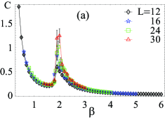
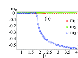
Figure 1: (a) Specific heat for $(c_{2},c_{4},c_{5})=(0.5,4.0,1.0)$ and $c_{1}=c_{3}=0$. At $\beta\simeq 2.0$, $C$ exhibits a sharp peak indicating a second-order FM phase transition. (b) Each component of magnetization $m_{\mu}$ vs $\beta$. For $T<T_{\rm FM}$, $m_{3}$ develops, whereas $m_{1}$ and $m_{2}$ are zero within the errors as expected.

We first show that the model (2.21) exhibits a FM phase transition as $T$ is lowered. To this end, we put $c_{1}=c_{3}=0$ and $(c_{2},c_{4},c_{5})=(0.5,4.0,1.0)$, and increase $\beta$ in the Boltzmann factor of Eq.(2.21). In Fig.1 we show $C$ and $m_{\mu}$. It is obvious that a second-order phase transition to the FM state takes place at $\beta_{\rm FM}=1/T_{\rm FM}\simeq 2.0$. We verified that other cases with various values of $c_{2,4,5}$ exhibit similar FM phase transitions.

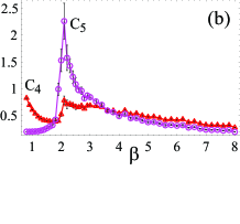
Figure 2: (a) Specific heat vs $\beta$ for $(c_{1},c_{3})=(0.2,0.2)$ and $(c_{2},c_{4},c_{5})=(0.5,4.0,1.0)$ ($L=20$). There are a large peak at $\beta\simeq 2.1$ and a small one at $\beta\simeq 4.5$. (b,c) Specific heat $C_{i}$ of each term of $F$ in (2.21) vs $\beta$. The small and broad peak at $\beta\simeq 4.5$ in $C$ is related to fluctuations of $c_{1}$-term.

Next, let us study the SC phase transition. Here it is useful to consider the case of all $c_{i}=0$ except for $c_{1}$. Then the model is related to the CP¹+U(1) lattice gauge theorytakashima which has the energy of the form $f_{r}=-(c_{1}/2)\sum(\bar{z}Uz+{\rm c.c.})+F_{A}$ where $F_{A}$ is the compact version (2.5). In fact, they agree by setting $1/e^{2}=0$. The phase structure of this model is studied in Ref.takashima and it is found that the phase transition from the confinment phase to the Higgs phase takes place at $c_{1}\simeq 2.85$ for $1/e^{2}=0$. Thus the SC state exists at sufficiently large $c_{1}$.

For simulation, we put $(c_{1},c_{3})=(0.2,0.2)$ and $(c_{2},c_{4},c_{5})=(0.5,4.0,1.0)$. In Fig.2a, we show $C$ vs $\beta$. There are a large and sharp peak at $\beta\simeq 2.1$ and a small and broad one at $\beta\simeq 4.5$. In order to understand physical meaning of the second peak, it is useful to measure “specific heat” of each term $f_{i}$ in the free energy (2.16) defined by $C_{i}=\langle(F^{\prime}_{i}-\langle F^{\prime}_{i}\rangle)^{2}\rangle/L^{3}$. Fig.2c shows that the specific heat of the $c_{1}$-term has a relatively large and broad peak at $\beta\simeq 4.5$. Then we conclude that the SC phase transition takes place at $\beta_{\rm SC}\simeq 4.5$.

To verify this conclusion, we show $G_{m}(r)$ and $G_{S}(r)$ in Fig.3. At $\beta=2.5$, $G_{m}(r)$ exhibits a finite amount of the FM order, whereas $G_{S}(r)$ decreases very rapidly to vanish. This means that, as $T$ is decreased, the FM transition takes place first and then the SC transition does. Therefore, for $\beta\geq\beta_{\rm SC}\simeq 4.5$, the FM and SC orders coexist.

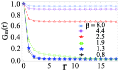
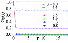
Figure 3: Correlation functions $G_{m}(r)$ and $G_{S}(r)$ at various $T$’s for $L=20$. $c_{i}$’s are the same as in Fig.2.

It is interesting to clarify the relation between the bare transition temperature $T^{0}_{\rm SC}$ in Eq.(2.11) and the genuine transition temperature $T_{\rm SC}$. From Eq.(2.21), any physical quantity is a function of $\beta c_{i}$. In the numerical simulations, we fix the values of $c_{i}$ and vary $\beta$ as explained. Then the result $\beta_{\rm SC}\simeq 4.5$ means

$$\beta c_{1}|_{T=T_{\rm SC}}=4.5\times 0.2.$$ (3.5)

By using Eq.(2.20), this gives the following relation;

$${1\over T_{\rm SC}}{K\alpha(T^{0}_{\rm SC}-T_{\rm SC})a\over\lambda}=0.90,$$

$$T_{\rm SC}=\Big{(}1+{0.90\ \lambda\over K\alpha\ a}\Big{)}^{-1}T^{0}_{\rm SC}.$$ (3.6)

Eq.(3.6) shows that the transition temperature is lowered by the fluctuations of the phase degrees of freedom of Cooper pairs. We expect that a relevant contribution to lowering the SC transition temperature comes from vortices that are generated spontaneously in the FMSC as we show in Sec.III.B.

After having confirmed that the genuine critical temperature can be calculated by the critical value of $\beta$ with fixed $c_{i}$, we use the word temperature in the rest of the paper just as the one defined by $T\equiv 1/\beta$ while $c_{i}$ are $T$-independent parameters.

Figure 4: Gauge-boson mass $M_{\rm G}$ of the external magnetic field propagating in $x$-$y$ plane vs $\beta$ for the same $c_{i}$ as in Fig.2 and ${c_{2}}^{\prime}=3.0$ ($L=16$). At the SC phase transition point $\beta_{\rm SC}\simeq 4.5$ (indicated by an arrow) determined by the peak of $C$, $M_{\rm G}$ starts to increase from small values.

Meissner effect is one of the most important phenomena for a SC order. To study it, we follow the following stepstakashima ; (i) introduce a vector potential $A^{\rm ex}_{x\mu}$ for an external magnetic field, (ii) couple it to Cooper pairs by replacing $U_{x\mu}\to U_{x\mu}\exp(iA^{\rm ex}_{x\mu})$ in the $c_{1}$ term of $f_{x}$ and add its magnetic term $f^{\rm ex}_{x}=+{c_{2}}^{\prime}(\vec{m}_{x}^{\rm ex})^{2}\ (c_{2}^{\prime}>0)$ to $f_{x}$ with $\vec{m}^{\rm ex}_{r}$ defined in the same way as (2.17) by using $A^{\rm ex}_{x\mu}$, (iii) let $A^{\rm ex}_{x\mu}$ fluctuate together with $z_{xa}$ and $A_{x\mu}$ and measure an effective mass $M_{\rm G}$ of $A^{\rm ex}_{x\mu}$ via the decay of correlation functions of $\vec{m}_{x}^{\rm ex}$. The result of $\vec{m}^{\rm ex}_{x}$ propagating in the 1-2 plane is shown in Fig.4. It is obvious that the mass $M_{\rm G}$ starts to develop at the SC phase transition point, and we conclude that Meissner effect takes place in the SC state.

III.2 SC transition and vortices in a constant magnetic field

Because the observed SC state in Figs.2 and 3 coexists with the FM order, it is expected that vortices of the SC order parameter are induced there spontaneoulyvortex . To verify this expectation, we set the vector potential $A_{x\mu}$ to a position-dependent but nonfluctuating value that corresponds to a uniform magnetic field in the third-direction, and study the behavior of $z_{xa}$ itself. In this case, the free energy $f_{x}$ loses the local gauge symmetry (2.19), and therefore the correlation function of $z_{xa}$,

$$G_{z}(x-x_{0})=\langle\bar{z}_{x}\cdot z_{x_{0}}\rangle,$$ (3.7)

has nonvanishing values in the SC phase.

In Fig.5, we show $C$ and $G_{z}(x)$ for two cases of fixed $\vec{m}_{x}$. For the case with $\vec{m}_{x}=(0,0,{\pi\over 4})^{\rm t}$, $C$ has a shape similar to $C_{1}$ in Fig.2c, and indicates a SC phase transition at $\beta\simeq 4.8$. $G_{z}(r)$ exhibits fluctuating behavior even for low $T$’s, $\beta\geq 4.9$. This suggests that vortices are spontaneouly generated in the SC state violating spatial unifomity, and their locations fluctuate. In the other case of $\vec{m}_{x}=(0,0,\pi)^{\rm t}$, $C$ has a sharper peak at $\beta\simeq 4.5$, and $G_{z}(r)$ exhibits clear periodically oscillating behavior with the period $4\times$(lattice spacing). This implies that, in this case, locations of vortices are rather stable compared with the case of $m_{x3}={\pi\over 4}$.

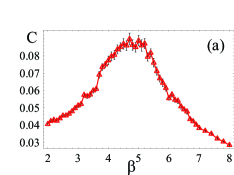
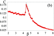
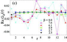
Figure 5: The results for a constant magnetic field $\vec{m}_{x}=(0,0,m_{x3})^{\rm t}$ at $c_{1}=c_{3}=0.2$ ($L=16$). (a,b) Specific heat $C$ and (c,d) the real part of SC correlation function $G_{z}(r)$ in the 1-2 plane. (a,c) $m_{x3}=\pi/4$ and (b,d) $m_{x3}=\pi$.

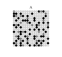
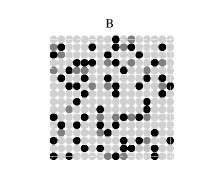
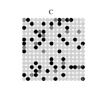
$V_{x}^{\pm}$

Figure 6: Snapshots of vortex densities $V_{x}^{\pm}$ at $c_{1}=c_{3}=0.2$ for a fixed $\vec{m}=(0,0,\pi/4)\ (L=16)$. Black dots; $V_{x}^{\pm}$= 0.875, Dark gray dots; -1.125, Light gray dots; -0.125. (A)$V_{x}^{+}$ at $\beta=3.0$, (B)$V_{x}^{-}$ at $\beta=3.0$, (C)$V_{x}^{+}$ at $\beta=7.0$, (D)$V_{x}^{-}$ at $\beta=7.0$. The average magnitude $\langle|V_{x\pm}|\rangle$ is (A) 0.387, (B) 0.380, (C) 0.331 and (D) 0.335. The points $V_{x}^{\pm}=-0.125=-m_{3}/(2\pi)$ reflect $\vec{m}$ itself.

In order to verify the above expectation, we calculate vortex density directly. In the present model, one may define the following two kinds of gauge-invariant vortex densities $V_{x}^{+}$ and $V_{x}^{-}$ in the 1-2 plane;

$$z_{x}^{\pm} \equiv z_{x1}\pm iz_{x2}\equiv\rho_{x}^{\pm}\exp(i\theta_{x}^{\pm}),$$

$$V_{x}^{\pm} \equiv \frac{1}{2\pi}[{\rm mod}(\theta_{x+1}^{\pm}-\theta_{x}^{\pm}-A_{x1})$$ (3.8)

$$+{\rm mod}(\theta_{x+1+2}^{\pm}-\theta_{x+1}^{\pm}-A_{x+1,2})$$

$$-{\rm mod}(\theta_{x+1+2}^{\pm}-\theta_{x+2}^{\pm}-A_{x+2,1})$$

$$-{\rm mod}(\theta_{x+2}^{\pm}-\theta_{x}^{\pm}-A_{x2})],$$

where mod$(x)\equiv$ mod$(x,2\pi)$. In short, $V_{x}^{\pm}$ describes vortices of electron pairs with the amplitude $\psi_{\uparrow\uparrow({\downarrow\downarrow})}=\psi_{1}\pm i\psi_{2}\propto z_{1}\pm iz_{2}$.

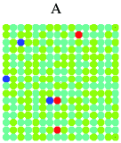
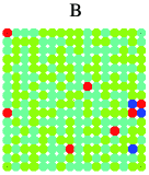
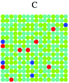
$V_{x}^{\pm}$

Figure 7: Snapshots of vortex densities $V_{x}^{\pm}$ at $c_{1}=c_{3}=0.2$ for a fixed $\vec{m}=(0,0,\pi)\ (L=16)$. (A)$V_{x}^{+}$ at $\beta=3.0$, (B)$V_{x}^{-}$ at $\beta=3.0$, (C)$V_{x}^{+}$ at $\beta=7.0$, (D)$V_{x}^{-}$ at $\beta=7.0$. The average magnitude $\langle|V_{x}^{\pm}|\rangle$ is (A) 0.528, (B) 0.537, (C) 0.560 and (D) 0.508. The points $V_{x}^{\pm}=-0.5=-m_{3}/(2\pi)$ reflect $\vec{m}$ itself.

In Fig.6 we present snapshots of $V_{x}^{\pm}$ at $c_{1}=c_{3}=0.2$ for fixed values of gauge potential $A_{x\mu}$ corresponding to a constant magnetization, $\vec{m}=(0,0,\frac{\pi}{4})^{\rm t}$. It shows that (i) both of the fluctuations around zero, $\langle|V_{x}^{\pm}|\rangle$, decrease as $\beta$ increases, and (ii) $V_{x}^{+}$ has larger fluctuations than $V_{x}^{-}$ at high $T$, whereas smaller ones at low $T$. These behaviors are consistent with the Zeeman $c_{3}$-term in the energy $f_{x}$ of (2.16), which distinguishes the $z_{x}^{+}$ order and the $z_{x}^{-}$ order, and the fact that $\vec{m}$ directs to the third-direction in the present case. In Fig.7, we also show the vortex snapshots at $c_{1}=c_{3}=0.2$ and $\vec{m}=(0,0,\pi)^{\rm t}$. Compared with the case $\vec{m}=(0,0,\frac{\pi}{4})^{\rm t}$, vortices here are located rather systematically as we expected from the result of correlation function $G_{z}(r)$.

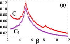
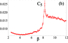
Figure 8: Specific heats for $c_{5}=0.4\ (L=12)$. (a) Total $C$ and the specific heat $C_{1}$ of the $c_{1}$-term, (b) $C_{5}$ of the $c_{5}$-term. Order of two phase transitions is interchanged ($\beta_{\rm SC}<\beta_{\rm FM}$).

III.3 Order of FM and SC phase transitions and phase diagram

Let us next examine the possibility that the order of the FM and SC phase transitions are interchanged as the value of $c_{5}$ is decreased. As the $c_{5}$-term in $f_{x}$ tends to align $\vec{m}_{x}$, $T_{\rm FM}$ decreases as $c_{5}$ is decreased. Most of the FMSC materials loses the FM order as the applied $P$ is increased, and then it is phenomenologically expected that $c_{5}$ is a decreasing function of $P$. We consider several cases with $c_{5}=1.5,1.0,0.7,0.5,0.4$ and $0.3$, while other $c_{i}$ are fixed to the same values as those in Fig.2 where $c_{5}=1.0$.

We find that the order of two phase transitions actually interchanges at $c_{5}\simeq 0.5$. In Fig.8, we show the specific heat $C,C_{1},C_{5}$ for $c_{5}=0.4$. $C$ has the two peaks at $\beta_{\rm SC}\sim 5.0<\beta_{\rm FM}\sim 8.3$. $C_{1}$ is sharper than in the case of $c_{5}=1.0$ in Fig.2.

In Fig.9 we present $G_{m}(r)$ and $G_{S}(r)$ with $r$ in the 1-2 plane for $c_{5}=0.4$, which exhibit very peculiar behavior; In the FM and SC coexisting phase ($T<T_{\rm FM}$), they have nonvanishing values only near the surface of the lattice in contrast with Fig.3. This behavior survives in larger systems. For example, we define the thickness $\Delta L$ of the coexisting region such that the ordered region in the 1-2 plane occupies the interval $2+\Delta L+({\rm disordered\ region})+\Delta L+2$ in the lattice length $2+L+2$ in the $\mu=1,2$ directions. We obtain $\Delta L\simeq 3$ for $L=12$(Fig.9) and $\Delta L\simeq 4$ for $L=16$, so about the outer half region in the linear dimension is occupied by the ordered state. This implies that the FMSC coexisting phase appear in the region including the surface of the material, and not in the central region inside the system. We note that this “surface” region is not two-dimensional but 3D, because the SC-FM transition is a genuine second-order one, which is not allowed in a two-dimensional systemmermin . This phenomenon is a prediction of the present model.

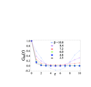
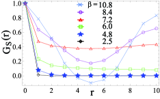
Figure 9: Correlation functions $G_{m}(r)$ and $G_{S}(r)$ at $c_{5}=0.4$ ($L=12$). The other $c_{i}$ are the same as those in Fig.2. They exhibit orders near the surface of the lattice.

It is intriguing to draw a phase diagram in the $P$-$T$ plane assuming certain phenomenological relation between $c_{5}$ and $P$. In the experiments, the critical temperature $T_{\rm FM}$ is a decreasing function of $P$. This means that the parameters $c_{2},\ c_{4}$ and $c_{5}$ in Eq.(2.16) vary as functions of $P$. Changes of $c_{2}$ and/or $c_{4}$ influence the magnitude of the magnetization vector $\vec{m}_{x}$ and result in a change of $c_{5}$ after a renormalization of $\vec{m}_{x}$. Then for example, one may “phenomenologically” assume

$$c_{5}=c^{\star}_{5}\Big{(}1-{P(c_{5})\over P_{\rm c}}\Big{)}^{1/\gamma},$$ (3.9)

where $P_{\rm c}$ is the critical pressure at which the FM order disappears even at $T\rightarrow 0$ (i.e., at $c_{5}=0$), $c_{5}^{\star}$ is the value of $c_{5}$ at which $P=0$, and the power $\gamma$ is a fitting parameter. In Fig.10 we show the phase diagram drawn with certain choice of these parameters.This phase diagram has a similar structure to the experimental result of UCoGe.

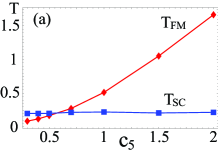
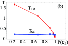
Figure 10: Phase diagrams in (a) $c_{5}$-$T$ and (b) $P$-$T$ planes with $P_{\rm c}=1.0$, $c_{5}^{\star}=2.2$ and $\gamma=3.0$. $c_{1}-c_{4}$ are same as in Fig.2.

In the same way as decreasing $c_{5}$, the case of increasing $c_{3}$ has been studied with several choices of $c_{5}$ and $(c_{1},c_{2},c_{4})=(0.2,0.5,4.0)$. Both $T_{\rm FM}$ and $T_{\rm SC}$ increase as $c_{3}$ increases. Furthermore, for sufficiently large values such as $c_{3}=1.5$, $T_{\rm FM}>T_{\rm SC}$ even for $c_{5}=0.5$ as expected. This indicates that the present model with larger $c_{3}$ may provide a phase diagram similar to that of UGe₂ and URhGe.

IV Conclusion

In summary, we have proposed a GL model defined on the 3D lattice for the FMSC state, and shown that it explains some experimental observations such as the

phase diagram and the homogeneous and inhomogeneous FMSC states. This model naturally includes effects of topological excitations, vortices, that play an important role for the SC phase transition in the FM state. Although the obtained global phase structure is similar to that of MFT, the appearance of inhomogeneous configurations such as the FMSC state and vortex configurations are certainly beyond the scope of MFT. In the present analysis, we consider the “London limit”, in which the radial fluctuations of the two-gap SC order parameters are ignored. As we explained in Sec.II.A., these fluctuations may change the order of SC phase transitions and may play an important role in SC transitions that are induced by an external magnetic-field. This problem is under study and results will be reported in a future publication.

- (1) S. S. Saxena1, P. Agarwal, K. Ahilan, F. M. Grosche, R. K. W. Haselwimmer, M. J. Steiner, E. Pugh, I. R. Walker, S. R. Julian, P. Monthoux, G. G. Lonzarich, A. Huxley, I. Sheikin, D. Braithwaite and J. Flouquet, Nature (London) 406, 587 (2000); A. Huxley, I. Sheikin, E. Ressouche, N. Kernavanois, D. Braithwaite, R. Calemczuk and J. Flouquet, Phys. Rev. B 63, 144519 (2001); N. Tateiwa, T. C. Kobayashi, K. Hanazono, K. Amaya, Y. Haga, R. Settai and Y. Onuki, J. Phys. Condens. Matter 13, L17 (2001).
- (2) D. Aoki, A. Huxley, E. Ressouche, D. Braithwaite, J. Floquet, J.-P. Brison, E. Lhotel and C. Paulsen, Nature (London) 413, 613 (2001).
- (3) N. T. Huy, A. Gasparini, D. E. de Nijs, Y. Huang, J. C. P. Klaasse, T. Gortenmulder, A. de Visser, A. Hamann, T. Görlach and H. v. Löhneysen, Phys. Rev. Lett. 99, 067006 (2007).
- (4) E. Slooten, T. Naka, A. Gasparini, Y. K. Huang and A. de Visser, Phys. Rev. Lett. 103, 097003 (2009).
- (5) K. Machida and T. Ohmi, Phys. Rev. Lett. 86, 850 (2001), M. B. Walker and K. V. Samokhin, Phys. Rev. Lett. 88, 207001 (2002).
- (6) V. P. Mineev, Phys. Rev. B 66, 134504 (2002).
- (7) For experimental evidence, see F. Hardy and A. D. Huxley, Phys. Rev. Lett. 94, 247006 (2005); A. Harada, S. Kawasaki, H. Mukuda, Y. Kitaoka, Y. Haga, E. Yamamoto, Y. Onuki, K. M. Itoh, E. E. Haller and H. Harima, Phys. Rev. B 75, 140502 (2007).
- (8) The preliminary version of the present work has been reported in 26th Int. Conf. on Low Temp. Phys., Beijing, Aug. 10-17 (2011), A. Shimizu, H. Ozawa, I. Ichinose and T. Matsui, J. Phys. (Conference Series) in press.
- (9) V. P. Mineev and T. Champel, Phys. Rev. B 69, 144521 (2004); D. V. Shopova and D. I. Uzunov, Phys. Rev. B 79, 064501 (2009); X. Jian, J. Zhang and Q. Gu, Phys. Rev. B80, 224514 (2009).
- (10) S. Coleman and E. Weinberg, Phys. Rev. D7, 1888 (1973).
- (11) K. Kajantie, M. Karjalainen, M. Laine and J. Peisa, Phys. Rev. B57, 3011 (1998) and references cited therein.
- (12) K. Kajantiea, M. Laineb, T. Neuhausc, A. Rajantied and K. Rummukainene Nucl. Phys. Proc. Suppl. 106, 959 (2002).
- (13) M. Chavel, Phys. Lett. B 378, 227 (1996).
- (14) M. B. Einhorn and R. Savit, Phys. Rev. D 17, (1978) 2583; D 19, (1979) 1198.
- (15) K. G. Wilson, Phys. Rev. D 10, (1974) 2445, A. M. Polyakov, Phys. Lett. 59B 82 (1975).
- (16) S. Wenzel, E. Bittner, W. Janke, A. M. J. Schakel, A. Schiller, Phys. Rev. Lett. 95, 051601 (2005).
- (17) D. J. E. Callaway and L. J. Carson, Phys. Rev. D 25, 531 (1981).
- (18) T. Ono, S. Doi, Y. Hori, I. Ichinose and T. Matsui, Ann. Phys. 324, 2453 (2009).
- (19) E. Smørgrav, J. Smiseth, E. Babaev and A. Sudbø, Phys. Rev. Lett. 94, 096401 (2005), and references cited therein.
- (20) N. T. Huy, D. E. de Nijs, Y. K. Huang and A. de Visser, Phys. Rev. Lett. 100, 077002 (2008).
- (21) We have included the charge in .
- (22) See, e.g., J.Zinn-Justin, “Quantum field theory and critical phenomena”, (1993, Clarendon press, Oxford).
- (23) S. Takashima, I. Ichinose and T. Matsui, Phys. Rev. B 72, 075112 (2005).
- (24) T. Ohta, T. Hattori, K. Ishida, Y. Nakai, E. Osaki, K. Deguchi, N. K. Sato and I. Satoh, J. Phys. Soc. Jpn. 79, 023707 (2010); K. Deguchi, E. Osaki, S. Ban, N. Tamura, Y. Simura, T. Sakakibara, I. Satoh and N. K. Sato, J. Phys. Soc. Jpn. 79, 083708 (2010).
- (25) N. D. Mermin and H. Wagner, Phys. Rev. Lett. 17, 1133 (1966), P. C. Hohenberg, Phys. Rev. 158, 383 (1967), S. Coleman, Commun. Math. Phys. 31, 259 (1973).
- (26) E. A. Yelland, S. J. C. Yates, O. Taylor, A. Griffiths, S. M. Hayden and A. Carrington, Phys. Rev. B 72, 184436 (2005); E. A. Yelland, S. M. Hayden, S. J. C. Yates, C. Pfleiderer, M. Uhlarz, R. Vollmer, H. v. Löhneysen, N. R. Bernhoeft, R. P. Smith, S. S. Saxena and N. Kimura, Phys. Rev. B 72, 214523 (2005).