Stretched exponential behavior and random walks on diluted hypercubic lattices

Abstract

Diffusion on a diluted hypercube has been proposed as a model for glassy relaxation and is an example of the more general class of stochastic processes on graphs. In this article we determine numerically through large scale simulations the eigenvalue spectra for this stochastic process and calculate explicitly the time evolution for the autocorrelation function and for the return probability, all at criticality, with hypercube dimensions $N$ up to $N=28$. We show that at long times both relaxation functions can be described by stretched exponentials with exponent $1/3$ and a characteristic relaxation time which grows exponentially with dimension $N$. The numerical eigenvalue spectra are consistent with analytic predictions for a generic sparse network model.

Introduction

In 1854 R. Kohlrausch used a phenomenological expression

$$q_{K}(t)=\exp(-(t/\tau)^{\beta})$$ (1)

to parametrize the non-exponential decay of the electric polarization of Leyden jars (primitive capacitors)RK ; his son F. Kohlrausch later used the same expression to analyse creep in galvanometer suspensions FK . A century later, in 1951 Weibull introduced weibull the closely related Weibull function; this survival probability function eliazar which is widely used in the engineering literature is strictly of the Kohlrausch form, Eqn. (1). In 1970 Williams and Watts re-discovered the Kohlrausch function in the context of dielectric relaxationWW . Under the name of “stretched exponential” chamberlin the KWW (Kohlrausch-Williams-Watts) function has become ubiquitous in phenomenological analyses of non-exponential relaxation data, experimental or numerical. In particular the KWW form was used by Ogielski in a phenomenological fit the decay of the autocorrelation function at equilibrium for a $3d$ Ising spin glass model ogi1985 .

Many arguments have been given as to why under certain assumptions, specific systems should show KWW relaxation phil ; havl ; rasa ; dons1 ; dons2 ; gras ; gotz ; ian1 ; ian2 ; ian3 , but there have always been lingering suspicions that for most cases the KWW expression is nothing more than a convenient fitting function of no fundamental significance.

It was conjectured ian1 that KWW relaxation is the signature of a complex configuration space. Thus from the argument which follows it was suggested that random walks on a diluted hypercube (a hypercube with a fraction $p$ of vertices occupied at random) near the critical concentration for percolation $p_{c}$ erdos1979 would lead to an autocorrelation function decay of the form $q(t)\sim\exp[-(t/\tau)^{\beta}]$, with a specific value of the exponent, $\beta=1/3$.

For random walks at percolation threshold in a randomly occupied Euclidean (flat) space of dimension $d$ such as $\mathbb{Z}^{d}$, the familiar Fickian diffusion law $\langle R^{2}\rangle\sim t$ is replaced by a sub-linear diffusion $\langle R^{2}\rangle\sim t^{\beta_{d}}$, with $\beta_{d}\equiv 1/3$ for $d\geq 6$ alexander:82 . Random walks on the surface of a full [hyper]sphere $\mathbb{S}_{d-1}$ in any dimension $d$ are characterized by the generic law $\langle\cos(\theta)\rangle=\exp(-(t/\tau))$ where $\theta$ denotes the generalized angular displacement of the walker debye ; caillol . It was argued ian1 that random walks on percolation clusters at threshold inscribed on [hyper]spheres would be characterized by relaxation of the form $\langle\cos(\theta)\rangle=\exp(-(t/\tau)^{\beta_{d}})$ with the same exponents $\beta_{d}$ as in the corresponding Euclidean space. This was demonstrated numerically for $d=3$ to $8$ jund . A hypercube being topologically equivalent to a hypersphere, for random walks on a diluted hypercube at threshold one then expects stretched exponential relaxation with exponent $\beta=1/3$.

The diluted hypercube at threshold can alternatively be considered as a specific example of a sparse graph. Remarkably, analytic expressions for diffusion on general sparse graphs bray1988 ; samukhin2008 derived from a quite different line of argument also lead to stretched exponential relaxation expressions with the same specific value $\beta=1/3$ for the exponent.

Here we present numerical data for random walks on the diluted hypercube at threshold up to dimension $N=28$ which are consistent with these conclusions. We argue that the KWW relaxation observed phenomenologically in numerous complex systems just above their respective critical temperatures is not an artifact, but is the signature of a universal form of coarse grained configuration space morphology which precedes a glass transition.

Laplace transforms and random networks

Quite generally, any relaxation function $q(t)$ can equivalently be characterized by its Laplacian, a relaxation mode density (or eigenvalue density) function $\rho(s)$ defined by:

$$q(t)\equiv\int_{0}^{\infty}\rho(s)e^{-st}ds$$ (2)

with the normalization condition

$$\int_{0}^{\infty}\rho(s)ds=1$$ (3)

In model systems it can be possible to establish analytically or numerically the distribution $\rho(s)$ which can then be inverted to obtain $q(t)$. The inverse Laplace transform of a numerical or experimental $q_{K}(t)$ to obtain $\rho(s)$ is much more difficult unless $q(t)$ is known to very high precision over a wide range of $t$. This is an ill-conditioned problem as different $\rho(s)$ distributions can lead to almost indistinguishable $q(t)$.

Pollard pollard (see Berberan-Santos berberan2008 ) provided an exact inversion of the pure stretched exponential relaxation function $q_{K}(t)$ 1 :

$$\rho_{K,\beta}(s)=\frac{\tau}{\pi}\int_{0}^{\infty}\exp\left[-u^{\beta}\cos\left(\frac{\beta\pi}{2}\right)\right]\cos\left[u^{\beta}\sin\left(\frac{\beta\pi}{2}\right)\right]\cos(s\tau u)\;du$$ (4)

For $\beta<1$, $\rho_{K,\beta}(s)$ can be expressed in terms of elementary functions only for $\beta=1/2$ pollard ; in that case

$$\rho_{K,1/2}(s)=[\tau/2\pi^{1/2}(s\tau)^{3/2}]\exp(-1/4s\tau)]$$ (5)

To a good approximation, for general $\beta$ the large $s$ (short time) limit takes the form $\rho_{K,\beta}\sim s^{-(1+\beta)}$ and the small $s$ (long time) limit the form $\rho_{K,\beta}\sim(s)\exp[s^{-\beta/(1-\beta)}]$.

It should be kept in mind that at short times observed relaxation functions usually deviate from the “asymptotic” form. Also at very long times for finite sized systems the relaxation is controlled by the smallest non-zero value of $s$, $s_{1}$. For time $t>s_{1}^{-1}$ the relaxation will tend to a pure exponential, $q(t)\sim\exp[-ts_{1}]$, but for large systems this condition corresponds to extremely long times and we will not consider it. What we are interested in is to establish the form of the relaxation in the regime where the mode distribution is no longer affected by short time effects and where $\rho(s)$ can be considered continuous.

Random networks

Random walks on the diluted $N$-simplex or hypertetrahedron which is an Erdös-Rényi graph having dead ends and vertices with two connections, was studied theoretically by Bray and Rodgers bray1988 using Replica theory. They showed that in this model the return function $p_{ret}(t)$, the probability that the walker will have returned to the origin after $t$ steps, behaves like a stretched exponential with exponent $1/3$.

Samukhin et al samukhin2008 have made analytic studies of random walks and relaxation processes on uncorrelated Random Networks. They considered a stochastic process governed by the Laplacian operator occurring on a random graph with $N^{*}$ nodes, taking the limit as $N^{*}\to\infty$. They find that the determining parameter in this problem is the minimum degree $q_{m}$ of vertices (i.e. the minimum number of neighbors to any given vertex). For $q_{m}=2$, meaning that the network is “sparse”, the graph tends to a random Bethe lattice in which almost all finite subgraphs are trees, i.e., they contain almost no closed loops. In the present context the essential statement of Samukhin et al samukhin2008 is that when $q_{m}=2$ the mode density function $\rho_{S}(s)$ for this very general model can be approximated by

$$\rho_{S}(s)=s^{-4/3}\exp(-a/\sqrt{s})$$ (6)

where

$$a=\sqrt{\frac{4\tau^{-}1}{3}}$$ (7)

with a similar expression for $q_{m}=1$ (graphs with dead ends). Then for a graph with $N^{*}$ vertices the asymptotics at $t>\ln N^{*}$ for the probability of return to the starting point at time $t$ during a random walk on the network (the ”autocorrelator” samukhin2008 ) will be

$$p_{ret,S}(t)\sim t^{\eta}\exp[-3(a/2)^{2/3}t^{1/3}],$$ (8)

a stretched exponential having exponent $1/3$, multiplied by a mildly time dependent prefactor ($\eta$ is small). This limit should be observable if the network size satisfies $(\ln N^{*})^{2/3}\gg 1$.

I Hypercube model

We have already addressed the hypercube problem numerically through Monte Carlo techniques lemke1996 and through the explicit solution of Master equations lemke2000 ; almeida2000 . In this paper we extend these results by investigating the time evolution for the autocorrelation function $q(N,t)$, the return probability $p_{ret}(N,t)$, and the eigenvalue spectrum $\rho(N,s)$ for diffusion on diluted hypercubes of dimension $N$ near the critical occupation probability $p_{c}(N)$, for $N$ up to $28$.

Consider a hypercube (or n-cube) in [high] dimension $N$, $\mathbb{Q}_{N}$, with a fraction $p$ of its $2^{N}$ vertices occupied at random. It is well established erdos1979 ; bollobas ; borgs that there is a critical threshold at $p_{c}(N)\sim 1/N$. For $p>p_{c}(N)$ the occupied vertices having one or more occupied vertices as neighbors make up a giant spanning cluster; for $p<p_{c}$ there exist only small clusters (each with less than $N$ elements). By analogy with the equivalent situation in randomly occupied Euclidean space we will refer to $p_{c}$ as the “percolation” threshold.

Gaunt and Brak gaunt1984 predict that the dependency of the critical site percolation concentration $p_{c}$ on a hypercubic lattice of dimension $d$, $\mathbb{Z}^{d}$, or on a hypercube of dimension $N$, $\mathbb{Q}_{N}$, is given to order $4$ by:

$$p_{c}(\sigma)=\sigma+\frac{3}{2}\sigma^{2}+\frac{15}{14}\sigma^{3}+\frac{83}{4}\sigma^{4}\ldots$$ (9)

where $\sigma(d)=1/(2d-1)$ for the hypercubic lattice and $\sigma(N)=1/(N-1)$ for the hypercube gaunt1976 . Although the terms in this expression are expected to be exact, the demonstration is not entirely rigorous gaunt1984 , and the series is obviously truncated. Grassberger grassberger2003 tested the equation (9) through large scale Monte Carlo simulations on $\mathbb{Z}^{d}$ and verified that for $d>10$ it represents the numerically determined $p_{c}(d)$ to within a small correction term. We will work with samples having vertex concentrations $p(N)$ equal to the values $p_{c}(N)$ given by the truncated series equation (9). For different samples $k$ the individual critical values $p_{c}(k)$ will in fact be distributed about the average value borgs .

For $p>p_{c}(N)$ we can define a random walk along edges on the giant cluster. Start at any vertex $i$ on the giant cluster. Choose at random a vertex $j$ on the hypercube, near neighbor to $i$. If the vertex $j$ is also on the giant cluster and so accessible, move to $j$; otherwise the walker remains one time step longer at the vertex $i$. This evolution rule is chosen to mimic Monte Carlo simulations using Metropolis dynamics.

We can compare the autocorrelation function $q(N,t)$ obtained from this procedure, ($q(N,t)$ is defined in Eq. (16) below), to the time dependent autocorrelation $\langle S_{i}(t).S_{i}(0)\rangle$ measured in thermodynamic models for systems of Ising spins $S_{i}$ ogi1985 and even to experimental magnetization decay results. From a theoretical point of view it is often more convenient to investigate the “return probability” $p_{ret}(t)$ that is basically the probability of finding the walker at the origin of the system after $t$ steps ($p_{ret}(N,t)$ is defined in Eq. (18) below). For any network $p_{ret}(t)$ can be defined, while $q(t)$ can be defined conveniently only on models such as the hypercube which have a suitable metric.

The numerical data near criticality show that the long time relaxations of the autocorrelation parameter $q(N,t)$ and of the return probability $p_{ret}(N,t)$ are consistent with stretched exponentials having an exponent $\beta=1/3$ over many orders of magnitude in time.

Algorithm

The time evolution of the entire probability distribution for the walker after $t$ steps, $\vec{\Pi}(t)$, can be described by a Master Equation. At $t=0$ the walker is localized on a single vertex $i_{o}$ on the hypercube; the probability distribution then diffuses over the system at each time step following the equation:

$$\Pi_{i}(t)=\Pi_{i}(t-1)+\left[\sum_{j}\Pi_{i}(t-1)W(j\to i)-\Pi_{j}(t-1)W(i\to j)\right]$$ (10)

where $W(i\to j)$ represents the transition probability that is given by:

$$W(i\to j)=\left\{\begin{array}[]{l l}\frac{1}{N}&\mbox{if $i$ vertex and $j$ vertex are allowed}\\ 0&\mbox{otherwise}\end{array}\right.$$ (11)

The equation (10) can be rephrased as:

$$\vec{\Pi}(t)=F\vec{\Pi}(t-1)$$ (12)

where $F$ is the linear evolution operator.

Since this process is Markovian we can diagonalize $F$; the smallest eigenvalue corresponding to the infinite time equilibrium limit (where all sites become equally populated) is 1. We can determine $U$ and $D$ satisfying:

$$F=U^{T}DU$$ (13)

where $D$ is a diagonal matrix. For practical reasons it is convenient to diagonalize $F$ so as to investigate the temporal evolution of the relevant quantities. We use:

$$\Pi(t)=F^{t}\Pi(0)=U^{T}D^{t}U\Pi(0)$$ (14)

We choose the initial condition as:

$$\Pi_{i}(0)=\delta_{ii_{o}}$$ (15)

where $i_{o}$ is a vertex on the giant cluster.

The value of the normalized autocorrelation function $q(t)$ after time $t$ for a given walk starting from $i_{o}$ and arriving at $i$ after time $t$ can be defined by:

$$q(t)=\left\langle\frac{1}{N_{G}}\sum_{i_{o}}\sum_{i}\Pi_{i}(t)\frac{N-2d_{H}(i,i_{o})}{N}-q_{\infty}\right\rangle$$ (16)

where $d_{H}(i,i_{o})$ is the Hamming distance between vertex $i$ and the initial state, $N_{G}$ is the number of vertices on the giant cluster, $q_{t=\infty}$ for a given realization is given by:

$$q_{t=\infty}=\frac{1}{N_{G}^{2}}\sum_{ii_{o}}\frac{N-2d_{H}(i,i_{o})}{N}$$ (17)

and the averages are over different realizations of the diluted hypercube.

We also calculated $p_{ret}$ defined by:

$$p_{ret}(t)=\left\langle\frac{1}{N_{G}}\sum_{i_{o}}\Pi_{i_{o}}(t)-\frac{1}{N_{G}}\right\rangle$$ (18)

We can show that:

$$p_{ret}(t)=\frac{1}{N_{G}}\left\langle\sum_{j}\lambda_{j}^{t}-\frac{1}{N_{G}}\right\rangle$$ (19)

This quantity is easier to calculate theoretically than $q(t)$, but it is not useful to compare with results on model spin systems or experiments. We can write this equation in a more convenient form:

$$p_{ret}(t)=\frac{1}{N_{G}}\left\langle\sum^{\prime}_{s\neq 0}e^{-s_{i}t}\right\rangle$$ (20)

where $s=-\ln\lambda$ and we excluded $\lambda=1$ eigenvalue. Another convenient form for investigating $p_{ret}$ is:

$$p_{ret}(t)=\int_{0}^{\infty}ds\rho(s)e^{-ts}$$ (21)

where the density $\rho$ is defined by:

$$\rho(\lambda)=\left\langle\frac{1}{N_{G}-1}\sum_{i}\delta(s-s_{i})\right\rangle$$ (22)

Our numerical workflow can be summarized as follows:

1. generation of a diluted hypercube

2. determination of the giant cluster

3. determination of the eigenvalues and eigenvectors of $F$

4. calculation of $\rho(s)$, $q(t)$ and $p_{ret}(t)$

The algorithm was implemented on Mathematica 8.0 and the simulations were performed on a Intel Xeon 2.27 Ghz with 24 Gbytes of Ram Memory. A single simulation for the $N=28$ cost 12 hours. The algorithm demands 24 Gbytes of memory for this case.

Calculations were made with hypercubes of dimension $N=10,12,14,16,18,20,22,24,26$ and $28$. All the calculations were performed at $p_{c}(N)$ values given by equation (9); this condition is important since it allows us to scale conveniently data for systems having different dimensions $N$. It is useful to be able to include data for smaller $N$ in the global analysis as in these samples we deal with much smaller matrices which is simpler computationally.

All vertices on the giant cluster were used as starting points, except for the largest systems $N=26$ and $28$ where we have not used all possible initial states $i_{o}$. For these sizes we approximated $q(t)$ and $p_{ret}(t)$ by using only $1000$ randomly chosen initial states for each realization. We have tested the accuracy of this approximation and we concluded that the error was very small (even for the smaller sizes). We studied $1000$ different realizations of the hypercube for all sizes $N$ except for $N=28$ when we have studied $100$.

II Numerical data

On Figure (1) we represent a graphical representation of a diluted $\mathbb{Q}_{24}$ for this particular sample the graph is a tree showing the validity of the approximation proposed by samukhin2008 .

Figure 1: A graphical representation of a diluted $\mathbb{Q}_{24}$ exactly at $p_{c}$. The picture shows that the network presents no loops.

The time evolution for the autocorrelation functions $q(N,t)$ (16) is depicted in Figure 2 against $\log(t)$. On Figure 3 we show the equivalent results for the return probability $p_{ret}(N,t)$.

In all cases we have fitted the long time part of the curves using the expression:

$$f(t)=A\exp\left[-\left(\frac{t}{\tau}\right)^{1/3}\right]$$ (23)

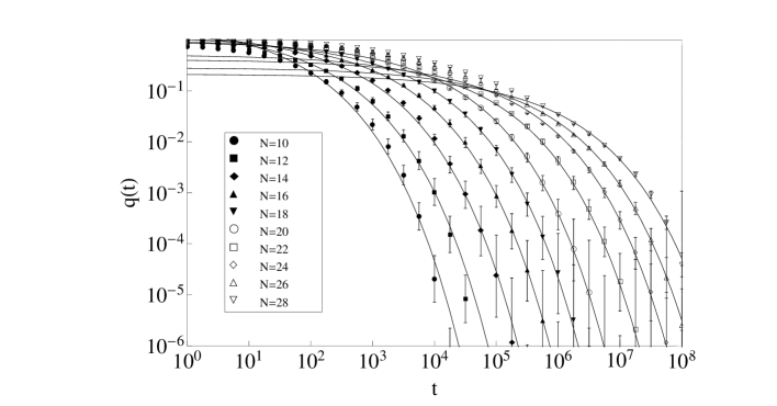
Figure 2: The relaxation of the autocorrelation function $\log q(N,t)$. Eqn.(16), against $\log(t)$ for $N$ from $10$ to $28$. .

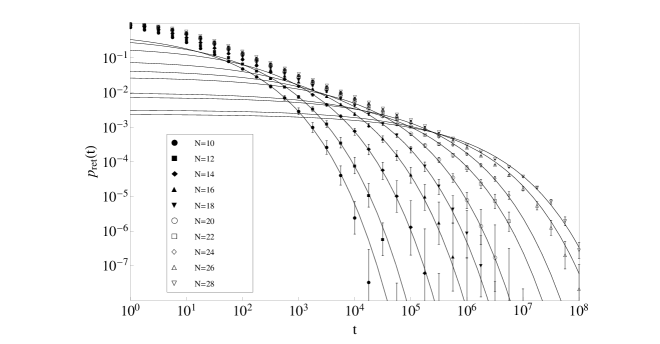
Figure 3: The decay of the return probability $\log p_{ret}(N,t)$, Eqn.(18), against $\log t$ for $N$ from $10$ to $28$.

In Figures 4 and 5 we present the same results in a different manner so as to demonstrate the stretched exponential long time behavior. On the $x$ axis the time scale is normalized with $x(t)=(t/\tau(N))^{1/3}$ and on the $y$ axis the measured $q(N,t)$ or $p_{ret}(N,t)$ are normalized so $y(N,t)=\ln(q(N,t)/A_{q}(N))$ and $y(N,t)=\ln(p_{ret}(N,t)/A_{ret}(N))$ respectively. In these plots a stretched exponential with exponent $1/3$ is a straight line as observed; we have chosen the normalization factors $\tau(N)$ and $A_{q}(N),A_{ret}(N)$ so that data for different hypercube dimensions $N$ collapse. This form of plot allows one to distinguish clearly between the short time regime and the stretched exponential regime; the latter can be seen to extend over a wide time range until measurements are limited by the statistical noise. The effective exponent $\beta=1/3$ is independent of $N$ to within the statistics.

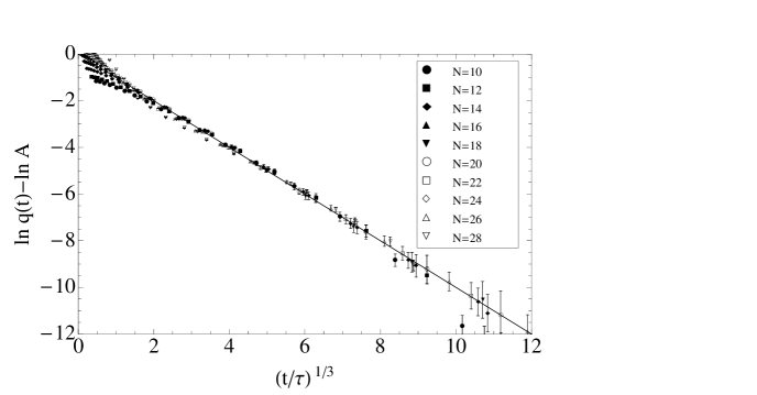
Figure 4: The decay of the normalized autocorrelation function $\ln(q(N,t)/A_{q}(N))$ against $(t/\tau)^{1/3}$. For stretched exponentials with exponent $\beta=1/3$ in the long time regime the data should lie on a straight line in this form of plot, as observed.

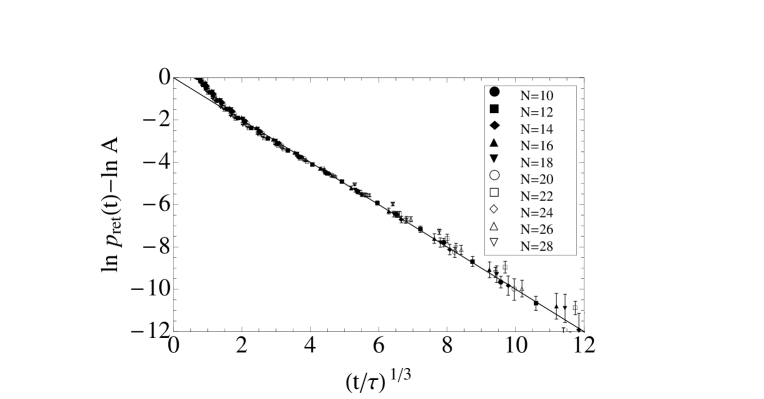
Figure 5: The decay of the normalized return probability $\log(p_{ret}(N,t)/A_{ret}(N))$ against $(t/\tau(N))^{1/3}$. For stretched exponentials with exponent $\beta=1/3$ in the long time regime the data should lie on a straight line on this form of plot, as observed.

On Figure 6 we show the size dependence on the $\tau(N)$ time scale parameter from the fits of the autocorrelation $q(t,N)$ and the return probability $p_{ret}(t,N)$ data. The data can be fitted by fitted by

$$\tau(N)=B10^{\gamma N}$$ (24)

with the fit parameters $\gamma=0.24\pm 0.1$ and $B=1.5\pm 0.1$ for autocorrelation function, $\gamma=0.24\pm 0.05$ and $B=1.7\pm 0.2$ for the return probability. The values of the time scaling parameters $\tau(N)$ for the two different observables are identical within the precision of the measurements.

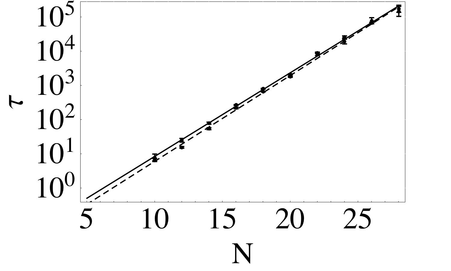
Figure 6: The dependence of the time scale $\tau(N)$ with dimension for the return probability $p_{ret}(N,t)$ (in red) and autocorrelation $q(N,t)$ (in blue).

The most fundamental way to understand the system dynamics is through investigating the eigenvalue spectra; the stretched exponential long time behavior depends exclusively on the density of the eigenvalues above the smallest eigenvalue, in the region where the distribution for a finite size sample can still be considered to be continuous. A given spectrum leads unambiguously to a unique relaxation function, while it is much more difficult to determine the precise form of a mode spectrum from a relaxation function.

On Figure 7 we compare the mode density $\rho(s)$ obtained through the present simulations with the theoretical expressions. All the numerical results were obtained using $1000$ different realizations of the diluted hypercube at each dimension $N$. Unfortunately in practice the calculations of $\rho(s)$ are numerically demanding because of strong sample to sample fluctuations. The spectra were first binned in the form of histograms. We defined a cut-off $\lambda_{min}(N)$ or equivalently $s_{max}(N)=-\ln\lambda_{min}(N)$ to eliminate the short time effects and selected the eigenvalues on the interval $s\in(0,s_{max}(N))$. We choose $s_{max}=2/\tau(N)$ for all dimensions. We divided this interval in bins equally spaced on a logarithmic scale and then calculated the densities for each interval, normalizing the frequencies by the length of the intervals.

The continuous curves were calculated from the expression (4) for $\rho_{K,1/3}(\lambda)$ and from the approximate analytic expression (6) for $\rho_{S}(\lambda)$ using $\tau(N)$ estimated from equation (24). To compare with simulation results we normalized $\rho(\lambda)$ functions using:

$$C^{-1}=\int_{0}^{s_{max}}\rho(s)ds$$ (25)

and

$$\rho^{\prime}(s)=C\rho(s)$$ (26)

Over the ranges for which reliable data points have been obtained the measured mode spectrum densities $\rho(N,s)$ closely resemble the corresponding parts of the calculated spectra from the Laplace transform $\rho_{K,1/3}(s)$, (4) or the analytic $\rho_{S}(s)$ spectrum (6) samukhin2008 (which are in fact very similar to each other). The numerical spectra for the hypercube model are indeed consistent with the mode density spectral form derived analytically for the more general random network model samukhin2008 .

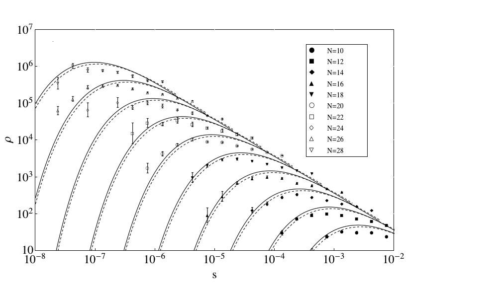
Figure 7: Spectral density data $\rho(N,s)$ from the hypercube evaluations together with the exact Laplace transforms $\rho_{1/3}(s)$ (4) for stretched exponentials with $\beta=1/3$ and $\tau(N)$ values equal to the numerical estimates 24 (dashed lines), and the analytic sparse network expression (6),samukhin2008 (full lines). The values are normalized (see text).

Discussion and conclusions

We have studied numerically relaxation through random walks along near neighbor edges on the giant cluster of vertices in randomly diluted hypercubes of dimensions up to $N=28$ near the percolation threshold for the cluster. The data show clearly that at the percolation threshold concentration $p_{c}(N)$, the relaxation mode spectrum, the time dependence of the autocorrelation $q(N,t)$, and the return probability $p_{ret}(N,t)$, are all consistent with asymptotic stretched exponential relaxation $\exp[-(t/\tau(N))^{\beta}]$ having exponent $\beta=1/3$. The time scale $\tau(N)$ increases exponentially with dimension $N$, Eqn. (24). The observed eigenvalue spectra demonstrate that the dynamical $q(N,t)$ behavior previously obtained from Monte Carlo simulations and from numerical solutions of the master equation lemke1996 ; lemke2000 ; almeida2000 does not represent a crossover between different exponential regimes, but that it is the consequence of a specific wide eigenvalue spectrum.

A final long time crossover to a pure exponential (which would correspond to a regime where the effective relaxation mode spectrum is reduced to a gap between the ground state and the lowest mode) is not visible in the data.

This diluted hypercube model at threshold can be considered as the limiting high dimensional case of percolation on sphere-like spaces. Alternatively it can be considered as a specific explicit example of a generic sparse random network. The observed stretched exponential behavior with exponent $\beta=1/3$ on the dilute hypercube at the percolation threshold is consistent with the predictions of the sphere-like percolation approach ian1 and with studies of random walks on sparse random networks bray1988 ; samukhin2008 , where the same stretched exponential relaxation with the same exponent $\beta=1/3$ has been derived analytically.

For a physical system, configuration space can be imagined as a very high dimensional graph. The system’s dynamics is equivalent to a random walk of the point representing the instantaneous state of the system among those vertices of the graph which are thermodynamically accessible. We suggest that when the stretched exponential $\exp[-(t/\tau)^{1/3}]$ form of limiting relaxation with diverging $\tau$ is observed numerically or experimentally for the autocorrelation function relaxation $q(t)$ in complex physical systems (which is often the case, see for instance ogi1985 ; angelani ; billoire )it is the signature of a configuration space tending to a percolation threshold and having a sparse random network topology.

References

- (1) R. Kohlrausch, Pogg. Ann. Phys. Chem. 91, 179 (1854).
- (2) F. Kohlrausch, Pogg. Ann. Phys. Chem. 119, 337 (1863).
- (3) W. Weibull, J. Appl. Mech. 18, 293 (1951).
- (4) Eliazar and Klafter Phys.Rev.E 77, 061125 (2008).
- (5) G. Williams and D.C. Watts, Trans. Faraday Soc. 66, 80 (1970).
- (6) R.V. Chamberlin, G. Mozurkewich, and R. Orbach, Phys. Rev. Lett. 52, 867 (1984).
- (7) A.T. Ogielski, Phys. Rev. B 32, 7384 (1985).
- (8) J.C. Phillips, Rep. Prog. Phys. 59, 1133 (1996).
- (9) A. Bunde, S. Havlin, J. Klafter, G. Gräff, and A. Shehter, Phys. Rev. Lett. 78, 3338 (1998).
- (10) J.C. Rasaiah, J. Zhu, J.B. Hubbard, and R.J. Rubin, J. Chem. Phys. 93, 5768 (1990).
- (11) M.D. Donsker and S.R.S. Varadhan, Commun. Pure Appl. Math. 28, 525 (1975).
- (12) M.D. Donsker and S.R.S. Varadhan, Commun. Pure Appl. Math. 32, 721 (1979).
- (13) P. Grassberger and I. Procaccia, J. Chem. Phys. 77, 6281 (1982).
- (14) W. Götze and L. Sjögren, Rep. Prog. Phys. 55, 241 (1992).
- (15) I. A. Campbell, J.M. Flesselles, R. Jullien, and R. Botet, J. Phys. C: Solid State Phys. 20, L47 (1987).
- (16) I.A. Campbell, Europhys. Lett. 21, 959 (1993).
- (17) I.A. Campbell and L. Bernardi, Phys. Rev. B 50, 12643 (1994).
- (18) P. Erdös and A. Rényi, Magyar Tud. Akad. Mat. Kutató Int. Közl. 5 17 (1960), P. Eördos and J. Spencer, Comput.Math. Appl. 5, 33 (1979).
- (19) S. Alexander and R. Orbach, J. Phys. Lett. 43, L625 (1982); Y. Gefen, A. Aharony and S. Alexander, Phys. Rev. Lett. 50, 77 (1983).
- (20) P. Debye, Polar molecules, Dover(London) (1929)
- (21) J.-M. Caillol, J.Phys.A:Math.Gen, 37, 3077 (2004).
- (22) P. Jund, R. Jullien and I.A. Campbell, Phys.Rev. E 63 036131 (2001).
- (23) A. N. Samukhin, S.N. Dorogovtsev and J.F.F. Mendes, Physical Review E 77, 036115 (2008).
- (24) A.J. Bray and G.J. Rodgers, Phys Rev B 38, 11461(1988).
- (25) H. Pollard, Bull. Am. Math. Soc. 52, 908 (1946).
- (26) M. N. Berberan-Santos, Chem. Phys. Lett. 460, 146-150 (2008).
- (27) N. Lemke and I. A. Campbell, Physica A 230, 554 (1996).
- (28) R. M. C. de Almeida and N. Lemke and I. A. Campbell, 30, 701, Brazilian Journal of Physics (2000).
- (29) R.M.C. de Almeida and N. Lemke and I. A. Campbell, Eur. J. Phys. B, 18, 513, 2000.
- (30) B. Bollobás, Trans. Amer. Math. Soc. 286, 257 (1984).
- (31) C. Borgs, J. T. Chayes, R. van der Hofstad, G. Slade and J. Spencer, Combinatorica 26, 395 (2006).
- (32) D. Gaunt and R. Brak, J. Phys. A-Math. Gen. 17, 1761 (1984).
- (33) D. S. Gaunt, M. F. Skiis, and H. Ruskin, J. Phys A 9, 1899 (1976).
- (34) P. Grassberger, Physical Review E 67, 036101 (2003).
- (35) L. Angelani, G.Parisi, G. Ruocco and G. Viliani, Phys. Rev. Lett. 81, 4648 (1998).
- (36) Alain Billoire and I.A. Campbell, arXiv:1105.1902.