Scalar Wave Propagation in Random, Amplifying Media: Influence of Localization Effects on Length and Time Scales and Threshold Behavior

Abstract

We present a detailed discussion of scalar wave propagation and light intensity transport in three dimensional random dielectric media with optical gain. The intrinsic length and time scales of such amplifying systems are studied and comprehensively discussed as well as the threshold characteristics of single- and two-particle propagators. Our semi-analytical theory is based on a self-consistent Cooperon resummation, representing the repeated self-interference, and incorporates as well optical gain and absorption, modeled in a semi-analytical way by a finite imaginary part of the dielectric function. Energy conservation in terms of a generalized Ward identity is taken into account.

I Introduction

Built on a wide story of success and plenty of achievements in science, light propagation and intensity transport in multiple-light-scattering random media further provides a lot of remarkable and fascinating features in theory Tiggelen0602 ; Tiggelen0603 ; sergei ; Frank06 and experiment maret0601 ; maret0602 . Special ongoing interest is focused on optical gain material regarding disordered as well as periodic structures Cao03b ; Lagendijk_mie ; cao06 ; cao05 ; cao04 .

In theoretical physics a profound understanding of this subject requires the discussion of strong or Anderson localization And58 of light, a microscopic transport theory in the diffusive limit usually based on conservation laws, incorporation of gain or absorption into generalized conservation laws, as well as observing the occurrence of a threshold behavior of the light intensity.

Anderson localization has been shown gangof4 ; Vol80 to originate from repeated self-interference of diffusive modes. In experimentsWie97 ; Sch99 ; Wie99 the authors have tested this. Since intensity diffusion is solely based on energy conservation, a rigorous and consistent framework is needed to describe the interplay between coherent amplification and localization. Especially since coherent amplification is expected to enhance transmission whereas localization tends to stop light transport altogether. This interesting subjectBeenakker96 is also discussed in the context of random lasing Cao03b ; Cao00 , where it has been shown by measuring the photon statistics Cao01STAT , that the laser emission is due to coherent feedback and occurs from spatially confined spots in the sample. A theoretical attemptApalkov02 to independently explain such phenomena has been proposed based on scatterers statistically forming ring resonators within the sample, which is able to provide a feedback mechanism.

Despite the issue of transport and localization, also the onset of lasing behavior, the crossing of the so-called laser threshold, has triggered still ongoing publications Nussenzveig ; Lai ; Vahala ; Lagendijk_mie for the last decades. On the theoretical side, the difficulty lies in the use of static gain below threshold, which is perfectly valid unless the threshold is reached. Beyond the laser threshold, the laser dynamics have to be explicitely taken into account. Such a threshold behavior has to be carefully respected and incorporated in a consistent way into any theory of transport and localization.

In the present paper we clarify this subject by presenting a semi-analytical general theory of light propagation, localization effects in the presence of optical gain, and consistently discuss the occurrence and influence of a growth threshold on the single particle propagator as well as on the energy density correlation function, related to the intensity in the sample. In this way we set the last stage within the range of linear response theory, which then will serve as a basis to involve the actual lasing dynamics. This dynamical behavior is, however, not subject of this article and will be presented in forthcoming publication.

II Model and Theory

II.1 Basic Setup

Systems of significant experimental relevance maret0601 ; maret0602 ; Cao03b ; Lagendijk_mie ; cao06 ; cao05 ; cao04 consist of (almost) spherical scatterers embedded into a background medium forming some emulsion. For a theoretical description we therefore consider identical spherical scatterers located at random positions. The scatterers as well as the background medium are respectively assumed to be homogeneous and hence will be described by dielectric constants $\epsilon_{s}$ and $\epsilon_{b}$, respectively. Within a semiclassical context linear absorption and optical gain will be represented by a finite positive or negative part of the dielectric function, so in general ${\rm Im}\epsilon_{s}\neq 0\neq{\rm Im}\epsilon_{b}$ is assumed. Throughout the paper we neglect polarization effects and therefore consider the scalar wave equation which has been Fourier transformed from time $t$ to frequency $\omega$ and reads

$$\frac{\omega^{2}}{c^{2}}\,\epsilon(\vec{r}\,)\Psi_{\omega}(\vec{r}\,)+\nabla^{2}\Psi_{\omega}(\vec{r}\,)=-i\omega\frac{4\pi}{c^{2}}j_{\omega}(\vec{r}\,)\ ,$$ (1)

where $c$ denotes the vacuum speed of light and $j_{\omega}(\vec{r}\,)$ the current. The dielectric constant $\epsilon(\vec{r}\,)=\epsilon_{b}+\Delta\epsilon\,V(\vec{r}\,)$, where the dielectric contrast has been defined as $\Delta\epsilon=\epsilon_{s}-\epsilon_{b}$, describes the arrangement of scatterers through the function $V(\vec{r}\,)=\sum_{\vec{R}}S_{\vec{R}}\,(\vec{r}-\vec{R}\,)$, with $S_{\vec{R}}\,(\vec{r}\,)$ a localized shape function at random locations $\vec{R}$. The intensity is then related to the field-field-correlation function $\langle\Psi(\vec{r},\,t\,)\Psi^{*}(\vec{r}\,^{\prime},t\,^{\prime}\,)\rangle$ here angular brackets $\langle\ldots\rangle$ denote ensemble or disorder average. To calculate the field-field-correlation the Green’s function formalism is best suited, the (single-particle) Green’s function is related to the (scalar) electrical field by

$$\Psi(\vec{r},\,t\,)=\left\lmoustache\!{\rm d}^{3}r\,^{\prime}\right.\!\!\left\lmoustache\!{\rm d}t\,^{\prime}\right.G(\vec{r}\,,\vec{r}\,^{\prime}\,;\,t\,,t^{\prime}\,)j(\vec{r}\,^{\prime}\,,t^{\prime}\,)\,.$$ (2)

The Fourier transform of the retarded, disorder averaged single-particle Green’s function of Eq. (1) reads,

$$G_{\vec{q}}^{\omega}=\frac{1}{\epsilon_{b}(\omega/c)^{2}-|\vec{q}|^{2}-\Sigma^{\omega}_{\vec{q}}}\ ,$$ (3)

where the retarded self-energy $\Sigma_{\vec{q}}^{\omega}$ arises from scattering off the random “potential” $-(\omega/c)^{2}(\epsilon_{s}-\epsilon_{b})V(\vec{r}\,)$. Using the Green’s function the mode density $N(\omega)$ may be expressed as $N(\omega)=-(\omega/\pi){\rm Im}G_{0}^{\omega}$, with the abbreviation used throughout this publication $G_{0}^{\omega}\equiv\int d^{3}q/(2\pi)^{3}\,G_{\vec{q}}^{\omega}$.

In order to study the transport of the above introduced field-field-correlation we consider the so-called 4-point correlation function, defined in terms of the non-averaged Green’s functions $\hat{G}$, $\hat{G}^{*}$ in momentum and frequency space as $\Phi^{\omega}_{\vec{q}\vec{q}^{\prime}\,\,}(\vec{Q},\Omega)=\langle\hat{G}^{\omega_{+}}_{{\vec{q}}_{+}{\vec{q}}_{+}^{\,\prime}}\hat{G}^{\omega_{-}\,*}_{{\vec{q}}_{-}^{\,\prime}{\vec{q}}_{-}}\rangle$. Here we have introduced the usual Lubatsch05 center-of-mass ($\vec{q}$, $\omega$) and relative ($\vec{Q}$, $\Omega$) frequencies and momenta: The variables $\Omega$, $\vec{Q}$ are associated with the time and position dependence of the averaged energy density, with $\hat{Q}=\vec{Q}/|\vec{Q}|$, while $\omega_{\pm}=\omega\pm\Omega/2$ and $\vec{q}_{\pm}=\vec{q}\pm\vec{Q}/2$ etc. are the frequencies and momenta of in- and out-going waves, respectively.

The intensity correlation, or disorder averaged particle-hole Green’s function, $\Phi^{\omega}_{\vec{q}\vec{q}^{\prime}}(\vec{Q},\Omega)$ obeys the so-called Bethe-Salpeter equation

$$\!\!\!\!\!\!\!\!\!\!\!\!\!\!\!\!\!\!\!\!\!\!\!\!\!\!\!\!\!\!\!\!\!\!\!\!\Phi_{\vec{q}\vec{q}^{\prime}}\,=\,G^{R}_{q_{+}}(\omega_{+})G^{A}_{q_{-}}(\omega_{-}){\color[rgb]{1,1,1}0000000000000000}$$

$$\!\qquad{\color[rgb]{1,1,1}00000000}\left[\delta(\vec{q}-\vec{q}\prime)+\left\lmoustache\frac{{\rm d}^{3}q\,^{\prime\prime}\,}{(2\pi)^{3}}\right.\gamma_{q\,q\,^{\prime\prime}\,}\Phi_{\vec{q}\,^{\prime\prime}\,\vec{q}\,^{\prime}\,}\right]\,.$$ (4)

By utilizing the known averaged single particle Green’s function, c.f. Eq. (3), on the left-hand side of Eq. (II.1) the Bethe-Salpeter equation may be rewritten as kinetic equation, see, e.g., Ref. Lubatsch05 ,

$$\left[\omega\Omega\frac{{\rm Re}{\epsilon_{b}}}{c^{2}}-Q\,(\vec{q}\cdot\hat{Q})+\frac{i}{c^{2}\tau^{2}}\right]\Phi^{\omega}_{\vec{q}\vec{q}^{\prime}} =$$ (5)

$$-i{\rm Im}G^{\omega}_{\vec{q}}\left[\delta(\vec{q}-\vec{q}\prime)+\left\lmoustache\frac{{\rm d}^{3}q^{\prime\prime}}{(2\pi)^{3}}\right.\gamma^{\omega}_{\vec{q}{\vec{q}^{\prime\prime}}}\Phi^{\omega}_{\vec{q}^{\prime\prime}\vec{q}^{\prime}}\right].$$

In order to analyze the correlation function’s long-time ($\Omega\to 0$) and long-distance ($|\vec{Q}|\to 0$) behavior, terms of $O(\Omega^{2},Q^{3},\Omega Q)$ have been neglected here and throughout this paper. Eq. (5) contains both, the total quadratic momentum relaxation rate $1/\tau^{2}=c^{2}\,{\rm Im}(\epsilon_{b}\omega^{2}/c^{2}-\Sigma^{\omega})$ (due to absorption/gain in the background medium as well as impurity scattering) and the irreducible two-particle vertex function $\gamma^{\omega}_{\vec{q}\vec{q}^{\,\prime}}(\vec{Q},\Omega)$.

To solve this equation, the technique of expansion into moments is used. The technical details of this expansion are discussed in the following subsection B. The Reader not interested in such details may skip this and readily proceed to subsection C.

Furthermore it is to be noted that the energy conservation is implemented into the solution of the Bethe-Salpeter equation in a field theoretical sense by a Ward identity (WI) which has been derived for the photonic case in Ref. Lubatsch05, , and which for scalar waves takes the exact form

$$\Sigma^{\omega_{+}}_{\vec{q}_{+}}-\Sigma^{\omega_{-}\,*}_{\vec{q}_{-}}\!\! - \!\!\left\lmoustache\!\!\frac{{\rm d}^{3}q^{\prime}}{(2\pi)^{3}}\right.\left[G^{\omega_{+}}_{{\vec{q}}_{+}^{\,\prime}}-G^{\omega_{-}\,*}_{{\vec{q}}_{-}^{\,\prime}}\right]\,{\gamma}^{\omega}_{{\vec{q}}^{\,\prime}{{\vec{q}}}}({\vec{Q}},\Omega)$$

$$= \!\!\!f_{\omega}(\Omega)\!\left[\!{\rm Re}{\Sigma}^{\omega}_{{\vec{q}}}\!+\!\!\left\lmoustache\!\!\frac{\rm d^{3}q^{\prime}}{(2\pi)^{3}}\right.{\rm Re}{G}^{\omega}_{{\vec{q}}^{\,\prime}}\,{\gamma}^{\omega}_{{\vec{q}}^{\,\prime}{{\vec{q}}}}({\vec{Q}},\Omega)\right]\!.$$

The right-hand side of Eq. (II.1) represents reactive effects (real parts), originating from the explicit $\omega^{2}$-dependence of the photonic random “potential”. In conserving media (${\rm Im}\epsilon_{b}={\rm Im}\epsilon_{s}=0$) these terms renormalize the energy transport velocity $v_{\mbox{\tiny E}}$ relative to the average phase velocity $c_{p}$ without destroying the diffusive long-time behavior.Kro93 ; Lubatsch05 In presence of loss or gain, however, these effects are enhanced via the prefactor $f_{\omega}(\Omega)=(\omega\Omega{\rm Re}\Delta\epsilon+i\omega^{2}{\rm Im}\Delta\epsilon)/(\omega^{2}{\rm Re}\Delta\epsilon+i\omega\Omega{\rm Im}\Delta\epsilon)$, which now does not vanish in the limit $\Omega\to 0$.

Figure 1: Ladder approximation of the total particle-hole vertex. The diagrams on the left-hand side form a geometrical series and may therefore easily be summed up analytically.

II.2 Expansion of Two-particle Green’s Function into Moments

In order to extract a diffusion pole structure out of the Bethe-Salpeter equation Eq. (II.1), the correlator or equivalently the $\vec{q}\,^{\prime}\,$ integrated correlator

$$\Phi_{\vec{q}}=\left\lmoustache\!\!\frac{{\rm d}^{3}q\,^{\prime}\,}{(2\pi)^{3}}\right.\!\!\Phi_{\vec{q\,}\vec{q}\,^{\prime}\,}$$ (7)

has to be decoupled from the momentum dependent prefactors with the help of some approximation scheme. In this subsection we discuss this procedure in analogy to the argumentation for electronic correlations presented in reference Kopp . Such an approximation must obey the results of the so-called ladder approximation as well as it must incorporate the set of physical relevant variables involved in observed phenomena. In a first step we use the bare first two moments of the correlation function $\Phi_{\vec{q}}$ defined according to

$$\Phi_{\rho\rho}(\vec{Q},\Omega) = \left\lmoustache\!\frac{{\rm d}^{3}q}{(2\pi)^{3}}\right.\!\!\left\lmoustache\!\frac{{\rm d}^{3}q\,^{\prime}}{(2\pi)^{3}}\right.\Phi_{\vec{q}\,\vec{q}\,^{\prime}\,}$$ (8)

$$\Phi_{j\rho}(\vec{Q},\Omega) = \left\lmoustache\!\frac{{\rm d}^{3}q}{(2\pi)^{3}}\right.\!\!\left\lmoustache\!\frac{{\rm d}^{3}q\,^{\prime}}{(2\pi)^{3}}\right.(\vec{q}\cdot\hat{Q})\Phi_{\vec{q}\,\vec{q}\,^{\prime}\,},$$ (9)

respectively. The second step is to recognize that these bare moments are related to physical quantities, the energy density correlation $P^{\omega}_{\mbox{\tiny E}}(\vec{Q},\Omega)$ and the current-density-correlation $J^{\omega}_{\mbox{\tiny E}}(\vec{Q},\Omega)$, by dimensional prefactors:

$$P^{\omega}_{\mbox{\tiny E}}(\!\vec{Q},\Omega)\!\! = \!\!\left[\!\frac{\omega}{c_{\mbox{\tiny p}}}\!\right]^{2}\!\!\!\Phi_{\rho\rho}\,\,\,\,\Leftrightarrow\Phi_{\rho\rho}\!=\!\left[\!\frac{c_{\mbox{\tiny p}}}{\omega}\!\right]^{2}\!\!P^{\omega}_{\mbox{\tiny E}}(\!\vec{Q},\Omega)$$ (10)

$$J^{\omega}_{\mbox{\tiny E}}(\!\vec{Q},\Omega)\!\! = \!\!\left[\!\frac{\omega v_{\mbox{\tiny E}}}{c_{\mbox{\tiny p}}}\!\right]\!\Phi_{j\rho}\Leftrightarrow\Phi_{j\rho}\!=\!\left[\!\frac{c_{\mbox{\tiny p}}}{\omega v_{\mbox{\tiny E}}}\!\right]\!J^{\omega}_{\mbox{\tiny E}}(\!\vec{Q},\Omega)\,.$$ (11)

The projection of the correlator $\Phi_{\vec{q}}$, Eq. (7), onto the bare moments $\Phi_{\rho\rho}(\vec{q},\Omega)$ as defined in Eq. (8), and $\Phi_{j\rho}(\vec{q},\Omega)$, shown in Eq. (9), is therefore given by

$$\left\lmoustache\!\frac{{\rm d}^{3}q\,^{\prime}}{(2\pi)^{3}}\Phi_{\vec{q}\vec{q}\,^{\prime}}\right. \!\!=\!\! \frac{A(\vec{q}\,)}{\!\left\lmoustache\!\!\frac{{\rm d}^{3}q^{\prime}}{(2\pi)^{3}}\right.\!\!A(\vec{q}\,^{\prime})}\Phi_{\rho\rho}(\vec{Q},\Omega)$$

$$\!\!+\!\! \frac{B(\vec{q}\,)(\vec{q}\cdot\hat{Q})}{\!\left\lmoustache\!\!\frac{{\rm d}^{3}q^{\prime}}{(2\pi)^{3}}\right.\!\!B(\vec{q}\,^{\prime})(\vec{q}\,^{\prime}\cdot\hat{Q})^{2}}\Phi_{j\rho}(\vec{Q},\Omega),$$

where the projection coefficients $A(\vec{q}\,)$ and $B(\vec{q}\,)$ are to be determined in the following. For obvious reasons in this expansion the bare moments may be substituted by their physical counterparts energy density $P^{\omega}_{\mbox{\tiny E}}$ in Eq. (10) and current density $J^{\omega}_{\mbox{\tiny E}}(\vec{Q},\Omega)$ from Eq. (11). The expansion coefficients $A(\vec{q}\,)$ and $B(\vec{q}\,)$ in Eq. (II.2) behave uncritically under localization, so they can be determined using the simple ladder approximation, where all expressions are known exactly. The ladder approximation of the two-particle vertex function is explicitely illustrated in Fig. 1. In the following we use this approximation and demonstrate how to obtain the expansion coefficients from it. In ladder approximation the zeroth bare moment is given by:

$$\Phi_{\rho\rho}^{L}(\vec{Q},\Omega) = \left\lmoustache\!\frac{{\rm d}^{3}q}{(2\pi)^{3}}\right.\!\!\left[G_{\vec{q}_{+}}(\vec{Q},\Omega)G^{*}_{\vec{q}_{-}}(\vec{Q},\Omega)\right]^{2}\Gamma_{L}$$ (13)

$$= \frac{1}{\tilde{\gamma}_{0}^{2}}\Gamma_{L},$$

the superscript $L$ refers to the ladder approximation and in the last step the product $\left\lmoustache\!\frac{{\rm d}^{3}q}{(2\pi)^{3}}\right.\!\!\left[G_{\vec{q}_{+}}(\vec{Q},\Omega)G^{*}_{\vec{q}_{-}}(\vec{Q},\Omega)\right]^{2}$ has been expanded up to linear order in $\vec{q}$ furthermore the renormalized vertex $\tilde{\gamma}_{0}$ is given by

$$\tilde{\gamma}_{0} \!\!=\!\! \gamma_{0}\!+\!f_{\omega}(\Omega)\frac{\left(\!{\rm Re\,}\gamma_{0}G_{0}\!+\!{\rm Re\,}\Sigma\!\right)}{{\rm Im\,}G_{0}}\!-\!\frac{\omega^{2}{\rm Im\,}\epsilon_{b}}{{\rm Im\,}G_{0}}$$ (14)

where $\gamma_{0}$ is the bare vertex and $f_{\omega}(\Omega)$ arising from the Ward identity has been defined in Eq. (II.1). Within the simple ladder approximation the bare moment $\Phi^{L}_{j\rho}(\vec{Q},\Omega)$ defined in Eq. (9) is thus given by

$$\Phi^{L}_{j\rho}(\!\vec{Q},\Omega)\!\!=\!\!\!\left\lmoustache\!\frac{{\rm d}^{3}q}{(2\pi)^{3}}\right.\!\!(\vec{q}\cdot\hat{Q})G_{\vec{q}_{+}}\!G^{*}_{\vec{q}_{-}}\!\!\left\lmoustache\!\frac{{\rm d}^{3}q\,^{\prime}\,}{(2\pi)^{3}}\right.\!\!G_{\vec{q}\,^{\prime}_{+}}\!G^{*}_{\vec{q}\,^{\prime}_{-}}\!\!\Gamma_{L}\,.$$ (15)

Following the above strategy and expanding the product $G_{\vec{q}\,^{\prime}_{+}}G^{*}_{\vec{q}\,^{\prime}_{-}}$ under the second integral up to first order in $\vec{q\,}^{\prime}$ one obtains the expression

$$\Phi^{L}_{j\rho}(\vec{Q},\Omega)=\frac{1}{\tilde{\gamma}_{0}}\Gamma_{L}\!\left\lmoustache\!\frac{{\rm d}^{3}q}{(2\pi)^{3}}\right.\!\!(\vec{q}\cdot\hat{Q})G_{\vec{q}_{+}}G^{*}_{\vec{q}_{-}}$$ (16)

By now employing the same expansion to the remaining product of the Green’s function one eventually finds

$$\Phi^{L}_{j\rho}(\vec{Q},\Omega)=\frac{\Gamma_{L}}{\tilde{\gamma}_{0}}\!\left\lmoustache\!\frac{{\rm d}^{3}q}{(2\pi)^{3}}\right.\!\!(\vec{q}\cdot\hat{Q})\frac{1}{2}\frac{\Delta G_{\vec{q}}^{2}(\vec{q}\cdot\hat{Q})Q}{\tilde{\gamma}_{0}\Delta G_{0}},$$ (17)

where the abbreviation $\Delta G\equiv G-G^{*}$ has been introduced and will be used throughout this paper.

In the next step of determining the expansion coefficients $A(\vec{q}\,)$ and $B(\vec{q}\,)$ defined in Eq. (II.2) we go back to the field-field correlation function $\Phi_{\vec{q}\vec{q}\,^{\prime}\,}$. Within the uncritical ladder approximation the two particle Green’s function is given by

$$\!\left\lmoustache\!\frac{{\rm d}^{3}q\,^{\prime}}{(2\pi)^{3}}\right.\!\!\Phi_{\vec{q}\vec{q}\,^{\prime}}=\left[G_{\vec{q}_{+}}G^{*}_{\vec{q}_{-}}\right]\Gamma_{L}\!\left\lmoustache\!\frac{{\rm d}^{3}q\,^{\prime}}{(2\pi)^{3}}\right.\!\!G_{\vec{q}\,^{\prime}_{+}}G^{*}_{\vec{q}\,^{\prime}_{-}}.$$ (18)

Employing again the momentum expansion of the single-particle Green’s function the above equation, Eq. (18) can be simplified to yield

$$\Phi_{\vec{q}}=\frac{\Delta G_{\vec{q}}}{\tilde{\gamma}_{0}^{2}\Delta G_{0}}\Gamma_{L}+\frac{1}{2}\frac{\Delta G_{\vec{q}}^{2}(\vec{q}\cdot\hat{Q})Q}{\tilde{\gamma}_{0}^{2}\Delta G_{0}}\Gamma_{L}.$$ (19)

Finally we are in the position to start putting things together. By using the above given momentum expansion, Eq. (19), together with the expressions given in Eq. (17) and in Eq. (13) in conjunction with the proposed projection, or expansion into moments, Eq. (II.2), the following relation is eventually obtained

$$\frac{\Delta G_{\vec{q}}}{\tilde{\gamma}_{0}^{2}\Delta G_{0}}\Gamma_{L}+\frac{1}{2}\frac{\Delta G_{\vec{q}}^{2}(\vec{q}\cdot\hat{Q})Q}{\tilde{\gamma}_{0}^{2}\Delta G_{0}}\Gamma_{L}$$ (20)

$$=\!\frac{A(\vec{q}\,)}{\!\left\lmoustache\!\!\frac{{\rm d}^{3}q^{\prime}}{(2\pi)^{3}}\right.\!\!A(\vec{q}\,^{\prime})}\frac{1}{\tilde{\gamma}_{0}^{2}}\Gamma_{L}$$

$$+\frac{B(\vec{q}\,)(\vec{q}\cdot\hat{Q})}{\!\left\lmoustache\!\!\frac{{\rm d}^{3}q^{\prime}}{(2\pi)^{3}}\right.\!\!B(\vec{q}\,^{\prime})(\vec{q}\,^{\prime}\cdot\hat{Q})^{2}}\frac{\Gamma_{L}}{\tilde{\gamma}_{0}}\!\left\lmoustache\!\frac{{\rm d}^{3}q}{(2\pi)^{3}}\right.\!\!(\vec{q}\cdot\hat{Q})\frac{1}{2}\frac{\Delta G_{\vec{q}}^{2}(\vec{q}\cdot\hat{Q})Q}{\tilde{\gamma}_{0}\Delta G_{0}}\,.$$

By comparison of coefficients in the above relation, Eq. (20), the demanded coefficients $A({\vec{q}}\,)$ and $B({\vec{q}}\,)$ of the expansion into moments, Eq. (II.2), can now be determined to be

$$A({\vec{q}}\,)=\Delta G_{\vec{q}}\qquad B({\vec{q}}\,)=\Delta G_{\vec{q}}^{2}.$$ (21)

Employing those expressions for the expansion coefficients, one may eventually express the two-particle correlator $\Phi_{\vec{q}\vec{q}\,^{\prime}}$ in the following way

$$\!\left\lmoustache\!\frac{{\rm d}^{3}q^{\prime}}{(2\pi)^{3}}\right.\!\!\Phi_{\vec{q}\vec{q}\,^{\prime}} = \frac{\Delta G_{\vec{q}}}{\left(\frac{\omega}{c_{\mbox{\tiny p}}}\right)^{2}\!\left\lmoustache\!\!\frac{{\rm d}^{3}q\,^{\prime}}{(2\pi)^{3}}\right.\!\!\Delta G_{\vec{q}\,^{\prime}}}P^{\omega}_{\mbox{\tiny E}}(\vec{Q},\Omega)$$

$$+\frac{\Delta G_{\vec{q}}^{2}(\vec{q}\cdot\hat{Q})}{\left(\frac{\omega v_{\mbox{\tiny E}}}{c_{\mbox{\tiny p}}}\right)\!\left\lmoustache\!\!\frac{{\rm d}^{3}q\,^{\prime}}{(2\pi)^{3}}\right.\!\!\Delta G_{\vec{q}\,^{\prime}}^{2}(\vec{q}\,^{\prime}\cdot\hat{Q})^{2}}J^{\omega}_{\mbox{\tiny E}}(\vec{Q},\Omega).$$

The above expression, Eq. (II.2), represents the complete expansion of the intensity correlator into its moments. This will be used in the next subsection to decouple and therefore solve the Bethe-Salpeter equation.

II.3 General Solution of the Bethe-Salpeter Equation

The disorder averaged intensity correlation, the two-particle Green’s function, obeys the Bethe-Salpeter equation, see Eq. (II.1)

$$\Phi_{\vec{q}\,\vec{q}\,^{\prime}\,}\!\! = \!\!G_{q_{+}}^{\omega_{+}}G^{*\,\omega_{-}}_{q_{-}}\!\left[1\!\!+\!\!\!\left\lmoustache\!\!\frac{{\rm d}^{3}q\,^{\prime\prime}\,}{(2\pi)^{3}}\right.\!\!\gamma_{q\,q\,^{\prime\prime}\,}\Phi_{\vec{q}\,^{\prime\prime}\,\vec{q}\,^{\prime}}\right]$$ (23)

as already discussed the Bethe-Salpeter equation may be rewritten into the kinetic equation given in Eq. (5)

$$\!\!\!\!\!\!\!\!\!\!\!\!\!\!\!\!\!\!\!\left[\omega\Omega 2{\rm Re\,}\epsilon-Q\left(\vec{q}\cdot\hat{Q}\right)+\Delta\Sigma-\omega^{2}\Delta\epsilon\right]\Phi_{\vec{q}}$$

$$\qquad=\Delta G_{\vec{q}}+\left\lmoustache\!\!\frac{{\rm d}^{3}q\,^{\prime}}{(2\pi)^{3}}\right.\!\!\Delta G_{\vec{q}}\gamma_{\vec{q}\vec{q}\,^{\prime}\,}\Phi_{\vec{q}\,^{\prime}\,}\,.$$ (24)

To find the solution of Eq. (II.3), in a first step one sums in Eq. (II.3) over momenta $\vec{q}$, incorporates the generalized Ward identity as given in Eq. (II.1) and subsequently expands the obtained result for small internal momenta $Q$ and internal frequencies $\Omega$. It is also essential to employ the decoupling shown in Eq. (II.2). Eventually after some algebraic manipulations the generalized continuity equation for the energy density is found to be

$$\Omega P^{\omega}_{\mbox{\tiny E}}+QJ^{\omega}_{\mbox{\tiny E}}=\frac{4\pi i\,\omega\,N(\omega)}{g^{(1)}_{\omega}\left[1+\Delta(\omega)\right]c_{p}^{2}}\!\! + \!\!\frac{i[g^{(0)}_{\omega}+\Lambda(\omega)]}{g^{(1)}_{\omega}\left[1+\Delta(\omega)\right]}P^{\omega}_{\mbox{\tiny E}}$$

which represents energy conservation in the presence of optical gain and/or absorption.

Within the standard solution procedure the next step is to obtain a linearly independent equation which also relates the energy density $P^{\omega}_{\mbox{\tiny E}}$ and the current density $J^{\omega}_{\mbox{\tiny E}}$. This is realized in a similar way to above, foregoing one first multiplies the kinetic equation, Eq.(II.3), by the projector $\left[\vec{q}\cdot\hat{Q}\right]$ and then follows the above outlined recipe to eventually obtain the wanted second relation, this is the so-called current relaxation equation

$$\left[\omega\Omega\frac{{\rm Re}{\epsilon_{b}}}{c^{2}}+\frac{i}{c^{2}\tau^{2}}+iM(\Omega)\right]J^{\omega}_{\mbox{\tiny E}}\!\! + \!\!\tilde{A}\,QP_{\mbox{\tiny E}}^{\omega}=0\ ,$$ (26)

relating as demanded energy density $P^{\omega}_{\mbox{\tiny E}}$ and energy density current $J^{\omega}_{\mbox{\tiny E}}$ and furthermore introduces the so-called memory function $M(\Omega)$ according to

$$M\!(\Omega)\!=\!\frac{i\!\!\left\lmoustache\!\!\frac{{\rm d}^{3}q}{(2\pi)^{3}}\right.\!\!\!\left\lmoustache\!\!\frac{{\rm d}^{3}q\,^{\prime}}{(2\pi)^{3}}\right.\!\![\vec{q}\!\cdot\!\hat{Q}]\Delta G_{\vec{q}}^{\omega}\gamma^{\omega}_{\vec{q}\vec{q}\,^{\prime}}(\Delta G_{\vec{q}\,^{\prime}}^{\omega})^{2}[\vec{q}\,^{\prime}\!\cdot\!\hat{Q}]}{\left\lmoustache\!\!\frac{{\rm d}^{3}q}{(2\pi)^{3}}\right.[\vec{q}\!\cdot\!\hat{Q}]^{2}(\Delta G_{\vec{q}}^{\omega})^{2}}.$$ (27)

where $\gamma^{\omega}_{\vec{p}\vec{p}^{\prime}}\equiv\gamma^{\omega}_{\vec{p}\vec{p}^{\prime}}(\vec{Q},\Omega)$ is the total irreducible two-particle vertex, which will be discussed in more detail in the following subsection.

So far, two independent equations, Eq. (LABEL:continuityL) and Eq. (26), have been obtained, both of them relating the current density $J^{\omega}_{\mbox{\tiny E}}$ and density $P^{\omega}_{\mbox{\tiny E}}$. Therefore one may now eliminate one of the two variables in this linear system of equations. One chooses to combine the two equation to find an expression for the energy density

$$P_{\mbox{\tiny E}}^{\omega}(Q,\Omega)=\frac{4\pi iN(\omega)/(g^{(1)}_{\omega}\left[1+\Delta(\omega)\right]c_{p}^{2})}{\Omega+iQ^{2}D+i\xi_{a}^{-2}D}\ ,$$ (28)

exhibiting the expected diffusion pole structure for non-conserving media, i.e. in the denominator of Eq. (28) there appears an additional term as compared to the case of conserving media. This is the term $\xi_{a}^{-2}D$, sometimes referred to as the mass term, accounting for loss (or gain) to the intensity not being due to diffusive relaxation. In Eq. (28) also the generalized, $\Omega$-dependent diffusion coefficient $D(\Omega)$ has been introduced via the relation

$$D(\Omega)\left[1-i\,\Omega\omega\tau^{2}{\rm Re}\epsilon_{b}\right]=D_{0}^{tot}-c^{2}\tau^{2}D(\Omega)M(\omega).$$ (29)

Furthermore, Eq. (28) also introduces the absorption or gain induced growth or absorption scale $\xi_{a}$ of the diffusive modes,

$$\xi_{a}^{-2} = \frac{r_{\epsilon}A_{\epsilon}-2\omega^{2}{\rm Im}\epsilon_{b}}{2{\rm Re}\epsilon_{b}-A_{\epsilon}B_{\epsilon}/\omega}\ \frac{1}{\omega D(\Omega)},$$ (30)

which is to be distinguished from the single-particle or amplitude absorption or amplification length. The diffusion constant without memory effects in Eq. (29), $D_{0}^{tot}=D_{0}+D_{b}+D_{s}$, consists of the bare diffusion constant Kro93 ,

$$D_{0}=\frac{2v_{\mbox{\tiny E}}c_{p}}{\pi N(\omega)}\left\lmoustache\!\!\frac{{\rm d}^{3}q}{(2\pi)^{3}}\right.[\vec{q}\cdot\hat{Q}]^{2}({\rm Im}G_{\vec{q}}^{\omega})^{2}$$ (31)

and renormalizations from absorption or gain in the background medium ($D_{b}$) and in the scatterers ($D_{s}$),

$$D_{b}=\left(\omega\tau\right)^{2}\,{\rm Im}\epsilon_{b}\,\tilde{D}_{0}/4\ ,\qquad D_{s}=r_{\epsilon}A_{\epsilon}\tau^{2}\tilde{D}_{0}/8\ ,$$ (32)

where $\tilde{D}_{0}$ is the same as in Eq. (31), with $({\rm Im}G_{\vec{q}}^{\omega})^{2}$ replaced by ${\rm Re}(G_{\vec{q}}^{\omega\,2})$. In the above Eqs. (30)-(32) the following short-hand notations have been introduced,

$$u_{\epsilon} = \frac{{\rm Im}(\Delta\epsilon\Sigma^{\omega})}{{\rm Im}(\Delta\epsilon G_{0}^{\omega})}\ ,\qquad\qquad r_{\epsilon}={{\rm Im}\Delta\epsilon}/{{\rm Re}\Delta\epsilon},$$

$$A_{\epsilon} = 2[u_{\epsilon}{\rm Re}G_{o}+{\rm Re}\Sigma_{o}]$$

$$B_{\epsilon} = \frac{({\rm Re}\Delta\epsilon)^{2}+({\rm Im}\Delta\epsilon)^{2}}{2\omega^{2}({\rm Re}\Delta\epsilon)^{2}}.$$

II.4 Vertex Function and Self-consistency

Figure 2: The upper panel shows a diagrammatic expansion of the irreducible two-particle vertex $\gamma$. The lower panel displays the disentangled Cooperon with changed momentum arguments as discussed in the text below.

From equations Eq. (27) and Eq. (29) it is clear that the energy density or two-particle function given in Eq. (28) still depends on the full two-particle vertex $\gamma^{\omega}_{{\vec{q}}^{\,\prime}{{\vec{q}}}}$. Before discussing the vertex function, we want to briefly recall some arguments concerning dissipation. As a simplified argument to better understand the physical content of the presented systems, one might consider a damped harmonic oscillator. The damping term clearly introduces dissipation as it breaks time reversal symmetry. However, the time reversed solution is still damped with the very same damping constant. This shows that the dissipation rate itself is invariant under time reversal, which at first sight might sound surprising.

Bearing this in mind one may carefully analyze the vertex $\gamma^{\omega}_{{\vec{q}}^{\,\prime}{{\vec{q}}}}$ for the self-consistent calculation of $M(\Omega)$ Vol80 ; Kro90 , exploiting time reversal symmetry of propagation in the active medium. In the long-time limit ($\Omega\to 0$) the dominant contributions to $\gamma^{\omega}_{{\vec{q}}^{\,\prime}{{\vec{q}}}}$ are the same maximally crossed diagrams (Cooperons) as for conserving media, which may also be disentangled. In Fig. (2) the disentangling of the Cooperon into the regular diffusion ladder is demonstrated. The internal momentum argument of the disentangled irreducible vertex function in the second line of Fig. (2) is replaced by the new momentum $\vec{Q}=\vec{k}+\vec{k}^{\prime}$ . By the described procedure $\gamma^{\omega}_{{\vec{q}}^{\,\prime}{{\vec{q}}}}$ now acquires the absorption (gain)-induced decay (growth) rate $\xi_{a}^{-2}D$. Finally the memory kernel $M(\Omega)$ reads

$$M(\Omega) = -\frac{(2v_{\tiny E}c_{p})^{2}\ u_{\epsilon}\left[2\pi\omega u_{\epsilon}N(\omega)+r_{\epsilon}A_{\epsilon}-2\omega^{2}{\rm Im}\epsilon_{b}\right]}{\pi\omega N(\omega)D_{0}D(\Omega)}$$ (33)

$$\times\left\lmoustache\!\frac{{\rm d}^{3}q}{(2\pi)^{3}}\right.\left\lmoustache\!\frac{{\rm d}^{3}q^{\prime}}{(2\pi)^{3}}\right.\frac{[\vec{q}\cdot\hat{Q}]|{\rm Im}G_{q}|\left({\rm Im}G_{q^{\prime}}\right)^{2}[\vec{q}\,^{\prime}\cdot\hat{Q}]}{\frac{-i\Omega}{D(\Omega)}+\left(\vec{q}+\vec{q}\,^{\prime}\right)^{2}+\xi_{a}^{-2}}\,.$$

Eqs. (29)-(33) constitute the self-consistency equations for the diffusion coefficient $D(\Omega)$ and the growth/decay length $\xi_{a}$ in presence of absorption or gain.

III Results and Discussion

III.1 Diffusion Constant and its Renormalization

In Eq. (29) the diffusion coefficient $D(\Omega,\omega)$ has been shown to consist of a memory induced part already discussed in the last section and a part $D_{0}^{tot}(\omega)$, given by the so-called bare diffusion constant $D_{0}$ defined in Eq. (31) and additional contributions solely due to a finite gain or absorption. These renormalizations of the diffusion constant are

$$D_{b}=\left(\omega\tau\right)^{2}\,{\rm Im}\epsilon_{b}\,\tilde{D}_{0}/4\ ,\qquad D_{s}=r_{\epsilon}A_{\epsilon}\tau^{2}\tilde{D}_{0}/8\ .$$ (34)

Since we are interested in amplifying systems with negligible absorption we now want to discuss setups with a finite optical gain coefficient inside the scatterers only, which are themselves embedded in a conserving media e.g. air. In the background ${\rm Im\,}\epsilon_{b}$ is identical zero and therefore also $D_{b}$. The described systems are of strong experimental interest Cao00 ; Lagendijk_mie and are still not completely understood Cao03b .

Before starting with various examples we want to point out that in dealing with optically amplifying media one has to choose parameters carefully, guaranteeing that the system remains below its laser threshold. This will be discussed in detail in a following subsection. The presented numerical results utilize parameter sets which do show below-threshold behavior within the considered frequency range. In particular we present results for three characteristic parameter sets, the setup is an optically neutral background medium like air ($\epsilon_{b}=1.0$), spherical scatterers (filling fraction $\nu=30\%$) with three different gain strengths ($\epsilon_{scat}=10.0-\{0,1e-4,1e-2\}I$). The system with purely real dielectric functions, i.e. conserving media, serves as a reference system, and the gain is either typical (${\rm Im\,}\epsilon_{scat}=-1e-4$) or rather large in magnitude, here ${\rm Im\,}\epsilon_{scat}=-1e-2$.

In the upper panel of Fig. 3, the real part of the diffusion coefficient for a non-dissipative system (black line) is compared to systems exhibiting gain (colored lines). The diffusion constant has been renormalized to its bare coefficient, cf. Eq. (31). As already discussed, small gain as compared to threshold gain disadvantages localization, whereas with increasing gain also the diffusion increases. For the discussed gain values this effect is inverted within higher resonances, because they are much closer to threshold, where gain narrowing has already overcome this suppression. Although the effects of gain on transport are rather small, the small but finite gain introduces a completely new feature, an imaginary part of the diffusion constant at zero internal frequency, i.e. an imaginary part to the dc diffusion coefficient or likewise to the dc conductivity. The normalized imaginary part of $D$ is displayed in Fig. 3, normalized to the bare diffusion coefficient $D_{0}$. In the next subsection it will be shown how this finite imaginary part may give rise to intensity oscillation within the sample.

The additional contribution $D_{s}$ from Eq. (34) to the diffusion constant provided by the amplifying scatterers is presented in Fig. 5. This contribution is a direct consequence of the photonic Ward identity, Eq. (II.1), and establishes the conserved energy density. However, for reasonable gain values considered here, this correction is seen to be orders of magnitude smaller than the diffusion constant, therefore its influence on the transport properties is only weak.

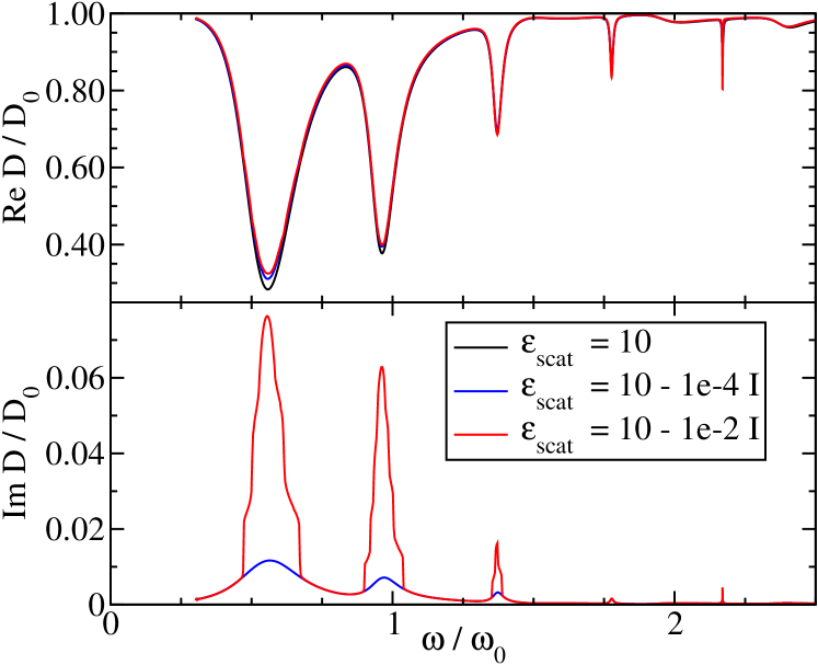
Figure 3: Normalized real part (upper panel) and imaginary part (lower panel) of the diffusion coefficient $D(\Omega=0)$ for different values of optical gain as indicated as a function of the dimensionless frequency. For the displayed frequency range, the gain value ist below threshold.

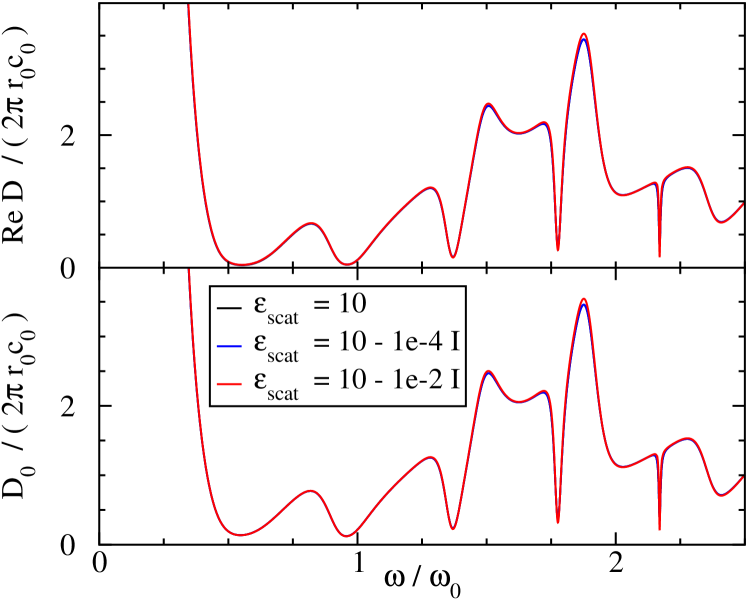
Figure 4: Real part of diffusion coefficient $D(0)$ (upper panel) and the bare diffusion coefficient $D_{0}$ (lower panel) for different values of the optical gain as a function of the dimensionless frequency. The diffusion coefficients are shown in natural units ($2\pi r_{0}c$), $r_{0}$ is the scatterers radius and c is the vacuum speed of light. The influence of optical gain on diffusion is seen to be small.

For completeness and later use we also display the bare diffusion constant $D_{0}$ and the real part of the full diffusion coefficient. The bare diffusion constant as shown in Fig. 4 exhibits strong variations as function of frequency but only small variation with increasing optical gain. The full diffusion coefficient in Fig. 4 follows closely the behavior of the bare diffusion, as already indicated in Fig. 3. For very small and also for large frequencies the difference is negligible, visible effects are found within an intermediate frequency range only.

III.2 Length and Time Scales

Within disordered systems there exist different length or time scales, related to both single and two-particle quantities. Additionally, a geometrical mean distance between each two scatterers $r_{m}$ can be defined by $\frac{r_{m}}{r_{0}}=\sqrt[3]{\frac{4\pi}{3\nu}}$, where $r_{0}$ is the scatterer’s radius and $\nu$ the filling fraction. For a filling fraction of $\nu=30\%$ this ratio becomes $\frac{r_{m}}{r_{0}}=2.41$.

The most important single particle length is the so-called scattering mean free path $l_{s}$ defined in the Green’s function

$$G_{\vec{q}}(\omega)=\frac{1}{\frac{\omega^{2}}{c^{2}}\epsilon_{0}-q^{2}-\Sigma(\omega)}$$ (35)

where the imaginary part of the self-energy introduces the decay length $l_{s}$

$$q = \frac{\omega}{c}\sqrt{\epsilon_{0}}\longrightarrow{\rm Re}(q)+\frac{i}{2l_{s}}$$ (36)

$$l_{s} = \frac{1}{2{\rm Im}(\sqrt{q^{2}+i{\rm Im}\Sigma(\omega)})}$$ (37)

The decay length may equivalently be represented as a life time of the corresponding k-mode.

In Fig. 6 the scattering mean free path is shown as a function of frequency. The strong variation with frequency is known to be typical for the low density approximation Tig92 ; Tig93 ; Bus95 as used in this publication. The minor dependence on gain is in agreement with the previous subsection and mainly established in slightly more pronounced dips and enhanced peaks.

Before proceeding, we want to emphasize that in case of real dielectric constants the scattering mean free path sets the scale determining the loss due to scattering out of a given k-mode. Whereas in case of gain media the originally k-mode experiences also an amplification. In this way a competition is established between scattering and gain. Once the optical gain is strong enough to compensate the scattering loss, i.e. ${\rm Im}\Sigma(\omega)=0$, that fact is interpreted as the crossing of the laser threshold Cao00 ; Cao03b ; cao05 ; Lagendijk_mie . This particular case consequently defines the range of validity of the presented theory, which cannot describe the onset of the laser dynamics. The gain coefficient is therefore to be chosen such that the system remains below its threshold gain value. This will be discussed in detail in subsection C below.

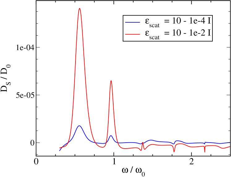
Figure 5: Normalized extra contribution to the diffusion coefficient $D_{s}/D_{0}$ for different values of the optical gain as a function of the dimensionless frequency.

Let us now return to the discussion of the intensity and the scales related to it. The two-particle Green’s function as given in Eq. (28 ) contains two obvious scales originating solely from finite values of the gain coefficient. These length scales may be defined by

$$\ell_{a}=\frac{2\pi}{{\rm Re}(\sqrt{1/\xi_{a}^{2}})}$$ (38)

$$\ell_{osc}=\frac{2\pi}{{\rm Im}(\sqrt{1/\xi_{a}^{2}})}$$ (39)

where $\ell_{a}$ represents the amplification or absorption length of the intensity and $\ell_{osc}$ marks the length over which the intensity oscillates, where $\xi_{a}^{2}$ has already been defined in Eq. (30 ). The corresponding time scales may then be defined as

$$\frac{1}{\tau_{a}} = \frac{D}{\xi_{a}^{2}}$$ (40)

$$\frac{1}{\tau_{osc}} = Q^{2}{\rm Im}D$$ (41)

The amplification or growth length $\ell_{a}$ is displayed in Fig. 7 as a function of the external light frequency. The single scatterer Mie resonances are clearly visible as well as strong dependence on the gain value. However, even for the strongest presented gain, the magnitude of the amplification length remains at least an order of magnitude larger than the corresponding scattering mean free path, shown in Fig. 6. Additionally, we have plotted the oscillation length $\ell_{osc}$ in Fig. 7. As compared to the amplification length the resonant character of the scattering is even more pronounced and $\ell_{osc}$ of course also strongly depends on the gain value. The magnitude is even significantly larger than the amplification length $\ell_{a}$. This fact may represent a large obstacle in experiments. The physical picture presents itself now as the following, if one measures the intensity distribution between two points in coordinate space in the sample at a given distance $r$, i.e. at a finite value of $Q$ in Eq. (28), one will measure a diffusive intensity decay as characterized by the real part of the diffusion constant plus an exponential amplification due to $\ell_{a}$ and additionally there is an amplitude modification proportional to $\cos(2\pi\ell_{a}/\ell_{osc})$ in case one chooses the measuring distance to be $\ell_{a}$. This means, in general even though the intensity has experienced an exponential increase by a factor of $e$, this oscillating modulation factor of the intensity is close to unity and therfore possibly hard to detect.

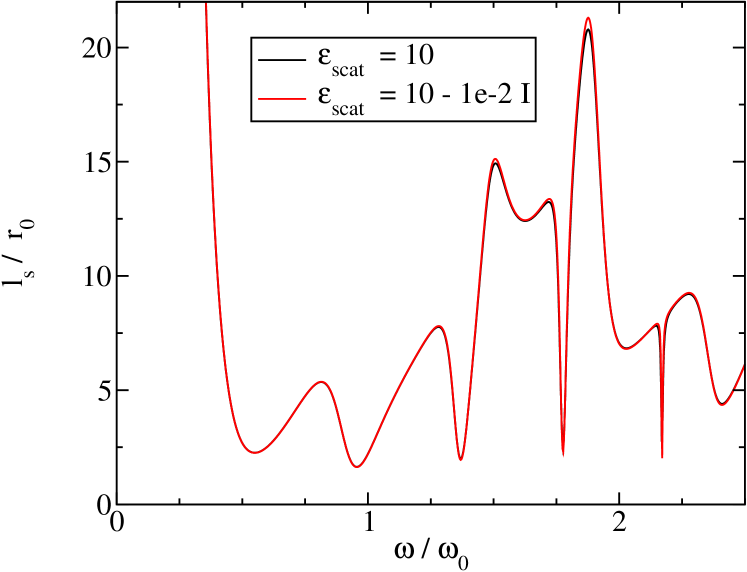
Figure 6: Displayed here is the single particle scattering mean free path $l_{s}$ for amplifying scatterers and conserving scatterers. The difference between the two is seen to be small and mainly manifests itself in narrow dips and peaks.

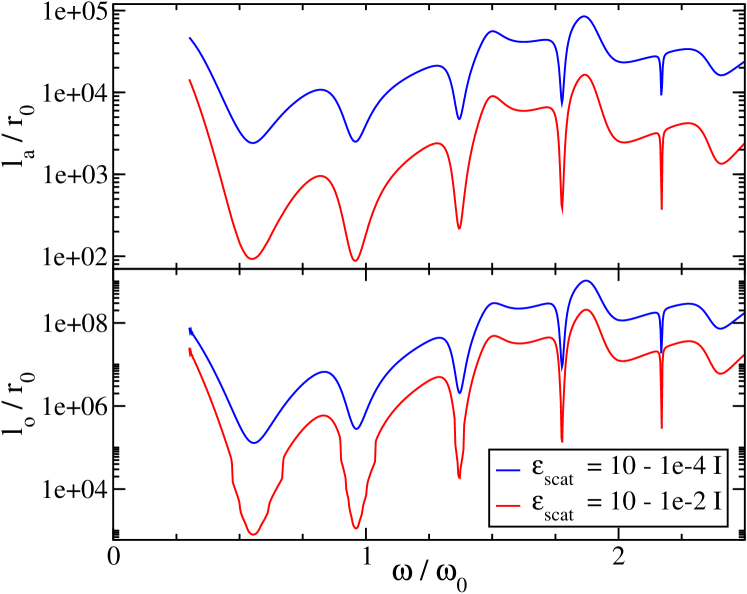
Figure 7: Displayed in the upper the two particle amplification length $l_{a}$ for different values of the optical gain as a function of the dimensionless frequency.
Displayed in the lower panel is the two particle oscillation length $l_{o}$ for different values of the optical gain as a function of the dimensionless frequency.

Slightly changing the point of view let us now turn to the time scales. In the upper panel of Fig. 8 we present the gain induced growth time $\tau_{a}$ defined in Eq. (40). For obvious reasons, $\tau_{a}$ displays a qualitatively similar behavior as the above discussed $\ell_{a}$, i.e., for frequencies within the scattering (Mie) resonances, the time to exponentially increase the intensity is significantly smaller than for frequencies outside this range. Which reflects the fact that the gain coefficient is confined to the scatterers volume only.

Using the gain induced growth rate $\tau_{a}$ as defined in Eq. (40), the intensity Green’s function Eq. (28 ) may now be rewritten as

$$P(Q,\Omega)=\frac{\alpha}{-i\Omega+iQ^{2}{\rm Im}D+Q^{2}{\rm Re}D-1/{\tau_{a}}}$$ (42)

where the coefficient $\alpha$ may symbolically contain all the factors explicitly shown and discussed in Eq. (28). By inspection of the above equation, Eq. (42) and comparison with the Green’s function Eq. (35), it is to be recognized that the energy density $P(Q,\Omega)$ also exhibits a laser-like threshold behavior in complete analogy to the single-particle Green’s function.

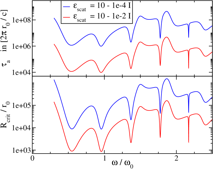
Figure 8: Displayed in the upper panel is the two particle amplification time $\tau_{a}$ for different values of the optical gain as a function of the dimensionless frequency.
In the lower panel we show the critical length $R_{crit}$, characterizing the threshold volume in which the intensity experiences a laser-like growth behavior.

Before discussing this threshold behavior in detail, we want to remind that our theory started with calculating the electrical field-field-correlator at different positions and frequencies Eq. (II.1) eventually leading to the evaluation the two particle Green’s function given in Eq. (28). This means, the momentum $Q$ appearing in Eq. (28) represents in Fourier space this relative position within the sample. In three dimensions the momentum $Q$ therefore defines a volume unit within the sample. This volume is carefully to be distinguished from all over length scales e.g. the sample volume etc. It is merely the volume within one considers correlation effects of the diffusing behavior of the intensity.

In analogy to ${\rm Im}\Sigma=0$ in the single particle Green’s function the threshold condition for the energy density now reads as follows

$$Q^{2}{\rm Re}D-1/{\tau_{a}} \geq 0$$ (43)

$$\Leftrightarrow\frac{4\pi^{2}}{R_{crit}^{2}}{\rm Re}D-1/{\tau_{a}} = 0$$ (44)

leading to the definition of a third, a critical, length scale

$$R_{crit}=2\pi\sqrt{\tau_{a}{\rm Re}D}.$$ (45)

This length describes the volume over which the energy density or intensity can compensate the diffusive loss by amplification due to the finite optical gain.

As in the above described case of a single particle Green’s function, the value $R_{crit}$ marks the point in parameter space where the laser threshold has been crossed. From the theoretically and experimentally known behavior of a lasing Mie sphere Lagendijk_mie ; Nussenzveig ; Vahala ; Lai and the theoretical description of the self-energy $\Sigma(\omega)$ by the single scatterer t-matrixTig92 ; Tig93 , and the definitions in Eq. (40) and Eq. (30) it becomes clear that in the limit of reaching the laser threshold within a Mie resonance $\tau_{a}$ is approaching zero, $\tau_{a}\rightarrow 0$. And therefore the corresponding critical volume of the light intensity becomes point-like. In situations where the optical gain is still below its threshold value with respect to the single scatterer Mie resonance, there is consequently a finite $\tau_{a}$ and therefore a finite critical volume described by $R_{crit}$. In the limit of large gain it becomes clear from the definitions in Eq. (40) and Eq. (38) that $R_{crit}$ in Eq. (45) approaches the same order of magnitude as $\ell_{a}$. Which is perfectly meaningful, since in this limit the smallest and all-dominant length scale is set by the amplification length. For the most interesting intermediate range, we show the critical length $R_{crit}$ in Fig. 8 as a function of light frequency for different gain strengths. Already for the gain values discussed in this publication, which are significantly below threshold, the ratio $R_{crit}/r_{0}$ becomes as small as approximately xxx, c.f. lower panels of Figs. 8 and 10.

Finally, we emphasize that, once a Mie resonance is close to lasing or the gain is very strong the growth time $\tau_{a}$ may become small and therefore the critical distance $R_{crit}$ may also become small as shown in the lower panel of Fig. 8. In general the length $R_{crit}$ is not restricted to values above e.g. the single particle scattering mean free path. This is because the underlying physics is not scattering but frequency independent amplification.

III.3 Gain and Laser Threshold

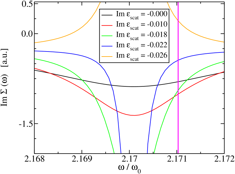
Figure 9: The imaginary part of the self-energy in the vicinity of the fifth Mie resonance for different but fixed values of gain. Increasing gain clearly yields narrowing and deepening until the laser threshold is reached, the curve approaches the shape of a delta-function. Beyond this point the theory is not valid anymore due to physical reasons. For completeness we also show the last curve ${\rm Im}\epsilon_{s}=-0.0026$ representing a system which has obviously crossed the threshold. The vertical line marks the frequency discussed in Fig. 10, see also text below.

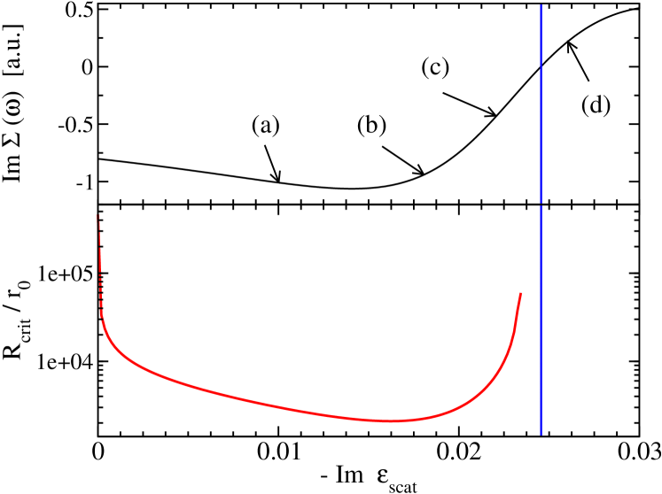
Figure 10: The upper panel shows the imaginary part of the self-energy at a fixed frequency ($\omega/\omega_{0}\simeq 2.1710269$) as a function of gain, c.f. Fig. 9. The vertical line signalizes the zero of ${\rm Im}\Sigma$. From Fig. 9 and the text below, it is clear that this zero indicated that the laser threshold has already been crossed. The points (a) through (d) correspond to $-{\rm Im}\epsilon_{scat}=\{0.01,0.018,0.022,0.026\}$, i.e. to the curves shown in Fig. 9. The intersections with the vertical line there yield the values shown here.
The lower panel displays the critical length $R_{\mbox{\tiny crit}}$ as a function of gain. Due to the off-resonant frequency, $R_{\mbox{\tiny crit}}$ has a local minimum and increases again with increasing gain.

In this last subsection, we want to closer discuss the appearance of a laser threshold within our theory. Since we approximate the single particle self-energy by the single particle scattering matrix calculated within Mie theory, we first recall some basic and well known facts. The resonant features representing the resonant scattering modes, arise due to poles in the scattering coefficients, forming the t-matrix. These poles, or zeros of the coefficients’ denominators, occur at complex frequencies, the closer the pole happens to be to the real frequency axes the more pronounced is the feature, i.e. the resonance becomes narrower and deeper. The effect of optical gain modeled as an imaginary part of the dielectric function, as it is done in this paper, is to lift the poles, i.e. it shifts the complex poles towards the real axes. In this way a gain narrowing is observed. The gain value corresponding to infinitesimal width of the resonance is believed to correspond to the experimentally observable laser threshold Lagendijk_mie . This situation coincides with a scattering pole right on the real frequency axes, i.e. the scattering resonance approaches the limiting shape of Dirac’s delta function with negative sign. Using gain values above threshold causes poles in the upper complex frequency half-plane, constituting unphysical behavior due to the neglected laser dynamics. If the complex frequency poles are in the upper half-plane, the theory still predicts a resonance feature, just with the ”wrong” sign, i.e. instead of dips in the retarded self-energy one now observes peaks, see also Fig. 9. Additionally the larger the gain, the less pronounced the feature becomes, because the poles are then pushed away from the real axes in the complex frequency plane. This contains the risk of utilizing much to high gain values, with poles in the negative complex frequency half-plane being at large distances to the real axes and therefore yielding very weak features that do not necessarily break causality of the single particle Green’s function for instance and might be overlooked at first glance.

To illustrate the above discussed subject in and out of resonance, we considered a system slightly off-resonant but close to the fifth Mie resonance as depicted in Figs. 9 and 10. In Fig. 9 the imaginary part of the self energy as a function of frequency is presented, the quantity describing both single particle scattering and amplification, as discussed earlier. For different gain values the narrowing and deepening of the resonance is clearly visible as well as the difference of systems below and above threshold. The vertical (magenta) line marks the single, off-resonant frequency for which we study the self-energy (upper panel) and the critical length $R_{crit}$ (lower panel) as a function of increasing gain, as shown in Fig. 10.

The behavior of ${\rm Im}\Sigma$ is easily understood by comparison with Fig. 9. It is to be noted that neither the local minimum nor the zero define the laser threshold. The behavior of $R_{crit}$ as defined in Eq. (45) is then shown in the lower panel of Fig. 10. The final increase is a consequence from the gain narrowing of the resonance. This decreases both the single particle scattering rate and the intensity emission rate $1/\tau_{a}$ defined in Eq. (40) and therefore increasing the critical volume. Following the above given line of arguments, it becomes clear that once a frequency closer to the resonance is chosen, the minimum value of $R_{crit}$ decreases because the scattering rate and the intensity emission rate both increase. Even for a finite spectral width of the resonance, i.e. for a system below threshold, the value of the critical length may become quite small.

IV Conclusion

In conclusion, we have presented a semi-analytical theory for scalar waves propagating in random, dissipating, i.e. also amplifying, media. The focus has been put on the influence of localization effects and finite gain on intensity transport in general. We found that for reasonable magnitudes of gain, the impact on transport quantities as e.g. the real part of the diffusion constant, scattering mean free path etc. is rather small. However, the gain introduces three new length scales natural to such systems, an amplification length $\ell_{a}$, an oscillation length $\ell_{osc}$ and a critical length $R_{crit}$. The latter describing the critical volume in which the intensity experiences a laser-like threshold behavior. The former two length scales constitute a growth length competing the diffusive loss of the intensity and the oscillation period of the intensity, respectively. Due to its comparably large magnitude, this oscillation length might be difficult to detect in experiments. We point out, that the critical length, or equivalently volume, has no lower bound other than zero since, e.g. for a Mie resonance reaching its lasing threshold this volume becomes point like. For cases below threshold gain within the Mie scatterers or off-resonant light, the critical volume is finite and strongly influenced by the gain coefficient.

Acknowledgments - The authors acknowledge for support the Karlsruhe School of Optics & Photonics (KSOP) (R.F.) and the SFB 608 (A.L.). For valuable discussions they want to thank Johann Kroha and Kurt Busch.

References

- (1) B.A. van Tiggelen, S.E. Skipetrov, Phys. Rev. E. 73, 045601 (2006) Rapid Communications
- (2) B.A. van Tiggelen, D. Anache and A. Ghysels, Europhys. Lett. 74, 999 (2006)
- (3) S. V. Zhukovsky, D. N. Chigrin, J. Kroha J. Opt. Soc. Am. B 23, 2265 (2006);
- (4) R. Frank, A. Lubatsch, and J. Kroha Phys. Rev. B 73, 245107 (2006); J. Opt. A: Pure Appl. Opt. 11, 114012 (2009).
- (5) M. Störzer, C. M. Aegerter, and G. Maret Phys. Rev. E 73, 065602 (2006)
- (6) M. Störzer, P. Gross, C. M. Aegerter, and G. Maret Phys. Rev. Lett. 96, 063904 (2006)
- (7) H. Cao, Waves in Random Media 13, R1 (2003).
- (8) K. L. van der Molen, P. Zijlstra, A. Lagendijk, A. P. Mosk Optics Letters 31, 1432, (2006)
- (9) A. Yamilov, X. Wu, X. Liu, R. P. H. Chang, and H. Cao Phys. Rev. Lett. 96, 083905 (2006)
- (10) Optics Letters, 30, 2430 (2005) A. Yamilov, X. Wu, H. Cao, A. L. Burin
- (11) Optics Letters, 29, 917 (2004) Shih-Hui Chang, Allen Taflove, Alexey Yamilov, Aleksander Burin, Hui Cao
- (12) P.W. Anderson, Phys. Rev. 109, 1492 (1958).
- (13) E. Abrahams P. W. Anderson, D. C. Licciardello, and T. V. Ramakrishnan Phys. Rev. Lett. 42, 673 (1979).
- (14) D. Vollhardt and P. Wölfle, Phys. Rev. Lett. 45, 842 (1980); Phys. Rev. Rev. B 22, 4666 (1980).
- (15) D.S. Wiersma , P. Bartolini, A. Lagendijk, and R. Righini, Nature 390, 671 (1997).
- (16) F. Scheffold , R. Lenke, R. Tweer, and G. Maret, Nature 398, 206 (1999).
- (17) D.S. Wiersma , J. Gomez Rivas, P. Bartolini, A. Lagendijk, and R. Righini, Nature 398, 207 (1999).
- (18) J.C.J. Paasschens, T.Sh. Misirpashaev, C.W.J. Beenakker Phys. Rev. B 54, 11887 (1996).
- (19) H. Cao , J. Y. Xu, D. Z. Zhang, S. H. Chang, S. T. Ho, E. W. Seelig, X. Liu, R. P. H. Chang, Phys. Rev. Lett. 84, 5584 (2000).
- (20) H. Cao, Y. Ling, J. Y. Xu, C. Q. Cao, and P. Kumar Phys. Rev. Lett. 86, 4524 (2001).
- (21) V.M. Apalkov, M.E. Raikh, B. Shapiro, Phys. Rev. Lett. 89, 016802 (2002).
- (22) H. M. Nussenzveig, J. Math. Phys. 10, 82 (1969).
- (23) K.J. Vahala, Nature 424, 839 (2003)
- (24) H. M. Lai, C. C. Lam, P. T. Leung, and K. Young, J. Opt. Soc. Am. B 8, 1962 (1991)
- (25) T. Kopp, J. Phys. C 17, 1897, 1918 (1984).
- (26) S. John, and M.J. Stephen, Phys. Rev. B 28, 6358 (1983).
- (27) J. Kroha, C.M. Soukoulis, and P. Wölfle, Phys. Rev. B 47, 11093 (1993).
- (28) Y. Kuga and J. Ishimaru, J. Opt. Soc. Am. B 1, 831 (1984).
- (29) M.P. van Albada and A. Lagendijk, Phys. Rev. Lett. 55, 2692 (1985).
- (30) P.E. Wolf and G. Maret, Phys. Rev. Lett. 55, 2696 (1985).
- (31) M.P. van Albada , B.A. van Tiggelen, A. Lagendijk, and A. Tip, Phys. Rev. Lett. 66, 3132 (1991).
- (32) B.A. van Tiggelen , A. Lagendijk, M.P. van Albada, and A. Tip, Phys. Rev. B 45, 12233 (1992).
- (33) B.A. van Tiggelen, A. Lagendijk, A. Tip, Phys. Rev. Lett. 71, 1284 (1993).
- (34) K. Busch and C.M. Soukoulis, Phys. Rev. Lett. 75, 3442 (1995); Phys. Rev. B 54, 893 (1996).
- (35) J. Kroha, Physica A 167, 231 (1990).
- (36) A. Lubatsch, J. Kroha, K. Busch, Phys. Rev. B 71, 184201 (2005).