Fractional Action Cosmology with Power Law Weight Function

Abstract

Motivated by an earlier work on fractional-action cosmology with a periodic weight function [1], we extend it by choosing a power-law weight function in the action. In this approach, we obtain a varying gravitational coupling constant. We then model dark energy in this paradigm and obtain relevant cosmological parameters.

1 Dirac’s Large Numbers Hypothesis and time running of $G$

During our survey of various physical laws of nature, we came across a number of constants entangled with these laws. Historically it was Weyl [2, 3] who initiated the idea of large numbers. However, it was Dirac who discovered an apparently unseen thread joining up these physical constants by a simple yet interesting law, viz., Law of Large Numbers. Using this law, Dirac arrived at his Large Number Hypothesis (LNH) which had profound influence on the world of physics. It generated a lot of activity both at theoretical and observational level with LNH as their starting point. Some works are centered around modification of Einstein’s gravitational theory and related equations to adapt the $G$ variation [4, 5]. Some authors have also given counter-arguments against LNH for justifying and refuting that hypothesis characterize the second category of works in favor of it [6] and also testing the validity of it [7]. Even there is found a formal link between LNH and cosmological constant term $\Lambda$ [8]. Weyl’s large number is square root of Eddington’s number $N\sim 10^{80}$ (which represents the total number of protons in the Universe) [9] and is supported by observational data [10]. Indeed Stewart showed that the ratio of the radius of the Universe and the electron is only two orders of magnitude smaller $10^{40}$ than that of Weyl s number. There are some other large numbers like Jordan’s number [11] and the Shemi-zadeh’s number [12] which have also appeared in the literature.

As originally stated by Dirac there are three dimensionless numbers in nature which can be constructed from the atomic and cosmological data:

1. The ratio of the electric to the gravitational force between an electron and a proton $\frac{e^{2}}{Gm_{e}m_{p}}\simeq 7\times 10^{39}$.

2. The mass of that part of the Universe that is receding from us with a velocity $v<c/2$ expressed in units of the proton mass is $10^{78}$.

3. The age of the Universe $t$, expressed in terms of a unit of time $\frac{e^{2}}{m_{e}c^{3}}$ provided by atomic constants, is inversely proportional to Newton’s gravitational constant.

The above three statements imply in respective order

$$\frac{e^{2}}{Gm_{e}m_{p}}\propto t,$$ (1)

$$M\propto t^{2},$$ (2)

$$G\propto t^{-1}.$$ (3)

There is a serious problem between (3) and GR [4, 13]: Einstein’s theory requires $G$ to be a constant. As was noted by Dirac, this inconsistency might be resolved if“.. we assume that Einstein theory is valid in a different system of units from those provided by the atomic constants.” Consequence of Dirac’s LNH is the existence of a variable $G$ cosmology. A beautiful account of the constants of nature appears in [14].

2 Framework

Recently Nabulsi [15] examined the Friedmann-Robertson-Walker (FRW) spacetime in the context of fractional action-like variational approach or fractionally differentiated Lagrangian function depending on a fractality parameter $\chi$ to model nonconservative and weak dissipative classical and quantum dynamical systems.

We apply the technical machinery of differential geometry to general relativity in the context of fractional action-like variational approach. Following Einstein’s arguments, we start by representing the gravitational field by an affine connection on a curved manifold and assume that the free fall corresponds to geodesic motion. Thus the classical Lagrangian of a curve is defined by $L=(1/2)g_{ij}\dot{x}^{i}\dot{x}^{j}$, where $\dot{x}^{i}=dx^{i}/dt$ and $g_{ij}$ is the metric tensor. This gives the action

$$S=\frac{m}{2}\int\limits_{0}^{\tau}g_{ij}(x)\dot{x}^{i}\dot{x}^{j}\mu(\chi,t)dt,$$ (4)

where $m$ is the particle’s mass. Here $\mu(\chi,t)$ is the generalized weight function and if we choose it to be a periodic function, we recover the results in [1]. This weight function can produce a friction force in classical dynamics for the test particle and as we will show, it also yields a time varying $G$. The modified resultant fractional Euler-Lagrange equations are

$$\ddot{x}^{l}+\partial_{t}\log(\mu(\chi,t))\dot{x}^{l}+\Gamma^{l}_{ij}\dot{x}^{i}\dot{x}^{j}=0.$$ (5)

We follow the procedure of [15] and assume that the test particle’s velocity is approximately zero. Furthermore, the metric and its derivative are approximately static. Applying these assumptions to the spatial components of (5) gives:

$$\partial_{i}\overrightarrow{\gamma}^{i}+\partial_{t}\mu\partial_{i}v^{i}+R_{tt}=0.$$ (6)

In the above equation $v^{i}=dx^{i}/dt$ and $\gamma^{i}=dv^{i}/dt$ are the particle’s velocity and acceleration respectively and $\partial_{i}\gamma^{i}=-4\pi G\rho$, which is Poisson’s equation in Newtonian gravity. Here $\rho$ is the mass density in gravitational interaction and $G$ is Newton’s gravitational constant. The resultant modified gravitational constant is

$$G^{\prime}=G\Big{(}1-\frac{\partial_{t}\log(\mu(\chi,t))}{4\pi G\rho}\partial_{i}v^{i}\Big{)}=G+\triangle G.$$ (7)

If $\mu(\chi,t)=t$ then (7) describes Dirac’s model [13]. Thus the change in $G$ in a spatially flat $(D+2)$-dimensional FRW Universe is

$$\triangle G=-\frac{D(D+1)H\partial_{t}\log(\mu(\chi,t))}{8\pi\rho},$$

where $H=\partial_{t}(\log(a(t))$ is the Hubble parameter. The Friedmann equation for such a model with metric $g_{ij}=diag(1,-a^{2}(t)\eta_{AB})$, $A,B=2,...,D+2,$ with $\eta_{AB}=diag(1,...,1)$ is

$$\frac{D(D+1)}{2}H^{2}=8\pi G\rho+\Lambda.$$ (8)

One thinks that if the gravitational constant changes slightly, as we have expressed it in this work, the Friedmann’s equation must be replaced by an effective $G$. A simple example of effective $G$ is the $f(R)$ gravity. An interesting feature of these theories is the fact that the gravitational constant is both time and scale dependent. After some calculations, one can obtain a Poisson equation in the Fourier space and attribute the extra terms as effective gravitational constant $G_{eff}$ [16]. But now, we are working using an Einstein-Hilbert action therefore there is no need to insert effective $G$ on the right hand side of the Friedmann’s equation (8).

Using the Bianchi identity and assuming both energy density $\rho$ and the cosmological constant $\Lambda$ as functions of time related by $\Lambda(t)=\Lambda_{0}\rho(t)^{n}$. Consequently we have

$$G(t)=\frac{G}{\mu(\chi,t)},\ \ \ \Lambda(t)=\Lambda_{n}\mu(\chi,t)^{n/(1-n)},\ \ \ \rho(t)=\rho_{n}\mu(\chi,t)^{1/(1-n)},$$ (9)

where $\Lambda_{n}\equiv\Lambda_{0}(\frac{8\pi G(1-n)}{\Lambda_{0}n})^{n/(n-1)}$ and $\rho_{n}\equiv(\frac{8\pi G(1-n)}{\Lambda_{0}n})^{1/(n-1)}$. Substituting (9) in (8) we obtain

$$H=\frac{\dot{a}}{a}=c_{n}\mu(\chi,t)^{n/(2(1-n))},$$ (10)

where $c_{n}=\sqrt{\frac{2b_{n}}{D(D+1)}}$ and $b_{n}=8\pi G\rho_{n}+\Lambda_{n}$ and $0<n<1$. By solving (10), we find

$$a(t)=a_{0}\exp\Big{(}c_{n}\int\mu(\chi,t)^{n/(2(1-n))}dt\Big{)}.$$ (11)

For the remaining part of the paper, we use power law weight function as

$$\mu(\chi,t)=\chi t^{p},\ \ \ \ p\geq 1.$$ (12)

One can treat (12) as a generalized Dirac’s hypothesis. Note that $p=1$ leads to an inverse power of time relation for the gravitational constant i.e. $G=\frac{G_{0}}{t}$. Substituting (12) in (11) yields

$$a(t)=a_{0}\exp(\alpha t^{\beta}),$$ (13)

where

$$\alpha\equiv\chi^{\frac{n}{2(1-n)}}\frac{2c_{n}(1-n)}{2+(p-2)n},\ \ \beta\equiv\frac{2+(p-2)n}{2(1-n)}.$$

It is useful to discuss the behavior of the scale factor diagrammatically. For simplicity we take $a_{0}=1$ and $\alpha=-1$, and focuss only on Dirac’s model i.e. $G(t)=\frac{G}{t}$. Figure 1 shows the behavior of the scale factor as a function of time for different values of $n$.

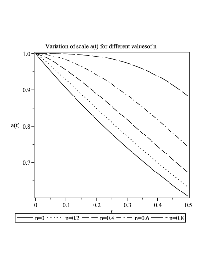
Figure 1: Variation of scale factor (13) for different values of $n$.

The Hubble parameter is

$$H=\alpha\beta t^{\beta-1}=\alpha\beta\Big{(}-\frac{1}{\alpha}\ln(1+z)\Big{)}^{1-\frac{1}{\beta}}.$$ (14)

Here redshift $z$ is defined by $1+z=\frac{a_{0}}{a(t)}$. Figure 2 shows the behavior of the Hubble parameter as a function of time for $\alpha=1$.

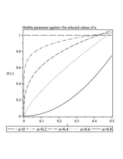
Figure 2: Hubble parameter against $t$ for selected values of $n$.

We note that the scale factor for $n=\frac{2}{3}$ , $\alpha=\frac{1}{2}$ is $a\propto\exp(\frac{t^{2}}{2})$. Consequently, the scale factor would increase very rapidly for the positive branch, while it would start from infinity for the negative branch. Also the choice $n=\frac{2}{3}$ , $\alpha=\frac{-1}{2}$ gives $a\propto\exp(\frac{-t^{2}}{2})$. This indicates that the Universe is evolving with a Hubble parameter $H\sim-t$ and a scale factor $a\propto\exp(\frac{-t^{2}}{2})$, which is close to singularity related to the origin and the fate of the Universe. The same phenomena occurs in the context of a new model of dark energy, the Quintom model [17].

2.1 Deceleration parameter

We know that

$$q=-1-\frac{\dot{H}}{H^{2}},$$ (15)

is the deceleration parameter. For an expanding Universe, $q>-1$. Using (14) we can write (16) as

$$q=-1-\frac{1-\beta}{\beta}\frac{1}{\ln(1+z)}.$$ (16)

For Dirac’s hypothesis ($p=1$), we have

$$q=-1+\frac{n}{2-n}\frac{1}{\ln(1+z)}.$$ (17)

Thus we conclude that the Universe can remain in an accelerating expansion for some values of $z$. The next diagram (Figure 3) represents the graph of $q$ versus $z$ for different values of $n$. It shows that when $n$ increases the deceleration parameter $q$ recedes from the crossing line $q=-1$ . Thus we can model cosmic acceleration in the present framework.

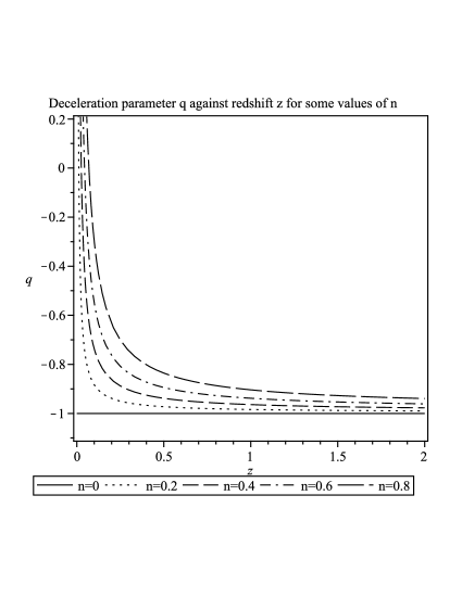
Figure 3: Deceleration parameter $q$ against redshift $z$ for some values of $n$.

2.2 The statefinder parameters for dark energy

The statefinder parameters $\{r,s\}$ were introduced to characterize primarily the spatially flat Universe ($k=0$) models with cold dark matter (dust) and dark energy [18]. They were defined as

$$r\equiv\frac{\ddot{a}}{aH^{3}}={\frac{\left({\beta}^{2}-3\,\beta+2\right){t}^{-2\,\beta}+\beta\,\left(\left(3\,\beta-3\right){t}^{-\beta}+\alpha\,\beta\right)\alpha}{{\alpha}^{2}{\beta}^{2}}},$$ (18)

$$s\equiv\frac{r-1}{3(q-\frac{1}{2})}=-\frac{2}{3}\,{\frac{\left(\beta-1\right)\left({t}^{-\beta}\beta-2\,{t}^{-\beta}+3\,\alpha\,\beta\right)}{\alpha\,\beta\,\left(3\,\alpha\,{t}^{\beta}\beta+2\,\beta-2\right)}}.$$ (19)

From (19) and (20) we obtain the relation between $r$ and $s$ as

$$r={\frac{{\alpha}^{2-\beta}\left(2+7\,s\beta\,y-4\,\beta-9\,s+16\,s\beta+2\,{s}^{2}{\beta}^{2}-13\,{s}^{2}\beta-7\,s{\beta}^{2}-7\,sy-2\,\beta\,y+2\,{\beta}^{2}+11\,{s}^{2}+2\,y\right)}{\left(-\beta+1-s\beta+s+y\right)^{2}}},$$ (20)

where

$$y=\sqrt{{\beta}^{2}-2\,\beta+2\,s\beta+1-2\,s+{s}^{2}{\beta}^{2}-2\,{s}^{2}\beta+{s}^{2}}.$$ (21)

We know that the cosmological constant possesses a fixed equation of state parameter $(w=-1)$ and a fixed Newton’s gravitational constant, hence $\{1,0\}$ corresponds to $\Lambda$CDM. Moreover $\{1,1\}$ represents the standard cold dark matter model containing no radiation while Einstein’s static Universe corresponds to $\{-\infty,\infty\}$ [19].

Note that for Dirac’s hypothesis $p=1,n=0,\beta=1$, we have $\{r,s\}=\{1,0\}$ which represents a static cosmological constant with cold dark matter. In Figure-4, we draw the pair $\{r,s\}$ for different values of $\beta=\frac{2-n}{2(1-n)},\alpha=1$. As we can see, the fixed gravitational constant occurs several times for some values of $n$. Also our model describes the standard cold dark matter and a static Einstein Universe for some values of $n$.

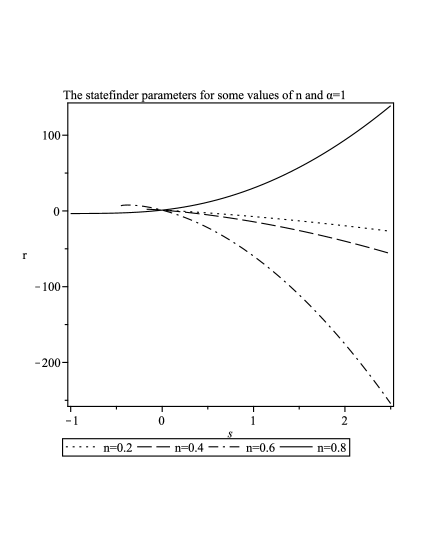
Figure 4: The statefinder parameters for some values of $n$.

2.3 Lookback time

If a photon is emitted by a source at the instant $t$ and received at time $t_{0}$, then the photon travel time or the lookback time $t-t_{0}$ is defined by

$$t-t_{0}=-\int_{0}^{z}\frac{dz}{H(z)(1+z)},$$ (22)

where $a_{0}$ is the present value of the scale factor of the Universe. It is appropriate to calculate this time as a function of $z$. After substituting Eq. (15) in Eq. (23) we have

$$t-t_{0}=-\frac{(-\alpha)^{1-1/\beta}}{\alpha\beta}\int_{0}^{z}\frac{dz}{(\log(1+z))^{1-1/\beta}(1+z)},$$

Now we change the variable as $x=\log(1+z)$. Calculating the integral above, we find

$$t-t_{0}=(-\frac{\log(1+z)}{\alpha})^{\frac{1}{\beta}}.$$ (23)

Figure-5 shows the behavior of the lookback time as a function of redshift for values $\alpha=-1,0<n<1$.

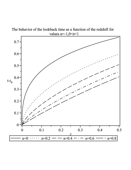
Figure 5: The behavior of the lookback time as a function of redshift for $\alpha=-1,0<n<1$.

2.4 Proper distance

If a photon is emitted by a source and is received by an observer at time $t_{0}$ then the proper distance between them is defined by

$$d=a_{0}\int_{a}^{a_{0}}\frac{da}{aH^{2}}=\int_{0}^{z}\frac{dz}{H^{2}(z)(1+z)}.$$ (24)

Using Eq. (15) in (25), we get

$$d=\frac{1}{\beta(\beta-2)}(-\frac{\ln(1+z)}{\alpha})^{-1+\frac{2}{\beta}}.$$ (25)

Figure 6 shows the behavior of proper distance in the present model.

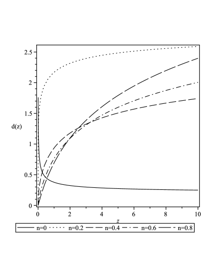
Figure 6: The behavior of the proper distance as a function of redshift for $\alpha=-1,0<n<1$.

2.5 Luminosity distance

If $L$ is the total energy emitted by the source per unit time and $\ell$ is the apparent luminosity of the object, then the luminosity distance $d_{L}=\left(\frac{L}{4\pi\ell}\right)^{\frac{1}{2}}$ evolves as

$$d_{L}=d(1+z)=\frac{z+1}{\beta(\beta-2)}\Big{(}-\frac{\ln(1+z)}{\alpha}\Big{)}^{-1+\frac{2}{\beta}}.$$ (26)

Figure (7) shows the variation of the luminosity distance as a function of the exponent $0<n<1$.

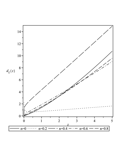
Figure 7: The behavior of the luminosity distance as a function of redshift for $\alpha=-1,0<n<1$.

2.6 Angular diameter

The angular diameter distance $d_{A}$ is

$$d_{A}=d_{L}(1+z)^{-2}=\frac{1}{\beta(\beta-2)(1+z)}(-\frac{\ln(1+z)}{\alpha})^{-1+\frac{2}{\beta}}.$$ (27)

Figure-8 shows the variation of the angular diameter as a function of the exponent $0<n<1$.

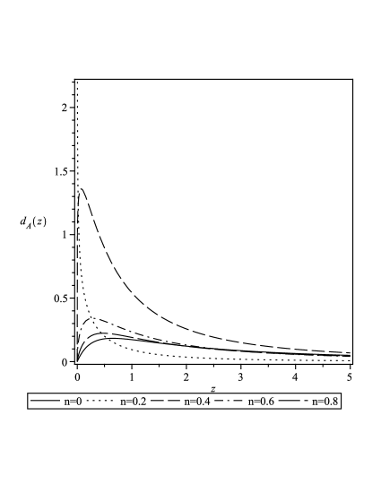
Figure 8: The behavior of the angular diameter as a function of redshift for $\alpha=-1,0<n<1$.

2.7 State parameter of dark energy

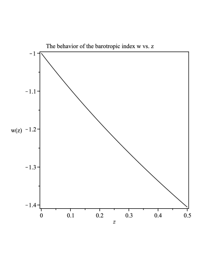
Figure 9: The behavior of the barotopic index $w$ vs. $z$

In this subsection we discuss the dynamics of the dark energy. We know that in a flat FRW model with a perfect fluid of pressure $p$ and energy density $\rho$, the barotropic index $w(t)$ is defined by

$$w(t)=-1-\frac{\partial_{t}\ln(\rho(t))}{3H},$$ (28)

which can be can be derived from the continuity equation. Using (9),(10) with (29) we obtain:

$$w(t)=-1-\frac{1}{3\left(-1+n\right)c_{{n}}}\,np{\chi}^{\,{\frac{n}{2(-1+n)}}}{t}^{\,{\frac{pn+2-2\,n}{2(-1+n)}}}.$$ (29)

For simplicity we take $D=2$, $\chi<<1$ and $G=\frac{1}{8\pi}$. Like the previous sections, we are interested in expressing $w$ as a function of $z$. We substitute $\beta=\frac{2+(p-2)n}{2(1-n)}$ and from Eqs. (24) and (30) we have

$$w(t) = -1-\frac{1}{3\left(-1+n\right)c_{{n}}}\,np{\chi}^{\,{\frac{n}{2(-1+n)}}}{\Big{(}\Big{[}\frac{-\log(1+z)}{\alpha}\Big{]}^{\frac{1}{\beta}}}\Big{)}^{\,{\frac{pn+2-2\,n}{2(-1+n)}}}.$$

Since $\frac{1}{\beta}\times\frac{pn+2-2n}{2(1-n)}=1$, therefore the previous equation reads

$$w(t) = -1+\frac{1}{3\alpha\left(-1+n\right)c_{{n}}}\,np{\chi}^{\,{\frac{n}{2(1-n)}}}\log(1+z),$$

Now using the values of $\rho_{n}$, $b_{n}$, $c_{n}$ and $\Lambda_{n}$, we can write

$$w(z)=-1-d_{{n}}\ln\left(1+z\right),$$ (30)

where

$$d_{n}=\frac{2p}{\sqrt{3}}(\frac{n^{n}\chi^{2-n}}{\Lambda_{0}(1-n)})^{\frac{1}{2(1-n)}}.$$ (31)

Also we observe from the previous figures, the model parameters do not depend on $p$ significantly and since the fractal parameter $\chi<<1$ therefore we limited ourselves only to $p=1$. From (30) it is obvious that the barotropic index crosses the dark energy limit $w(t)=-1$ for current era $z=0$ several times for different values of $\chi$ and $n$. For instance, using typical values $\chi=0.05,n=0.5,\Lambda_{0}=.01826$, (30) becomes

$$w(t)=-1-\ln\left(1+z\right).$$ (32)

Figure-9 shows the behavior of the barotopic index $w$ against $z$. The pressure may be written as

$$p(z)=-p_{n}(\ln(1+z)+d_{n}\ln(1+z)^{\frac{2-n}{n}}),$$ (33)

where

$$p_{n}=\rho_{n}\Big{(}-\frac{\chi}{\alpha}\Big{)}^{\frac{1}{1-n}}.$$ (34)

2.8 Consistency of the model $G(t)=\frac{G}{t}$ with observational constraints

From observational data, as it was shown in [20], there is a secular decrease of the gravitational constant $G(t)$. This time rate of change is of order $\frac{\dot{G}}{G}=(-5.9\pm 4.4)\times 10^{-14}yr^{-1}$ which was obtained from planetary data analysis. Thus, in our treatment on fractional cosmology focusing on the model $G(t)=\frac{G}{t}$, we can accept it as a reasonable model in good agreement with observational constraints [21].

Final remarks

This work was motivated by a more recent work on fractional-action cosmology with a periodic weight function in the action [1] which we extended using a power-law weight function. By doing so we obtained a varying gravitational coupling constant and also a time varying cosmological constant. For both of these ‘constants’, we used different ansatz to analyze the behavior of other parameters. We also modeled dark energy in this paradigm and obtained relevant cosmological parameters including distance parameters and statefinder parameters. The former helps in determining the nature of dark energy while the latter one classify different dark energy candidates.

Acknowledgments

The authors would like to thank R. A. El-Nabulsi for useful comments and valuable suggestions during this work. Also, we thank E. Pitjeva for pointing the note on secular decrease of the gravitational constant $G(t)$. M. Jamil would like to thank NUST for providing support to present this work at the III Italian-Pakistani Workshop on Relativistic Astrophysics in Italy.

References

References

- [1] EL. Nabulsi R A 2010 Commun. Theor. Phys 54, 16.
- [2] Weyl H 1917 Ann. Phys. 54, 117.
- [3] Weyl H 1919 Ann. Phys. 59, 101.
- [4] Dirac P A M 1973 Proc. R. Soc. Lond. 333, 403.
- [5] Canuto V, Hsieh S H, Adams P J 1977 Phy. Rev. Lett. 39 8.
- [6] Bousso R 2000 JHEP 0011, 038.
- [7] Blake G M 1978 Mon. Not. R. Astron. Soc. 185, 399.
- [8] Peebles P J E, Ratra B 2003 Rev. Mod. Phys. 75, 559.
- [9] Eddington A 1931 Proc. Cam. Phil. Soc. 27 (1931)
- [10] Stewart J The Deadbeat Universe Lars Wahlin, Colutron research, Boulder, Colorado, chap. 8, pp 104 (1931).
- [11] Jordan P Die Herkunft der Sterne (Stuttgart : Wissenschaftliche Verllagsgesellschaft M.B.H., 1947)
- [12] Shemi-zadeh V E 2002 gr-qc/0206084.
- [13] Dirac P A M 1937 Nature 139, 323.
- [14] Barrow J D 2002 The Constants of Nature, (Pantheon Books, 2002).
- [15] El-Nabulsi A R 2007 Rommanian Rep. Phys. 59, 763.
- [16] De Felice A, Tsujikawa S 2010 Living Rev. Relativity 13 ,3.
- [17] Cai Y-F, Saridakis E N, Setare M R, Xia J-Q 2010 Phys. Rep. 493, 1.
- [18] Sahni V, Saini T D, Starobinsky A A, Alam U 2003 JETP Lett. 77, 201.
- [19] Jamil M, Debnath U 2011 Int. J. Theor. Phys. 50, 1602.
- [20] Pitjeva E V 2010 EPM ephemerides and relativity (in) Relativity in Fundamental Astronomy: Dynamics, Reference Frames and Data Analysis, Proceedings IAU Symposium No. 261, Klioner S A, Seidelmann P K, Soffel M H, (eds.) Cambridge University Press, Cambridge, pp. 170-178.
- [21] http://iau-comm4.jpl.nasa.gov/plan-eph-data/index.html