arxiv:1106.2967

Open/Closed Topological ${\mathbb{C}}{\mathbb{P}}^{1}$ Sigma Model Revisited

Shmuel Elitzur ^a, Yaron Oz ^b, Eliezer Rabinovici ^a and Johannes Walcher ^c

^a Racah Institute of Physics, The Hebrew University of Jerusalem, 91904, Israel
^b Raymond and Beverly Sackler School of Physics and Astronomy
Tel-Aviv University, Ramat-Aviv 69978, Israel
^c Department of Physics, CERN - Theory Division,
CH-1211 Geneva 23, Switzerland

We consider the topological sigma-model on Riemann surfaces with genus $g$ and $h$ holes, and target space ${\mathbb{C}}{\mathbb{P}}^{1}\cong S^{2}$. We calculate the correlation functions of bulk and boundary operators, and study the symmetries of the model and its most general deformation. We study the open/closed topological field theory (TFT) correspondence by summing up the boundaries. We argue that this summation can be understood as a renormalization of the closed TFT. We couple the model to topological gravity and derive constitutive relations between the correlation functions of bulk and boundary operators.

November 2011

1 Introduction

In the first quantized string theory one often considers a string moving in a given geometrical background. One then obtains S-matrix elements by adding up contributions of worldsheet calculations with different worldsheet genera. In order to obtain a target space picture, one suggests a certain effective Lagrangian defined on the world volume, which was the target space in the worldsheet formulation [1]. This candidate is validated by comparing the S-matrix elements it produces to those obtained from the worldsheet procedure. This straightforward procedure does not address various questions such as the uniqueness of the effective lagrangian and its worldvolume and topology. One is actually familiar with symmetries such as T-duality and dynamical principles such as holography, which reflect ambiguities of the effective Lagrangian. In this work, we study this issue in a very simple setup, which does allow one to obtain the exact worldsheet results. This is the case of topological theories of matter.

Topological field theories (TFTs) provide a simple framework to study open/closed duality properties of string theory. One class of TFTs are the topological $\sigma$-models [2]. In order to construct these models we start with a $(2,2)$ supersymmetric non-linear $\sigma$-model in two-dimensions. This is a theory of maps $\Phi$ from a two-dimensional worldsheet $\Sigma$ to a target space $X$, which is a Kahler manifold. The two-dimensional $(2,2)$ theory has a $U(1)\times U(1)$ R-symmetry. One can twist the theory by adding to the stress tensor of the theory a derivative a $U(1)$ R-current. There are two ways to do that, i.e. twisting with the vector symmetry $U(1)_{V}$ or twisting with the axial symmetry $U(1)_{A}$. The first leads to the topological A-model, while the second to the topological B-model [3]. Due to the axial anomaly, the B-model is well defined only when the target space is a Calabi-Yau manifold. We will consider the topological A-model.

After the twisting, the supersymmetry transformation becomes a transformation under a nilpotent operator $Q$. The action becomes

$$S\sim\int_{\Sigma}d^{2}z\{Q,\Lambda\}+t\int_{\Sigma}\Phi^{*}(K)\ ,$$ (1)

where $\Phi^{*}(K)$ is the pullback to the worldsheet of the target space Kahler two-form. We will normalize

$$\int_{\Sigma}\Phi^{*}(K)=n\ ,$$ (2)

where $n$ is an integer, the degree of the instanton. The path integral of the theory localizes on holomorphic maps, and the correlation functions of the model depend only on the cohomology class of the Kahler form $K$.

In this paper we will consider the topological sigma-model on Riemann surfaces with genus $g$ and $h$ holes, and target space ${\mathbb{C}}{\mathbb{P}}^{1}\cong S^{2}$. We calculate the correlations function of bulk and boundary operators, study their symmetries and the open/closed TFT correspondence. The open/closed topological ${\mathbb{C}}{\mathbb{P}}^{1}$ model has been studied several times in the past, in the context of open/closed topological string correspondence and otherwise. (The earliest study we are aware of is [6].)

The paper is organized as follows. We will begin in section 2 by reviewing the elementary TFT correlation functions of the model, following [2, 5]. In section 3, we present our solution of the model at higher worldsheet topologies. In section 4, we analyze the duality properties of our results. In section 5 we couple the ${\mathbb{C}}{\mathbb{P}}^{1}$ model to topological gravity and present a few steps towards a complete study of the model. In particular, we obtain the constitutive relations of the disk amplitude on the large (closed string) phase space. Section 6 is devoted to a discussion. Part of the results on matter TFTs in this paper have been presented in [7].

2 The computational scheme

We will denote by $\langle O_{1}...O_{n}\rangle_{g,h}$ the correlation function of the operators $O_{1},...O_{n}$ on a Riemann surface with genus $g$ and $h$ boundaries. In this section we will outline the computational scheme that we will use in order to calculate these correlation functions.

2.1 The sphere

Consider first the correlators on the sphere with no boundaries. There are two operators of the topological ${\mathbb{C}}{\mathbb{P}}^{1}$ $\sigma$-model, the identity operator, ${\bf 1}$, and the operator corresponding to the second cohomology class of the sphere, which we shall denote by $H$. It is represented by a $\delta$-function two-form on ${\mathbb{C}}{\mathbb{P}}^{1}\cong S^{2}$. On the worldsheet $H$ is a zero-form. We have [2]

$$\begin{split}\langle{\bf 1}\rangle_{0,0}&=0\\ \langle H\rangle_{0,0}&=1\\ \langle H^{2}\rangle_{0,0}&=0\\ \langle H^{3}\rangle_{0,0}&=\beta\ ,\end{split}$$ (3)

where $\beta=e^{-t}$ comes from the classical action of the ${\mathbb{C}}{\mathbb{P}}^{1}$ $\sigma$-model and is the contribution of one-instanton, i.e. a degree one holomorphic map from the worldsheet to the ${\mathbb{C}}{\mathbb{P}}^{1}$ target space. The one-point correlator of $H$ is constant since it gets contribution only from the constant map: we map the worldsheet two-sphere to the target space two-sphere with the point where $H$ is inserted on the worldsheet being mapped to a given point in the target space. The three-point correlator of $H$ gets contribution from a degree one holomorphic map: we map the three insertion points to three given points on the target space. From (3), one derives the non-trivial ring relation (OPE)

$$H^{2}=\beta{\bf 1}\ .$$ (4)

2.2 The disk

We now want to consider the ${\mathbb{C}}{\mathbb{P}}^{1}$ model with branes included in the background. As shown in [5], there are two possible branes that preserve topological invariance. Geometrically, both of them correspond to the equator of ${\mathbb{C}}{\mathbb{P}}^{1}$, viewed as the two-sphere. The two branes are distinguished by the value $\epsilon=\pm 1$ of a Wilson line.

We consider correlators on the disc, with boundary condition corresponding to one of the two branes. Both branes support, in addition to the identity (which we continue to denote by ${\bf 1}$), a boundary operator corresponding to the first cohomology class of the equator circle [5], and we will denote this operator by $E$. It is represented by a $\delta$-function one-form on the equator, and is a zero-form on the worldsheet. It is shown in [5] that

$$\begin{split}\langle{\bf 1}\rangle_{0,1}&=0\\ \langle E\rangle_{0,1}&=1\\ \langle H\rangle_{0,1}&=0\\ \langle E^{2}\rangle_{0,1}&=0\\ \langle E^{3}\rangle_{0,1}&=\epsilon\beta^{1/2}\\ \langle EH\rangle_{0,1}&=\epsilon\beta^{1/2}\ .\end{split}$$ (5)

Here, it is understood that $E$ will be inserted on the boundary, while $H$ is inserted in the bulk of the disc. The one-point correlator of $E$ on the disk is constant since it receives contribution only from the constant map: we map the disk worldsheet to the target space $S^{2}$, such that the boundary of the disk is mapped to the equator and the insertion point on the boundary of the disk is mapped to a given point on the equator. This holomorphic map is the constant map. The three-point correlator of $E$ receives contribution from the disk one-instanton (or half-instanton in the closed string sense), which is a degree one map from the disk to $S^{2}$, where the boundary of the disk is mapped to the equator. The three insertion points on the boundary of the disk are mapped to three points on the equator.

The equations (5) imply the non-trivial relation on the boundary

$$E^{2}=\epsilon\beta^{1/2}\ ,$$ (6)

as well as the important relation

$$H=E^{2}=\epsilon\beta^{1/2}{\bf 1}$$ (7)

between the bulk field $H$ and the boundary field $E^{2}$. In other words, when computing a correlator on a Riemann surface with boundary, an insertion of $H$ in the bulk is equivalent to inserting $E^{2}$ on the boundary (or equivalently, inserting $\epsilon\beta^{1/2}{\bf 1}$, in the bulk or on the boundary).

It is also important to note that there are no boundary condition changing operators between $\epsilon=+1$ and $\epsilon=-1$.

2.3 Axial R-charge

We assign axial R-charges to the operators

$$R[H]=2,~{}~{}~{}~{}R[E]=1\ .$$ (8)

In general, an amplitude $\langle H^{n}E^{m}\rangle_{g,h}$ will be proportional to $\beta^{k}$ if $k$ is an integer (without boundaries) or half-integer (with boundaries) satisfying

$$\sum_{i}R_{i}=2n+m=4k+2-2g-h\ .$$ (9)

If there is no such $k$ the amplitude vanishes.

Note that a $(g,h)$ amplitude will vanish if both boundary conditions appear at the boundaries of the surface. This is because there are no boundary condition changing operators. Therefore, we will choose $\epsilon$ equal for all boundaries and fix it. Moreover, the amplitude will vanish unless $E$ is inserted an odd number of times on each boundary.

2.4 Handle and boundary states

An important idea of [2], picked up in [4], is that the TFT correlation functions on Riemann surfaces of higher genus can be computed as correlation functions on the sphere with some additional insertions. This idea can be straightforwardly generalized to the present situation with boundaries.

Thus, we introduce a handle operator $W$, with defining property.

$$\langle{\cal O}\rangle_{g,h}=\langle W{\cal O}\rangle_{g-1,h}\ ,$$ (10)

i.e., it relates correlators on surfaces of different topology. One can compute $W$ at $g=1$ by degenerating the torus into a sphere. Here, the relations

$$\begin{split}\langle W\rangle_{0,0}&=\langle{\bf 1}\rangle_{1,0}=2\langle H\rangle_{0,0}=2\\ \langle WH\rangle_{0,0}&=\langle H\rangle_{1,0}=2\langle H^{2}\rangle_{0,0}=0\ ,\end{split}$$ (11)

imply

$$W=2H\ .$$ (12)

When considering surfaces with boundaries, we have to fix boundary conditions $a_{1},a_{2},\ldots,a_{h}$ on each of them. Moreover, we have to allow for a dependence of the boundary state on the boundary insertions. We will then label the boundary states as $V_{a,\theta}$ to indicate dependence on the boundary condition and the boundary insertion. It satisfies

$$\langle{\cal O}\theta_{1}\cdots\theta_{h}\rangle_{g,h}=\langle{\cal O}\theta_{1}\cdots\theta_{h-1}V_{a_{h},\theta_{h}}\rangle_{g,h-1}\ .$$ (13)

It should be understood that the operator $\theta_{i}$ is inserted on the $i$-th boundary on the left and on the right hand side of the equation.

The boundary states can be computed on the disc. From (5), we learn

$$\begin{split}V_{\epsilon,{\bf 1}}&=0\\ V_{\epsilon,E}&=\epsilon\beta^{1/2}{\bf 1}+H\ .\end{split}$$ (14)

2.5 Frobenius algebra

Field theories can be axiomatized by the algebra structure provided by their operators. For a TFT on closed Riemann surfaces, the relevant structure is that of a Frobenius algebra (we consider the quantum algebra deformed by the worldsheet instantons). For the ${\mathbb{C}}{\mathbb{P}}^{1}$ model, the Frobenius algebra has a basis of idempotents, which are given by

$$H_{\pm}=\frac{1}{2}({\bf 1}\pm\beta^{-1/2}H)\ ,$$ (15)

and satisfy the algebra

$$H_{+}^{2}=H_{+}\qquad H_{-}^{2}=H_{-}\qquad H_{+}H_{-}=0\ .$$ (16)

The trace on the algebra is given by

$$\langle H_{\pm}\rangle_{0,0}=\eta_{\pm}\equiv\pm\frac{1}{2\beta^{1/2}}\ .$$ (17)

The handle operator is

$$W=\frac{H_{+}}{\eta_{+}}+\frac{H_{-}}{\eta_{-}}=2\beta^{1/2}(H_{+}-H_{-})\ .$$ (18)

Abstractly, branes should correspond to modules over the algebra of bulk operators, in other words, to (irreducible) representations of this algebra. Indeed, using (7), we learn that, in presence of the boundary $\epsilon$,

$$H_{\epsilon}={\bf 1}\qquad\qquad H_{-\epsilon}=0\ ,$$ (19)

which are indeed the possible representations of (16).

Note also that

$$V_{\epsilon,E}=2\epsilon\beta^{1/2}H_{\epsilon}=\frac{H_{\epsilon}}{\eta_{\epsilon}}\ .$$ (20)

3 Solving the ${\mathbb{C}}{\mathbb{P}}^{1}$ model

In this section we will compute the exact correlation functions of the ${\mathbb{C}}{\mathbb{P}}^{1}$ model. Here, by “exact”, we mean that we will sum over worldsheet topologies, but without coupling to topological gravity.

3.1 Summing over genera

We weight a closed Riemann surface of genus $g$ by a factor $\lambda_{c}^{2g-2}$, where $\lambda_{c}$ is the closed string coupling. Without boundaries we have [2, 4]

$$\begin{split}\langle\!\langle{\bf 1}\rangle\!\rangle&\equiv\sum_{g=0}^{\infty}\lambda^{2g-2}_{c}\langle{\bf 1}\rangle_{g,0}=\sum_{g=0}^{\infty}\lambda^{2g-2}_{c}\langle W^{g}\rangle_{0,0}=\sum_{g\text{ odd}}\lambda_{c}^{2g-2}\langle(2H)^{g}\rangle_{0,0}\\ &=\sum_{n=0}^{\infty}\lambda^{4n}_{c}2^{2n+1}\beta^{n}=\frac{2}{1-4\lambda^{4}_{c}\beta}\ ,\end{split}$$ (21)

and

$$\langle\!\langle H^{2s}\rangle\!\rangle = \sum_{n=0}^{\infty}\lambda^{4n}_{c}2^{2n+1}\beta^{n+s}=\frac{2\beta^{s}}{1-4\lambda^{4}_{c}\beta}\ ,$$

$$\langle\!\langle H^{2s+1}\rangle\!\rangle = \sum_{n=0}^{\infty}\lambda^{4n-2}_{c}2^{2n}\beta^{n+s}=\frac{\lambda_{c}^{-2}\beta^{s}}{1-4\lambda^{4}_{c}\beta}\ .$$ (22)

In the idempotent basis (16), this can be written as

$$\begin{split}\langle\!\langle H_{\epsilon}\rangle\!\rangle&=\sum_{g=0}^{\infty}\lambda^{2g-2}_{c}\langle H_{\epsilon}W^{g}\rangle_{0,0}=\sum_{g=0}^{\infty}\lambda^{2g-2}_{c}\eta_{\epsilon}^{1-g}=\frac{\lambda^{-2}_{c}\eta_{\epsilon}}{1-\lambda^{2}_{c}\eta_{\epsilon}^{-1}}\\ &=\frac{1}{\frac{\lambda^{2}_{c}}{\eta_{\epsilon}}\bigl{(}1-\frac{\lambda^{2}_{c}}{\eta_{\epsilon}}\bigr{)}}\ .\end{split}$$ (23)

This result is seemingly invariant under [4]

$$\frac{\lambda^{2}_{c}}{\eta_{\pm}}\leftrightarrow 1-\frac{\lambda^{2}_{c}}{\eta_{\pm}}\ .$$ (24)

Note, however, that according to (17), $\eta_{+}=-\eta_{-}$ and the transformations (24) are not mutually compatible. Thus, only correlators of one type, say $\langle\!\langle H_{+}\rangle\!\rangle$ are invariant and, in particular, $\langle\!\langle{\bf 1}\rangle\!\rangle$ is not invariant as can be easily checked. One can, however, deform the theory as to make it completely invariant. On general grounds, one expects the theory to depend on as many parameters as there are operators in the theory. As explained in [4], these parameters are most easily encoded in the sphere one-point functions of the basis of idempotents, while keeping fixed the rest of the OPE. In our case, we write

$$\langle H_{+}\rangle_{0,0}=\tilde{\eta}_{+}\,,\qquad\langle H_{-}\rangle_{0,0}=\tilde{\eta}_{-}$$ (25)

and we may in general treat $\tilde{\eta}_{-}$ as independent from $\tilde{\eta}_{+}$. We recover the standard ${\mathbb{C}}{\mathbb{P}}^{1}$ model on the subspace $\tilde{\eta}_{-}=-\tilde{\eta}_{+}$. Note that this deformation may or may not be realized in the standard BRST procedure, and may not survive coupling to topological gravity.

Now repeating the above computation we have

$$\langle\!\langle H_{\epsilon}\rangle\!\rangle=\frac{1}{\frac{\lambda^{2}_{c}}{\tilde{\eta}_{\epsilon}}\bigl{(}1-\frac{\lambda^{2}_{c}}{\tilde{\eta}_{\epsilon}}\bigr{)}}\ .$$ (26)

Since now $\tilde{\eta}_{+}$ and $\tilde{\eta}_{-}$ are independent parameters, we have an exact symmetry of the theory generated by

$$\frac{\lambda^{2}_{c}}{\tilde{\eta}_{\epsilon}}\rightarrow\frac{\lambda^{2}_{c}}{\tilde{\eta}_{\epsilon}},~{}~{}~{}~{}\frac{\lambda^{2}_{c}}{\tilde{\eta}_{-\epsilon}}\leftrightarrow 1-\frac{\lambda^{2}_{c}}{\tilde{\eta}_{-\epsilon}}\ .$$ (27)

Note that although we seem to have introduced three parameters $(\tilde{\eta}_{+},\tilde{\eta}_{-},\lambda)$, the correlation functions on closed Riemann surfaces depend only on two parameters, which are the combinations $(\frac{\lambda^{2}_{c}}{\tilde{\eta}_{\epsilon}},\epsilon=\pm)$.

3.2 The annulus

As a warmup for higher genus computations with background D-branes, let us check the factorization properties of the annulus correlator (see Fig. 1). We put equal boundary conditions on the two boundaries. There are then three amplitudes to consider: ${\bf 1}$ inserted on both boundaries, ${\bf 1}$ on one, $E$ on the other boundary, or $E$ on both boundaries.

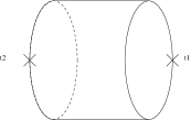
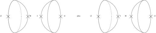
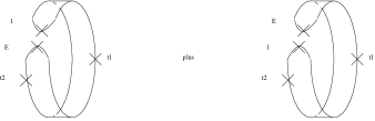
Figure 1: Factorizing the annulus

Factorizing via boundary states (middle of Fig. 1), we find

$$\begin{split}\langle{\bf 1}{\bf 1}\rangle_{0,2}&=0\\ \langle{\bf 1}E\rangle_{0,2}&=0\\ \langle EE\rangle_{0,2}&=2\epsilon\beta^{1/2}\ .\end{split}$$ (28)

We can also factorize as in the bottom of Fig. 1.

$$\langle{\bf 1}{\bf 1}\rangle_{0,2}=\langle{\bf 1}E\rangle_{0,1}\pm\langle E{\bf 1}\rangle_{0,1}\ ,$$ (29)

where $\pm$ is a sign that appears to be not so well understood in the general axiomatics of open-closed TFT (see,e.g., [8]). To be consistent, we here need this sign to be $-$. The second correlator

$$\langle{\bf 1}E\rangle_{0,2}=\langle{\bf 1}E^{2}\rangle_{0,1}\pm\langle E{\bf 1}E\rangle_{0,1}=0$$ (30)

does not suffer from this ambiguity and is consistent with (28) in any case. On the other hand,

$$\langle EE\rangle_{0,2}=\langle E^{3}\rangle_{0,1}\pm\langle E^{3}\rangle_{0,1}$$ (31)

requires $\pm=+$, in which case, using (5), we obtain agreement with (28). We conclude that the relative sign between the two terms in the last line of Fig. 1 depends on the boundary insertions.

3.3 General amplitudes

We now turn to a computation of exact correlation functions in the presence of background D-branes. In order to carry out this computation, we have to supply the combinatorial factors involved in summing over boundaries, and in distributing boundary insertions over the various boundaries. To remain flexible, we introduce an open string coupling constant $\lambda_{o}$ and weigh a worldsheet of topology $(g,h)$ by $\lambda_{c}^{2g-2}\lambda_{o}^{h}$. Our aim is to evaluate

$$\langle\!\langle E^{m}H^{n}_{\epsilon}\rangle\!\rangle\sim\sum_{g=0,h=1}^{\infty}\lambda_{c}^{2g-2}\lambda_{o}^{h}\langle E^{m}H^{n}_{\epsilon}\rangle_{g,h}\ ,$$ (32)

where we have written $\sim$ for the time being since we have not yet specified the combinatorial factors on the RHS.

Using the above handle and boundary operators, we find

$$\langle E^{m}H_{\epsilon}^{n}\rangle_{g,h}=\langle E^{m}H_{\epsilon}^{n}W^{g}\rangle_{0,h}=\eta_{\epsilon}^{-g}\langle E^{m}H_{\epsilon}\rangle_{0,h}\ ,$$ (33)

where we use $H_{\epsilon}^{2}=H_{\epsilon}$ and $W=H_{+}/\eta_{+}+H_{-}/\eta_{-}$, and we assume that all the boundaries carry label $\epsilon$. (As mentioned before, the amplitudes otherwise vanish.)

Note that to proceed with (33) we have to know how the boundary insertions are distributed on the various boundaries. This is not specified in (32), which involves a sum over all possible numbers of boundaries. Thus, there is an ambiguity that will accompany us for the next few pages. To ensure that (33) is non-vanishing, we assume $h\equiv m\bmod 2$, split the $m$ factors of $E$ into a group of $h$, to be put one on each boundary, and the remaining $s=(m-h)/2$ pairs into $h$ groups of arbitrary size.

Assuming the $E$’s are initially indistinguishable, this introduces a combinatorial factor of

$$\binom{s+h-1}{h-1}$$ (34)

so that we get:

$$\langle E^{m}H_{\epsilon}^{n}\rangle_{g,h}=\binom{s+h-1}{h-1}\eta_{\epsilon}^{-g}\bigl{(}2\eta_{\epsilon}\bigr{)}^{-s}(\eta_{\epsilon})^{-h}\eta_{\epsilon}\ ,$$ (35)

where we use $E^{2}=(2\eta_{\epsilon})^{-1}$, the boundary state $V_{\epsilon,E}=H_{\epsilon}/\eta_{\epsilon}$ as well as $\langle H_{\epsilon}\rangle_{0,0}=\eta_{\epsilon}$.

Now the sum over $h$ in (32) is restricted to those $h$ with the same parity as $m$. As above, we write $m=2s+h$, and sum over $s$. This yields

$$\langle\!\langle E^{m}H^{n}_{\epsilon}\rangle\!\rangle = \sum_{g=0}^{\infty}\sum_{s=0}^{m/2}\lambda_{c}^{2g-2}\lambda_{o}^{m-2s}\eta_{\epsilon}^{1-g+s-m}2^{-s}\binom{m-s-1}{m-2s-1}$$ (36)

$$= \frac{1}{\frac{\lambda_{c}^{2}}{\eta_{\epsilon}}\bigl{(}1-\frac{\lambda_{c}^{2}}{\eta_{\epsilon}}\bigr{)}}\sum_{s=0}^{m/2}\lambda_{o}^{m-2s}\eta_{\epsilon}^{s-m}2^{-s}\binom{m-s-1}{m-2s-1}\ .$$

The last sum in this expression is a certain hypergeometric polynomial. In order to check whether the symmetry (27) remains in the presence of boundaries, it is useful to compute $\langle\!\langle E^{m}H_{\epsilon}\rangle\!\rangle$ in the general deformation (25) We get in a straightforward fashion:

$$\langle\!\langle E^{m}H^{n}_{\epsilon}\rangle\!\rangle==\frac{1}{\frac{\lambda_{c}^{2}}{\tilde{\eta}_{\epsilon}}\bigl{(}1-\frac{\lambda_{c}^{2}}{\tilde{\eta}_{\epsilon}}\bigr{)}}\sum_{s=0}^{m/2}\lambda_{o}^{m-2s}\tilde{\eta}_{\epsilon}^{s-m}2^{-s}\binom{m-s-1}{m-2s-1}\ .$$ (37)

We can rescale the boundary operator by $E\rightarrow(2\eta_{\epsilon})^{\frac{1}{2}}E$. We then see that although we have introduced four parameters $(\tilde{\eta}_{+},\tilde{\eta}_{-},\lambda_{c},\lambda_{o})$ for the open plus closed system, the correlation functions in the presence of boundaries depend only on two parameters $(\frac{\lambda^{2}_{c}}{\tilde{\eta_{\epsilon}}},\frac{\lambda_{o}^{2}}{\tilde{\eta}_{\epsilon}})$ (for fixed choice of $\epsilon$). Note that in the presence of boundaries both signs of $\epsilon$ are not allowed simultaneously. It is then obvious the symmetry (27) of the closed TFT is preserved by the open plus closed system, provided we require that we keep $\frac{\lambda_{o}^{2}}{\tilde{\eta}_{\epsilon}}$ invariant. This works, whether or not we relate the open string coupling to the closed coupling, such as implied by unitarity in string theory. On the other hand, we do not see any new duality appearing in the open string sector. It is interesting to note that the sum over boundaries is less singular (a polynomial) than the sum over genera, which gives a pole at $\frac{\lambda_{c}^{2}}{\tilde{\eta}_{\epsilon}}=1$. This may be interpreted as an analogue of the fact that standard closed string (gravity) perturbation theory is more singular than open string (gauge theory) perturbation theory. In string theory, this distinction arises because of the properties of the moduli space of Riemann surfaces after coupling to worldsheet gravity, which we have not done.

4 Open/Closed duality

A way to view open/closed string theory duality is that summing up the open string degrees of freedom results in modifying the closed string background. Schematically,

$$\sum_{open}{\cal F}_{open+closed}(t_{o},t_{c})={\cal F}_{closed}(t^{\prime}_{c})\ .$$ (38)

Here $t_{o}$ and $t_{c}$ denote all the open and closed string moduli, and $t^{\prime}_{c}$ are the modified closed string moduli due to the open strings back reaction. A natural question is whether we can see such a duality in our open/closed topological field theory. We will see that in the absence of worldsheet gravity, summing up the open string degrees of freedom results in a renormalization of the closed TFT operator.

4.1 Generating Functionals

The generating functional $F_{g,h}(t_{H},t_{E})$ for the correlators of the type $\langle E^{m}H_{\epsilon}^{n}\rangle_{g,h}$ is characterized by the property

$$\frac{\partial^{n+m}F_{g,h}(t_{H},t_{E})}{\partial^{n}t_{H_{\epsilon}}\partial^{m}t_{E}}|_{t_{H}=0,t_{E}=0}=\langle E^{m}H_{\epsilon}^{n}\rangle_{g,h}\ .$$ (39)

As noted before, $H_{\epsilon}$ is defined with the same $\epsilon$ as the D-brane boundary condition. There are also the observables $H_{-\epsilon}$. However, correlators $H_{-\epsilon}$ with the other observables have only the disconnected parts. Define

$$\begin{split}{\cal F}_{open+closed}(\lambda_{c},\lambda_{o},t_{H},t_{E},\eta_{\pm})&=\sum_{g=0}^{\infty}\sum_{h=0}^{\infty}\lambda_{c}^{2g-2}\lambda_{o}^{h}F_{g,h}(t_{H},t_{E},\eta_{\pm})\\ &=\sum_{m=0}^{\infty}\sum_{n=0}^{\infty}\langle\!\langle E^{m}H_{\epsilon}^{n}\rangle\!\rangle\frac{t_{E}^{m}}{m!}\frac{t_{H_{\epsilon}}^{n}}{n!}\ .\end{split}$$ (40)

The generating functional for the correlators of the closed topological $\sigma$-model reads

$${\cal F}_{closed}(\lambda_{c},t_{H_{\epsilon}})=\frac{\frac{\eta_{\epsilon}}{\lambda_{c}^{2}}}{1-\frac{\lambda_{c}^{2}}{\eta_{\epsilon}}}\exp[t_{H_{\epsilon}}]\ .$$ (41)

In particular, using $\eta_{-\epsilon}=-\eta_{\epsilon}$ for the undeformed topological $\sigma$-model, we see that

$$\langle{\bf{1}}\rangle_{Exact}=\langle H_{\epsilon}+H_{-\epsilon}\rangle_{Exact}=\frac{2}{1-\Big{(}\frac{\lambda_{c}^{2}}{\eta_{\epsilon}}\Big{)}^{2}}\ .$$ (42)

We can obtain a simple expression for the closed generating functional after summing up over the boundaries. Recall that we can replace a boundary with an insertion of the boundary operator $E$ by using the operator $V_{\epsilon,E}$ as described by equations (13) and (14). We need to sum over the boundaries with any number of (odd) $E^{\prime}s$ inserted on each boundary. Consider first one boundary. We have

$$\lambda_{o}\sum_{m=1}^{\infty}\langle H_{\epsilon}E^{2m+1}\rangle_{0,1}\frac{t_{E}^{2m+1}}{(2m+1)!}=\langle H_{\epsilon}\rangle_{0,0}\lambda_{o}\Bigl{(}\frac{2}{\eta_{\epsilon}}\Bigr{)}^{1/2}\sinh\left[\frac{t_{E}}{(2\eta_{\epsilon})^{1/2}}\right]\ .$$ (43)

Now we need to sum over the number of boundaries, which exponentiates (43). This can be achieved in the generating functional by modifying

$$t_{H_{\epsilon}}\rightarrow\tilde{t}_{H_{\epsilon}}=t_{H_{\epsilon}}+\lambda_{o}\Bigl{(}\frac{2}{\eta_{\epsilon}}\Bigr{)}^{1/2}\sinh\left[\frac{t_{E}}{(2\eta_{\epsilon})^{1/2}}\right]\ .$$ (44)

Thus, the generating functional for the open plus closed topological $\sigma$-model (40) is obtained by using the change (44) in the generating functional of the closed topological $\sigma$-model (41). We see that summing up the open string degrees of freedom results in a renormalization of the closed string operator $H_{\epsilon}$ by adding to it an infinite series of the boundary operator $E$, weighted by $\eta_{\epsilon}$ and the open string coupling $\lambda_{o}$.

4.2 Alternatives

In this subsection, we explore some alternative combinatorial rules for summing over boundaries, in view of simplifying open-closed duality. To appreciate these alternatives, one has to realize that while the set of correlation functions satisfies the axioms of TFTs, we know of no a priori constraints on how to choose the combinatorial factors in summing over worldsheet topologies. This freedom is a consequence of the fact that we do not couple here the TFT to a worldsheet gravity. A related expectation is that eventually the ambiguities in summing the holes will be be removed by the uncovering of a new symmetry that should be maintained by the factors or by some other consistency argument. In the absence of this guiding principle we here advocate considering various possibilities mentioning each time an additional physical input, which would select that particular choice. We also include one choice, whose sole present motivation is the interesting result it implies on open-closed string duality. It displays a property consistent with our prejudices. The fact that other choices do not lead to that result should be kept as a cautionary fact as long as no new consistency conditions are uncovered.

As before, we assume the background of one D-brane labeled $\epsilon$, and use our formula (35) for the perturbative correlators. We now sum over genera, number of boundaries, and the number of bulk and boundary insertions. As before, we write $m=2s+h$. This leads to the full free energy:

$$\begin{split}F(\lambda_{c},\lambda_{0},t_{H_{\epsilon}},t_{E})&=\sum_{g,h,n,s}\frac{t_{H_{\epsilon}}^{n}}{n!}\,\frac{t_{E}^{2s+h}}{(2s+h)!}\,\lambda_{c}^{2g-2}\,\lambda_{o}^{h}\,\langle E^{2s+h}H_{\epsilon}^{n}\rangle_{g,h}\\ &=\sum_{g,h,n,s}\frac{t_{H_{\epsilon}}^{n}}{n!}\,\frac{t_{E}^{2s+h}}{(2s+h)!}\,\lambda_{c}^{2g-2}\,\lambda_{o}^{h}\,\frac{(s+h-1)!}{s!(h-1)!}\eta_{\epsilon}^{1-g-h-s}\\ &=\frac{\eta_{\epsilon}}{\lambda_{c}^{2}}\frac{1}{1-\frac{\lambda_{c}^{2}}{\eta_{\epsilon}}}\,{\rm e}^{t_{H_{\epsilon}}}\,\sum_{s,h}\frac{(s+h-1)!}{(2s+h)!s!(h-1)!}\lambda_{o}^{h}\eta_{\epsilon}^{-h-s}t_{E}^{2s+h}\ .\end{split}$$ (45)

The first factor is from geometric sum over genus. The second is the exponential factor from summing over bulk insertions. The last factor however is from devil’s kitchen, and cannot be done in a closed form. Note however that it does contain $1/(h-1)!$, which might be intuitively expected from indistinguishability of the boundaries.

We now invoke the right to modify the combinatorial factor involved in summing over boundary insertions. For example, we might consider replacing $t_{E}^{m}/m!$ with $t_{E}^{2s}/(2s)!$ if we decided not to count the first insertion that goes on each boundary to make the correlator non-zero. A physical way to justify this modification is to consider D-branes on which we have “turned on” the $E$ insertion. The mathematical advantage is that we are now able to do the sum:

$$\sum_{s,h}\frac{(s+h-1)!}{(2s)!s!(h-1)!}\left(\frac{\lambda_{o}}{\eta_{\epsilon}}\right)^{h}\,\left(\frac{t_{E}^{2}}{\eta_{\epsilon}}\right)^{s}=\frac{y}{1-y}\cosh\sqrt{\frac{x}{1-y}}\ ,$$ (46)

where $y=\lambda_{o}/\eta_{\epsilon}$, and $x=t_{E}^{2}/\eta_{\epsilon}$. So

$$F(\lambda_{c},\lambda_{0},t_{H_{\epsilon}},t_{E})=\frac{{\rm e}^{t_{H_{\epsilon}}}}{\frac{\lambda_{c}^{2}}{\eta_{\epsilon}}(1-\frac{\lambda_{c}^{2}}{\eta_{\epsilon}})}\;\frac{\frac{\lambda_{o}}{\eta_{\epsilon}}}{(1-\frac{\lambda_{o}}{\eta_{\epsilon}})}\cosh\tilde{t}_{E}\ ,$$ (47)

where $\tilde{t}_{E}=t_{E}\sqrt{\frac{\frac{1}{\eta_{\epsilon}}}{1-\frac{\lambda_{o}}{\eta_{\epsilon}}}}$. This result does not to allow an interpretation as an open-closed string duality, with a closed dual theory being a deformation of the original TFT. We are therefore encouraged to look for other possibilities.

Another possible proposal for the combinatorial factor is to claim that we should only count boundary insertions in pairs. This would mean putting $t_{E}^{s}/s!$ in the sum, which becomes

$$\sum_{s,h}\frac{(s+h-1)!}{s!s!(h-1)!}x^{s}y^{h}=\frac{y}{1-y}{\rm e}^{x/(1-y)}\ ,$$ (48)

with $y=\lambda_{o}/\eta_{\epsilon}$ as before and $x=t_{E}/\eta_{\epsilon}$. Then

$$F(\lambda_{c},\lambda_{o},t_{H_{\epsilon}},t_{E})=\frac{{\rm e}^{t_{H_{\epsilon}}}}{\frac{\lambda_{c}^{2}}{\eta_{\epsilon}}(1-\frac{\lambda_{c}^{2}}{\eta_{\epsilon}})}\;\frac{\frac{\lambda_{o}}{\eta_{\epsilon}}}{(1-\frac{\lambda_{o}}{\eta_{\epsilon}})}{\rm e}^{\tilde{t}_{E}}\ ,$$ (49)

with $\tilde{t}_{E}=t_{E}\frac{\frac{1}{\eta_{\epsilon}}}{1-\frac{\lambda_{o}}{\eta_{\epsilon}}}$. This result is quite similar to (47), without a manifest open-closed duality.

By way of answer analysis, one may check that in order to obtain a standard open-closed duality, we would need the combinatorial factor for summing over boundary insertions to be

$$\frac{t_{E}^{s}}{(s+h-1)!}$$ (50)

Then the sum becomes

$$\sum_{s,h}\frac{1}{s!(h-1)!}\left(\frac{\lambda_{o}}{\eta_{\epsilon}}\right)^{h}\;\left(\frac{t_{E}}{\eta_{\epsilon}}\right)^{s}=\frac{\lambda_{o}}{\eta_{\epsilon}}{\rm e}^{t_{E}/\eta_{\epsilon}}{\rm e}^{\lambda_{o}/\eta_{\epsilon}}\ .$$ (51)

In this scheme, the effect of integrating out the open strings is a shift of the closed string parameter

$$t_{\rm closed}\to t_{\rm closed}+\lambda_{o}/\eta_{\epsilon}\ .$$ (52)

Note, however, that we do not currently have a physical justification for (50). Also, the ${\rm e}^{t_{E}/\eta_{\epsilon}}$. term deserves a better understanding.

5 Coupling to Topological Gravity

In this section, we initiate a systematic attempt to couple the open-closed topological ${\mathbb{C}}{\mathbb{P}}^{1}$ model to topological gravity, starting from first principles (i.e., without using dualities of any sort). To the best of our knowledge, this has not been attempted before, mostly, it appears, because the notion of open topological gravity is severely under-developed, and naively mathematically ill-defined. (We believe, however, that a sensible version exists.) As in the previous sections, we here take a pragmatic approach, leaving justifications to future work. The key to success will be to consider only gravitational descendants in the bulk, and not on the boundary.

5.1 Topological gravity

When coupling the closed topological ${\mathbb{C}}{\mathbb{P}}^{1}$ $\sigma$-model to topological gravity, we have the following operators: In the closed sector we have the puncture operator $P$ that fixes a point in the bulk of the worldsheet (creates a puncture), and the primary operator $H$. In addition we have the gravitational descendants $\sigma_{k}(P),\sigma_{k}(H),k=1,2,...$.

When all couplings are turned off, we have the following non-vanishing correlators at genus $0$ [2]

$$\langle PPH\rangle_{0,0}=1\,,\qquad\langle H^{n}\rangle_{0,0}=1\,,\qquad\text{for all $n\geq 3$}\ .$$ (53)

The first equation is the contribution from the degree $0$ sector, and the second from sector with instanton number $1$. Note the difference to the correlators without coupling to topological gravity (3). Most succinctly, this change can be seen in the selection rule. Without coupling to topological gravity, this selection rule is

$$1+2k=n_{H}\ ,$$ (54)

where $n_{H}$ is the number of insertions of $H$, and $k$ is the instanton number (the degree of the map ${\mathbb{C}}{\mathbb{P}}^{1}\to{\mathbb{C}}{\mathbb{P}}^{1}$) Coupling to topological gravity modifies this to

$$-2+n_{P}+n_{H}+2k=n_{H}\ ,$$ (55)

where $n_{P}$ is number of insertions of puncture operator. Note that $n_{H}$ drops out of (55), whereas (54) does not depend on $n_{P}$.

Now note that in models such as ${\mathbb{C}}{\mathbb{P}}^{1}$, insertions of operators correspond to ordinary derivatives with respect to the corresponding couplings, e.g.,

$$\partial_{t_{0,H}}\langle\cdots\rangle=\langle H\cdots\rangle\,,\qquad\partial_{t_{0,P}}\langle\cdots\rangle=\langle P\cdots\rangle\ .$$ (56)

This implies that the relations (53) can be summarized in the following generating function (“prepotential”)

$$F^{(0,0)}=\langle\rangle_{0,0}=\frac{1}{2}t_{0,P}^{2}t_{0,H}+{\rm e}^{t_{0,H}}\ .$$ (57)

Equivalently, on the small phase space, we have the correlators

$$\begin{split}\langle PP\rangle_{0,0}&=t_{0,H}\\ \langle PH\rangle_{0,0}&=t_{0,P}\\ \langle HH\rangle_{0,0}&={\rm e}^{t_{0,H}}\end{split}$$ (58)

To study the large phase space (turn on coupling to descendants), it is a good idea to rewrite (58) as “constitutive relations”. Namely, as emphasized in [9], the functional form of the correlators is unchanged if we express them as functions of the coordinates

$$\begin{split}u^{P}&=\langle PP\rangle_{0,0}=t_{0,H}\\ u^{H}&=\langle PH\rangle_{0,0}=t_{0,P}\ .\end{split}$$ (59)

Using this, the constitutive relation of ${\mathbb{C}}{\mathbb{P}}^{1}$ is

$$\langle HH\rangle_{0,0}={\rm e}^{\langle PP\rangle_{0,0}}\ .$$ (60)

To show that (60) holds on the large phase space, it is enough to show that the derivatives with respect to the descendant couplings $t_{k,P}$ and $t_{k,H}$ vanish for $k\geq 1$. For this, let’s temporarily drop the $(0,0)$ subscript and consider

$$\partial_{t_{k,X}}\langle HH\rangle\overset{?}{=}\partial_{t_{k,X}}{\rm e}^{\langle PP\rangle}\ ,$$ (61)

where $X$ is $P$ or $H$, and we have turned on arbitrary values of all the couplings. Now

$$\begin{split}\partial_{t_{k,X}}\langle HH\rangle&=\langle\sigma_{k}(X)HH\rangle\\ &=k\langle\sigma_{k-1}(X)H\rangle\langle PHH\rangle+k\langle\sigma_{k-1}(X)P\rangle\langle HHH\rangle\\ &=k\langle\sigma_{k-1}(X)H\rangle\partial_{t_{0,P}}\langle HH\rangle+k\langle\sigma_{k-1}(X)P\rangle\partial_{t_{0,H}}\langle HH\rangle\ ,\end{split}$$ (62)

where we have used the topological recursion relations [2]. On the other hand

$$\begin{split}\partial_{t_{k,X}}{\rm e}^{\langle PP\rangle}&={\rm e}^{\langle PP\rangle}\langle\sigma_{k}(X)PP\rangle\\ &={\rm e}^{\langle PP\rangle}\Bigl{(}k\langle\sigma_{k-1}(X)H\rangle\langle PPP\rangle+k\langle\sigma_{k-1}(X)P\rangle\langle HPP\rangle\Bigr{)}\\ &=k\langle\sigma_{k-1}(X)H\rangle\partial_{t_{0,P}}{\rm e}^{\langle PP\rangle}+k\langle\sigma_{k-1}(X)H\rangle\partial_{t_{0,H}}{\rm e}^{\langle PP\rangle}\ .\end{split}$$ (63)

Now (62) and (63) together with (60) at $t_{k,P}=t_{k,H}=0$ imply that the constitutive relations (60) hold on the large phase space as well.

5.2 Adding boundaries

In the open sector we have the operator $B$ that fixes a point on the boundary of the worldsheet and the primary operator $E$. As we will argue, there are no gravitational descendants of the boundary primary operators.

Now let us add the A-brane wrapped on the equator of ${\mathbb{C}}{\mathbb{P}}^{1}$, with trivial gauge field, and consider the disk amplitude. Relevant instantons are now maps

$$(D,\partial D)\to({\mathbb{C}}{\mathbb{P}}^{1},{\mathbb{R}}{\mathbb{P}}^{1})\ .$$ (64)

Any such map can be complex conjugated to a map from ${\mathbb{C}}{\mathbb{P}}^{1}\to{\mathbb{C}}{\mathbb{P}}^{1}$, and we call the instanton number to be the ordinary degree of this doubled map. Note however that the requirement that the boundary of the disk map to the A-brane implies that the dimension of moduli space of such real maps is half of what it was in the complex case.

Before coupling to topological gravity, the selection rule is

$$1+2k=2n_{H}+m_{E}\ ,$$ (65)

where $m_{E}$ is the number of insertions of the boundary operator $E$. Note that (65) is an equality on real dimensions. After coupling to gravity, the selection rule becomes

$$-2+2k+2n_{H}+m_{E}+2n_{P}+m_{B}=2n_{H}+m_{E}\ .$$ (66)

Now let us try to write down some correlators of primaries, after coupling to topological gravity. First of all, the selection rule (66) allows only solutions for $k=0$ and $k=1$. From $k=0$, we find a non-vanishing correlator from $m_{B}=2$, $n_{P}=0$.

$$\langle BBE\rangle_{0,1}=1\ ,$$ (67)

which simply comes from the constant map to the point dual to $E$. Similarly, for $m_{B}=0$, $n_{P}=1$, we get

$$\langle PE\rangle_{0,1}=1\ .$$ (68)

However, any further insertion of $E$, or trying to insert $H$ instead of $E$, gives a vanishing result, because a constant map can only map to a single point. (Ultimately, this statement might require some rectification in view of (76) below.)

Now what about instanton sector 1, in which (66) implies we have no insertions of puncture operators? First, note that there are two maps in this sector: The map covering the northern half of the sphere, and the map covering the southern half of the sphere. Second, consider correlators with only boundary insertions. The first non-trivial one to consider is $\langle E^{3}\rangle$. Before coupling to gravity, only one of the two possible instantons contributed to this amplitude because of the fixing of the cyclic ordering of the boundary insertions. Specifically, in the topological sigma model before coupling to gravity, the amplitude is defined by

$$\langle E^{3}\rangle=\langle E(x_{1})E(x_{2})E(x_{3})\rangle\ ,$$ (69)

where the $x_{i}$ are some fixed insertion points on the boundary of the disk. Thinking of the latter as the upper half plane with boundary the real line, we can choose the three insertion points to be $x_{1}=0$, $x_{1}=1$, $x_{3}=\infty$. Now to compute (69), we choose three generic points $p_{1}$, $p_{2}$, $p_{3}$ on the A-brane (equator of ${\mathbb{C}}{\mathbb{P}}^{1}$), each representing the Poincaré dual of the cohomology class $E$ generating $H^{1}(S^{1},{\mathbb{Z}})$, and count the number of maps (instantons) mapping $x_{i}$ to $p_{i}$. It is not hard to see that depending on the cyclic ordering of $p_{1}$, $p_{2}$, $p_{3}$, such a degree one map has to cover either the northern or the southern hemisphere.

After coupling to topological gravity, the situation changes dramatically. The definition of the amplitude now involves an integration over the position of the insertion points, and dividing by the isometry group $SL(2,{\mathbb{R}})$ (in contrast, the definition of (69) a priori depends on $x_{1}$, $x_{2}$, $x_{3}$). Although the $SL(2,{\mathbb{R}})$ symmetry of the disk still allows us to fix the three insertion points at $0$, $1$, and $\infty$, we have to allow both possible cyclic orderings. Hence, both hemispheres contribute to the correlator. It us natural to assume that they contribute with opposite sign. (Justifying this requires a more careful study of orientation of the relevant moduli spaces from which we refrain here.) This implies that after coupling to topological gravity,

$$\langle E^{3}\rangle_{0,1}=0\ .$$ (70)

Continuing in this vein, we can add further boundary insertions. Each time, both hemispheres contribute because we can always arrange both required cyclic orderings of insertion points on the boundary of the disk. For an even number of insertions, the two come with the same sign, and for an odd number of insertions, we get a cancelation. (This is a consequence of the fermionic nature of $E$.) Thus

$$\langle E^{m}\rangle_{0,1}=1+(-1)^{m}\ .$$ (71)

Finally, we consider correlators with insertion of $H$. A seemingly simple correlator to compute is $\langle EH\rangle$. Naively, one chooses a point $p$ on the equator to represent $E$, and a point $q$ in the bulk to represent $H$. Using $SL(2,{\mathbb{R}})$ invariance to put insertion of $H$ at $z=0$ the center of the disk, and insertion of $E$ at say $x=1$ say, one looks for a map that maps the center of the disk to $q$ and $x=1$ on the boundary to $p$. There is a single such map in instanton sector $1$. It is the northern or southern hemisphere depending on where $q$ is chosen. So one might conclude naively

$$\langle EH\rangle_{0,1}=1\ .$$ (72)

We claim, however, that this equation, is wrong. To see this, imagine we wanted to compute $\langle EH^{2}\rangle_{0,1}$ by choosing a second bulk point $q^{\prime}$ to which we want to map a second bulk point $z^{\prime}$. Since the map was already fixed by $p$ and $q$, it boils down to the question of whether the second point $z^{\prime}$, in the interior of the disk (over which we are integrating) can be chosen such that it maps to $q^{\prime}$. The answer to this question now depends on whether we choose $q^{\prime}$ in the northern or southern hemisphere! But clearly, the amplitude cannot depend on the choice of representative for $H$, so something must be wrong with the reasoning leading to (72).

It is quite easy to see where the problem comes from on the worldsheet, which also suggests the resolution. What we are trying to do is insert

$$\int_{D}\Phi^{*}(\omega)$$ (73)

into the path integral and claim that it gives something well-defined if we think of $\omega$ as a cohomology class in $H^{2}({\mathbb{C}}{\mathbb{P}}^{1})$. But clearly if we change the representative $\omega\to\omega+d\psi$, (73) changes by a boundary term

$$\int_{D}\Phi^{*}(d\psi)=\int_{\partial D}\Phi^{*}(\psi)\ .$$ (74)

The well-known way to resolve this is to add explicit boundary term in the form of the Wilson line

$$\int_{\partial D}A\ .$$ (75)

Mathematically, speaking, we have to think of $\omega$ as a relative cohomology class in $H^{2}({\mathbb{C}}{\mathbb{P}}^{1},{\mathbb{R}}{\mathbb{P}}^{1})$. Thinking this through, we learn that the correct and invariant way to represent the operator $H$ is as the sum of a point in one of the hemispheres of ${\mathbb{C}}{\mathbb{P}}^{1}$ together with $1/2$ times a point on the equator. Specifically, we need a point $p_{0}$ on the equator, oriented such that its intersection with the equator in positive (east-west) direction is $+1$, and in negative direction $-1$. Then if $q_{N}$ is a generic point in the northern hemisphere, we can represent $H$ as a relative cohomology class by

$$H\leftrightarrow q_{N}-\frac{1}{2}p_{0}$$ (76)

(alternatively, we could use a point $q_{S}$ in the southern hemisphere to represent $H$ as $q_{S}+\frac{1}{2}p_{0}$). How does this identification repair (72) and the conundrum below it? Well, the net effect will be that both hemispheres contribute to the amplitude, canceling each other, so that $\langle EH\rangle_{0,1}=0$.

But to justify this, it is easier to consider an amplitude with more insertions so that we have an actual moduli space to play with. Consider for example adding a bulk insertion to (70), in other words the amplitude $\langle E^{3}H\rangle$. Having represented $H$ by $q_{N}-\frac{1}{2}p_{0}$ means that the map to the northern hemisphere contributes $+1$, when the bulk insertion is at a regular point of the disk. But in the compactification of the moduli space of the disk with marked points, we have to bubble off disks whenever bulk insertions approach the boundary. With three marked points on the boundary, the added configuration consists of two disks, joined at a common node. The first disk carries four marked boundary points (the three original ones plus the node), and the other the bulk point plus the node on the boundary. In mapping this to $({\mathbb{C}}{\mathbb{P}}^{1},{\mathbb{R}}{\mathbb{P}}^{1})$, we collapse the bubbled disk. Since after the collapse, we are just required to map the node to $p_{0}$, which is a point on the equator, we can do this with either the northern or southern hemisphere. They contribute with the same sign. Thus, the northern hemisphere contributes $1-\frac{1}{2}=1/2$, while the southern hemisphere contributes $-\frac{1}{2}$, for a total amplitude of

$$\langle E^{3}H\rangle_{0,0}=\frac{1}{2}-\frac{1}{2}=0\ .$$ (77)

We can extract the general logic from this example: An extra insertion of $H$, represented rationally by $q_{N}-\frac{1}{2}p_{0}$ changes the contribution of the northern hemisphere by $1-\frac{1}{2}$, where the $1$ comes from a bulk insertion being mapped to $q_{N}$, and the $-\frac{1}{2}$ comes from the bulk insertion moving to the boundary, bubbling off a disk, which is subsequently collapsed to an additional boundary insertion, and mapped to $p_{0}$. The contribution of the southern hemisphere changes by a factor of $\frac{1}{2}$, coming entirely from the bubbled configuration. (The sign is negative of the bubbled configuration on the northern hemisphere because the boundary is oriented oppositely.) With very few insertions, the argument is somewhat delicate to carry out, but the general conclusion is

$$\langle H^{n}E^{m}\rangle_{0,0}=\frac{1}{2^{n}}\bigl{(}1+(-1)^{m}\bigr{)}\qquad 2n+m\geq 3\ .$$ (78)

These results can be summarized in the generating function

$$F^{(0,1)}=\frac{1}{2}t_{0,B}^{2}t_{0,E}+t_{0,P}t_{0,E}+{\rm e}^{t_{0,H}/2}\bigl{(}{\rm e}^{t_{0,E}}+{\rm e}^{-t_{0,E}}\bigr{)}\ ,$$ (79)

where the polynomial piece is somewhat unclear at this point, for reasons explained above.

We are now prepared to turn on gravitational descendants and study the analogue of the constitutive relations.

5.3 Constitutive relations with D-branes

First of all, let us argue that there are no gravitational descendants of boundary operators. If there were any, they should have a cohomological definition, most likely involving the tangent space to the boundary, fitting together to a real line bundle over the moduli space ${\cal M}_{g,h}$. But the only characteristic class of such a real line is the first Stieffel-Whitney class, which is a torsion class in $H^{1}({\mathbb{Z}}_{2})$. Since one cannot build intersection theory on torsion classes, it is pretty much excluded that one can have gravitational descendants as actual “local operators”. On the other hand, and guided by intuition gained from mirror symmetry on threefolds, see e.g., [10], it seems likely that the torsion classes can actually be used to define discrete observables similar to domain walls. In other words, we have not derivatives of amplitudes with respect to would-be couplings, but finite differences between certain “D-brane vacua”.

Second, we make the assumption that the primary operators on the boundary should be on-shell. Namely such that all one-point functions $\langle E\cdots\rangle$, $\langle B\cdots\rangle$, where $\cdots$ are arbitrary bulk insertions, should vanish. Referring back to (79), we learn that $t_{0,B}=0$, and ${\rm e}^{t_{0,E}}=\pm 1$. These two solutions are precisely the two choices of Wilson lines that we have met before. This decision to freeze open string moduli is again motivated by the Calabi-Yau threefold case. We will see that it is a very useful technical assumption that allows solving the theory completely (which we will do at tree-level).

Indeed, without boundary couplings, the small and large phase space are unchanged from the purely closed string case. We just have additional observables. So we begin by writing the disk amplitudes as functions of the topological coordinates (59). Consulting (79), we see that on-shell,

$$\langle H\rangle_{0,1}=\pm{\rm e}^{t_{0,H}/2}=\pm{\rm e}^{\langle PP\rangle_{0,0}/2}\ .$$ (80)

This equation can be viewed as a natural squareroot of (60), very much in agreement with the “real topological string paradigm” developed in [11, 12]

We now claim that (80) also holds on the large phase space, with non-zero (bulk) descendant couplings $t_{k,H},t_{k,P}$. To show this, we proceed as in (61). The derivative of the right hand side is

$$\partial_{t_{k,X}}{\rm e}^{\langle PP\rangle_{0,0}/2}=k\langle\sigma_{k-1}(X)H\rangle_{0,0}\partial_{t_{0,P}}{\rm e}^{\langle PP\rangle_{0,0}/2}+k\langle\sigma_{k-1}(X)P\rangle_{0,0}\partial_{t_{0,H}}{\rm e}^{\langle PP\rangle_{0,0}/2}\ .$$ (81)

Let us check that the left-hand side gives the same

$$\partial_{t_{k,X}}\langle H\rangle_{0,1}=\langle\sigma_{k}(X)H\rangle_{0,1}\ .$$ (82)

We wish to rewrite this using topological recursion relations. There are two possible degenerations that could make a contribution. The first is when the two bulk insertions come close together, leading to the bubbling of a sphere at the center of the disk. The local situation is as on the sphere, so we can readily copy [2] to conclude that the contribution is

$$k\langle\sigma_{k-1}(X)H\rangle_{0,0}\langle PH\rangle_{0,1}+k\langle\sigma_{k-1}(X)\rangle_{0,0}\langle HH\rangle_{0,1}$$ (83)

The second degeneration occurs when a bulk insertion moves to the boundary, leading to the bubbling of a disk, as we have seen in our discussion of the off-shell correlators (79). On-shell however, such degenerations make no contribution because disk one-point functions vanish. Thus we find

$$\partial_{t_{k,X}}\langle H\rangle_{0,1}=k\langle\sigma_{k-1}(X)H\rangle_{0,0}\partial_{t_{0,P}}\langle H\rangle_{0,1}+k\langle\sigma_{k-1}(X)P\rangle_{0,0}\partial_{t{0,H}}\langle H\rangle_{0,1}$$ (84)

and comparison with (81) shows as in the bulk that (80) holds on the large phase as well.

6 Discussion

In the paper, we made some steps towards an understanding of the summation over boundaries in topological field theories and in topological strings. We calculated the correlation functions of the bulk and boundary operators in topological sigma-model on ${\mathbb{C}}{\mathbb{P}}^{1}\cong S^{2}$, studied the symmetries of the model and the open/closed TFT correspondence. We then coupled the model to topological gravity and derived constitutive relations between the correlation functions of bulk and boundary operators.

There are various directions that are worth exploring, in particular when coupling to topological gravity. Already before summing over boundaries it is interesting to ask how does the coupling to topological gravity affect the duality relation in the closed TFT. In the case of ${\mathbb{C}}{\mathbb{P}}^{1}$ target space, the partition function is related to the tau function of the Toda hierarchy (see e.g. [13]), and one may consider the symmetries of the latter.

Integrability is an important issue when considering topological gravity already without matter TFT but in the presence of boundaries. When there are no boundaries we have the generating function for the correlators

$$F(t_{0},t_{1},...)=\langle\exp\Big{(}\sum_{i=1}^{\infty}t_{i}\sigma_{i}\Big{)}\rangle$$ (85)

is the $\tau$-function of the KdV hierarchy [2]. Is there an analogous structure with the inclusion of boundaries and the boundary puncture operator?

An analysis of the coupling of the model to topological gravity seems most rewarding. In particular, can one justify more rigorously our statements about open topological gravity such as the absence of boundary descendants. It is also a reasonable question to ask for the differential equations satisfied by the all-genus, all-boundaries partition function.

There is a relation between the partition function of the closed A-model on ${\mathbb{C}}{\mathbb{P}}^{1}$ and the generating functional for certain correlation functions of supersymmetric gauge theory on $R^{4}$ [14, 15]. It would be natural to ask whether there is an analogous relation in the presence of boundaries.

Finally, it would be interesting to generalize the summation over the boundaries in to other cases. One may expect, for instance, a straightforward generalization to ${\mathbb{C}}{\mathbb{P}}^{n}$ Sigma Models [16].

Acknowledgments This project was started a very long time ago, and we acknowledge the hospitality of several institutions, especially, KITP Santa Barbara, IAS Princeton, Hebrew University, and CERN, over the course of the collaboration. E.R. would like to thank Nikita Nekrasov and Don Zagier for valuable discussions related to this work. The work is supported in part by the Israeli Science Foundation center of excellence, by the Deutsch-Israelische Projektkooperation (DIP), by the US-Israel Binational Science Foundation (BSF), and by the German-Israeli Foundation (GIF).

References

- [1] M. B. Green, “WORLD SHEETS FOR WORLD SHEETS,” Nucl. Phys. B 293, 593 (1987).
- [2] E. Witten, “On The Structure Of The Topological Phase Of Two-Dimensional Gravity,” Nucl. Phys. B 340, 281 (1990).
- [3] E. Witten, “Mirror manifolds and topological field theory,” arXiv:hep-th/9112056.
- [4] S. Elitzur, A. Forge and E. Rabinovici, “On effective theories of topological strings,” Nucl. Phys. B 388, 131 (1992).
- [5] K. Hori, “Linear models of supersymmetric D-branes,” arXiv:hep-th/0012179.
- [6] P. Hořava, Nucl. Phys. B 418, 571 (1994) [arXiv:hep-th/9309124].
- [7] S. Elitzur, Y. Oz, E. Rabinovici and J. Walcher, “Open/closed topological CP**1 sigma model,” Nucl. Phys. Proc. Suppl. 192-193, 61 (2009).
- [8] C. I. Lazaroiu, “On the structure of open-closed topological field theory in two dimensions,” Nucl. Phys. B 603 (2001) 497 [arXiv:hep-th/0010269].
- [9] R. Dijkgraaf and E. Witten, “Mean field theory, topological field theory, and multimatrix models,” Nucl. Phys. B 342, 486 (1990).
- [10] J. Walcher, “Opening mirror symmetry on the quintic,” Commun. Math. Phys. 276, 671 (2007) [arXiv:hep-th/0605162].
- [11] J. Walcher, “Evidence for Tadpole Cancellation in the Topological String,” Comm. Number Th. Phys. 3, 111–172 (2009) [arXiv:0712.2775 [hep-th]]
- [12] D. Krefl and J. Walcher, “The Real Topological String on a local Calabi-Yau,” arXiv:0902.0616 [hep-th].
- [13] M. Aganagic, R. Dijkgraaf, A. Klemm, M. Marino and C. Vafa, “Topological strings and integrable hierarchies,” Commun. Math. Phys. 261, 451 (2006) [arXiv:hep-th/0312085].
- [14] A. S. Losev, A. Marshakov and N. A. Nekrasov, “Small instantons, little strings and free fermions,” arXiv:hep-th/0302191.
- [15] N. A. Nekrasov, “Two-dimensional topological strings revisited,” Lett. Math. Phys. 88, 207 (2009).
- [16] I. V. Melnikov and M. R. Plesser, “A-model correlators from the Coulomb branch,” arXiv:hep-th/0507187.