Abstract

We present results from a comprehensive numerical study of morphological phase separation (MPS) in unstable thin liquid films on a $2$-dimensional substrate. We study the quantitative properties of the evolution morphology via several experimentally relevant markers, e.g., correlation function, structure factor, domain-size and defect-size probability distributions, and growth laws. Our results suggest that the late-stage morphologies exhibit dynamical scaling, and their evolution is self-similar in time. We emphasize the analogies and differences between MPS in films and segregation kinetics in unstable binary mixtures.

Introduction

Nonequilibrium processes are of great importance in science and technology. The properties of a system are governed by both its constituents and the kinetic processes of formation. In this context, there has been intense research interest in the kinetics of phase transitions, i.e., the nonequilibrium evolution of a system which has been rendered thermodynamically unstable by a sudden change of parameters, e.g., temperature, pressure, etc. [1].

Two important problems in this area are the kinetics of unstable thin films [2, 3, 4, 5, 6, 7] and phase-separation kinetics in unstable mixtures [8, 9, 10, 11]. We have recently initiated a study of the analogies and differences between these two physical problems [12, 13]. Both systems are characterized by the emergence and growth of domains. In unstable films, the coarsening domains consist of flat regions with the equilibrium height $h_{m}$. These are separated by high-curvature regions with gradients in the height field. For $h_{m}=0$, we have true dewetting (TD) [14], where holes are punctured in the film. For $h_{m}>0$, the evolution is referred to as morphological phase separation (MPS) [15, 16, 17]. On the other hand, in phase-separating binary ($AB$) mixtures, the growing domains consist of coexisting $A$-rich and $B$-rich regions, which are locally in equilibrium. In both systems, coarsening is governed by transport of material via diffusive and hydrodynamic processes. The underlying growth mechanisms dictate the system morphology and domain growth laws.

In this communication, we present results from a comprehensive numerical study of MPS in 3-dimensional thin films. We use several experimentally relevant quantities to completely characterize the emergent morphology. The quantities we measure (e.g., correlation function, structure factor, domain-size distributions) have often been used to describe evolution morphologies in segregating mixtures. However, to the best of our knowledge, these have not been used in the context of unstable films. At appropriate places in this paper, we will highlight the novel features of MPS in thin films.

Model and Simulation Details

The evolution of unstable films is modeled by a continuity equation for the height field. This is obtained by simplifying the hydrodynamic equations of motion via the lubrication approximation [18]. In dimensionless units [12], the continuity equation has the form:

$$\frac{\partial}{\partial T}H(\vec{X},T)=\vec{\nabla}\cdot\left[M\vec{\nabla}\left(\frac{\delta F}{\delta H}\right)\right],$$ (1)

where $H(\vec{X},T)$ denotes the film height at space point $\vec{X}$ (lying on a $d=2$ substrate) and time $T$. The unstable initial state of the film is $H(\vec{X},0)=1+$ small fluctuations, i.e., the film is homogeneous to start with. In our dimensionless rescaling, all heights are measured in units of the (dimensional) initial film height $h_{0}$. In Eq. (1), the height-dependent mobility $M(H)=H^{3}$, corresponding to Stokes flow with no slip. The equilibrium states are determined from the free-energy functional:

$$F[H]=\int d\vec{X}\left[f(H)+\frac{1}{2}{\left(\vec{\nabla}H\right)}^{2}\right],$$ (2)

where $f(H)$ is the local free energy, and the square-gradient term measures the surface tension. We consider a thin film on a coated substrate with a long-range van der Waals attraction due to the substrate, and a short-range van der Waals repulsion due to the coating [19]. The corresponding dimensionless potential is

$$f(H)=-\frac{1}{6}\left[\frac{1-R}{\left(H+D\right)^{2}}+\frac{R}{H^{2}}\right].$$ (3)

In Eq. (3), $R$ is the ratio of the effective Hamaker constants, and $D$ is the dimensionless coating thickness in units of $h_{0}$.

In Fig. 1, we plot $f(H)$ vs. $H$ for typical parameter values, $R=-0.1$ and $D=0.2$. We also plot $f^{\prime\prime}(H)$ vs. $H$ in Fig. 1. The homogeneous thin film is spontaneously unstable to fluctuations about the initial state ($H_{0}=1$) when $f^{\prime\prime}(1)<0$. Replacing Eqs. (2)-(3) in Eq. (1), we obtain the nonlinear evolution equation:

$$\frac{\partial H}{\partial T} = \vec{\nabla}\cdot\left[H^{3}\left(f^{\prime}(H)-\nabla^{2}H\right)\right]$$ (4)

$$= \vec{\nabla}\cdot\left[H^{3}\vec{\nabla}\left(\frac{1-R}{3(H+D)^{3}}+\frac{R}{3H^{3}}-\nabla^{2}H\right)\right].$$

The linear stability analysis of Eq. (4) shows that the most unstable mode has a wavelength

$$L_{M}=\frac{4\pi}{\sqrt{-f^{\prime\prime}(1)}}=4\pi\left[R+\frac{1-R}{(1+D)^{4}}\right]^{-1/2}.$$ (5)

Figure 1: Plot of the free energy $f(H)$ in Eq. (3), and its second derivative $f^{\prime\prime}(H)$, with film thickness $H$. The parameter values are $R=-0.1$ and $D=0.2$. The thickness of the equilibrium flat film phase is given by $H_{m}=D|R|^{1/3}/[(1+|R|)^{1/3}-|R|^{1/3}]$. For $f^{\prime\prime}(H)<0$, the homogeneous thin film is spontaneously unstable and segregates into flat domains and high-curvature droplets.

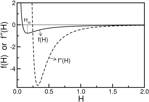
The final states of the evolution are obtained from the double-tangent construction for $f(H)$ in Fig. 1. The film segregates into phases with $H=H_{m}=D|R|^{1/3}/[(1+|R|)^{1/3}-|R|^{1/3}]$ and $H=\infty$. The latter value results in steepening high-curvature regions which never reach “equilibrium”. It is relevant to ask whether Eq. (4) has a static bump solution $H(X)$, with $H(X)\rightarrow H_{m}$ as $X\rightarrow\pm\infty$. Such a solution must satisfy the zero-current condition:

$$\frac{d^{2}H}{dX^{2}}-f^{\prime}(H)=c,$$ (6)

where the constant $c=0$ as the bump is flat when $X\rightarrow\pm\infty$, i.e., $d^{2}H/dX^{2}\rightarrow 0$. The first integral of Eq. (6) yields

$${\left(\frac{dH}{dX}\right)}^{2}=2\left[f(H)-f(H_{m})\right].$$ (7)

As $H=H_{m}$ is the sole minimum of $f(H)$ (see Fig. 1), the right-hand-side of Eq. (7) can only be zero at $H=H_{m}$. This immediately rules out a bump solution, which must satisfy $dH/dX=0$ at its peak position. The above scenario should be contrasted with the phase separation of $AB$ mixtures, where the system segregates into coexisting $A$-rich and $B$-rich domains. As we discuss shortly, this fundamental difference will have important consequences for the evolution morphology in thin films.

We numerically solve Eq. (4) in $d=3$ (i.e., on a $d=2$ substrate), starting with a small-amplitude ($\simeq 0.01$) random perturbation about the mean film thickness $H=1$. The parameters $D$ and $R$ were chosen so that the film is spinodally unstable at $H=1$. The system size is $V=(32L_{M})^{2}$. Periodic boundary conditions are applied at the lateral ends. A 32-point grid per $L_{M}$ was found to be sufficient when central differencing in space with half-node interpolation was combined with Gear’s algorithm for time-marching. This scheme is especially suitable for stiff equations.

Numerical Results and Discussion

In Fig. 2, we show MPS in a thin film evolving from the unstable homogeneous state. The parameter values are $R=-0.1$ and $D=0.2$. The snapshots on the left show the height field: regions with $H<1$ are unmarked, and regions with $H>1$ are marked black. The conservation law ensures that $\bar{H}=\int d\vec{X}H(\vec{X},T)/V$ is constant in time: $\bar{H}=H_{0}=1$ in this case. The frames on the right show the variation of the height field along a diagonal cross-section of the snapshots [$H(X,Y=X,T)$ vs. $X$]. The early time regime ($T=40$) corresponds to the growth of fluctuations about the homogeneous state. This growth is exponential and can be obtained from a linear stability analysis of Eq. (4) [20]: $H(\vec{X},T)=1+\delta H(\vec{X},T)$, where

$$\delta H(\vec{X},T)\simeq\exp\left\{t\nabla^{2}[f^{\prime\prime}(1)-\nabla^{2}]\right\}\delta H(\vec{X},0).$$ (8)

The growing fluctuations are saturated by the nonlinearity for $H\simeq H_{m}$ ($T=150$): there is no corresponding saturation for the regions with $H>1$. In the late stages ($T=250$), there is growth of domains with $H=H_{m}$ (flat phase). At the same time, the defects (or hills) become sharper and sharper. Domain growth is driven by the transport of liquid from smaller hills to larger hills due to the chemical-potential gradient. This transport can be hydrodynamic (when the black regions are connected, e.g., $T=150$) or diffusive (when the black regions are not connected, e.g., $T=250$).

Figure 2: Kinetics of morphological phase separation (MPS) in an unstable thin film in $d=3$. The initial condition for the evolution consisted of uniformly-distributed small-amplitude random fluctuations about $H(X,Y,T=0)=1$. The parameter values were $R=-0.1$ and $D=0.2$. Other simulation details are provided in the text. The dimensionless evolution times are specified above each frame. Left: Snapshots of the height field. Regions with $H>1$ (high-curvature phase) are marked in black, whereas those with $H<1$ (flat phase) are unmarked. Right: Variation of the height field along a diagonal cross-section ($Y=X$) of the snapshots.

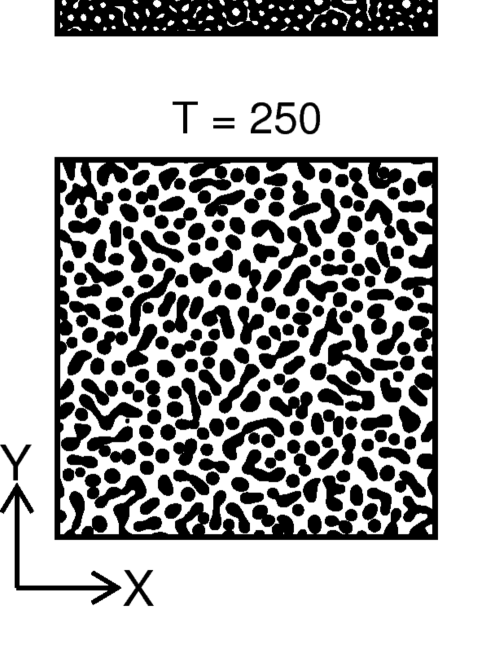
Notice that the morphology evolves continuously in Fig. 2: from bicontinuous ($T=40$) to circular domains of flat phase ($T=150$) to droplets of high-curvature phase ($T=250$). We expect that the system enters a scaling regime for $T\gtrsim 250$, where the morphology becomes self-similar and only the domain size grows. A similar evolution is seen for much thicker films with $D=0.8$ in Fig. 3. As expected, the time-scales of MPS are much longer for the thick film. The statistical results we show subsequently correspond to the film with $D=0.2$, whose evolution is shown in Fig. 2.

Figure 3: Analogous to Fig. 2, but for the parameter values $R=-0.1$ and $D=0.8$ (corresponding to a much thicker film).

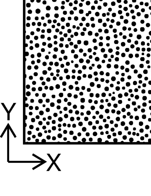
Let us present some simple arguments to understand the evolution of the scaling morphology in Fig. 2 (e.g., $T=250$) and Fig. 3 (e.g., $T=9.7\times 10^{5}$). Let $L(T)$ and $H_{d}(T)$ denote the characteristic size and height of a droplet of the high-curvature phase at time $T$. If the number of droplets in the system is $N(T)$, the amount of surplus liquid in the defects $\sim NL^{2}H_{d}$. The corresponding depletion of liquid in the flat domains is $(V-NL^{2})(1-H_{m})$, where $V$ is the substrate area. As there is a conservation of liquid, we have

$$NL^{2}H_{d}\simeq(V-NL^{2})(1-H_{m}),$$ (9)

or

$$\phi(T)\simeq\frac{(1-H_{m})}{L^{2}(H_{d}+1-H_{m})}\simeq\frac{(1-H_{m})}{L^{2}H_{d}}.$$ (10)

In Eq. (10), $\phi(T)=N(T)/V$ denotes the number of droplets per unit area. In the final step of Eq. (10), we have neglected $(1-H_{m})$ (which is constant) with respect to $H_{d}$ (which grows).

How do these droplets grow with time? Their coarsening proceeds via an evaporation-condensation mechanism. The smaller droplets evaporate and their material is diffusively transported to the larger droplets through the flat domains. The chemical potential at a point is estimated as

$$\mu=f^{\prime}(H)-\nabla^{2}H.$$ (11)

We assume that the droplets have a conical profile (cf. Fig. 2) with the height

$$H(r)\simeq H_{d}-(H_{d}-1)\left(\frac{r}{L}\right)^{n},$$ (12)

where the droplet is centered at $r=0$, and $n$ is the profile exponent. Then

$$\nabla^{2}H=\frac{1}{r}\frac{\partial}{\partial r}\left(r\frac{\partial H}{\partial r}\right)\simeq-\frac{\left(H_{d}-1\right)n^{2}}{rL}.$$ (13)

Thus, we estimate the chemical potential at the droplet boundary ($H=1$) as

$$\mu\simeq f^{\prime}(1)+\frac{(H_{d}-1)n^{2}}{L^{2}}\simeq f^{\prime}(1)+\frac{H_{d}n^{2}}{L^{2}}.$$ (14)

A better estimate of the chemical potential can be obtained by integrating over the droplet. The resultant value is the same as that in Eq. (14) up to geometric prefactors.

The chemical-potential gradient occurs over flat domains (with $H=H_{m}$) of size $\sim L$, and the corresponding current is

$$J\simeq-M(H_{m})|\vec{\nabla}\mu|\simeq\frac{H_{m}^{3}H_{d}n^{2}}{L^{3}}.$$ (15)

Thus, the droplets grow as

$$\frac{dL}{dT}\sim\frac{H_{m}^{3}H_{d}n^{2}}{L^{3}}.$$ (16)

In the scaling regime, we expect $H_{d}\sim L$ so that $L(T)\sim{(H_{m}^{3}T)}^{1/3}$. This growth law is well known in the context of phase-separation kinetics, and is referred to as the Lifshitz-Slyozov (LS) growth law [1, 21]. In earlier work [12, 13], we have demonstrated that MPS in the $d=2$ film (i.e., on a $d=1$ substrate) also obeys the LS growth law. The above arguments apply for $d=2$ films also, except when $n=1$ in Eq. (12).

There are several experimental tools to quantitatively characterize the MPS evolution morphologies. The correlation function of the height field is defined as

$$C(\vec{r},T)\equiv C(r,T)=\langle\delta H(\vec{X},T)\delta H(\vec{X}+\vec{r},T)\rangle,$$ (17)

where $\delta H$ ($=H-H_{0}$) denotes the fluctuation in the height field. The angular brackets in Eq. (17) denote an averaging over independent runs. The statistical results presented here are obtained as an average over $10$ runs. The correlation function depends only on the distance $r$ (the magnitude of $\vec{r}$) because the system is translationally invariant and isotropic. In scattering experiments with, e.g., light, X-rays, neutrons, etc., we measure the structure factor, which is the Fourier transform of $C(\vec{r},T)$ with wave-vector $\vec{k}$:

$$S(\vec{k},T)\equiv S(k,T)=\int d\vec{r}\,e^{i\vec{k}\cdot\vec{r}}C(\vec{r},T).$$ (18)

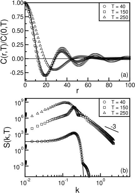
Let us present numerical results for the statistical quantities defined above. In Fig. 4(a), we plot the spherically-averaged correlation function [$C(r,T)/C(0,T)$ vs. $r$] for the evolution depicted in Fig. 2. At early times, linear theory applies and the corresponding structure factor is [20]

$$S_{\textrm{lin}}(k,T)\simeq AV\exp\left[2k^{2}\left(\alpha-k^{2}\right)T\right],$$ (19)

where $A$ is the amplitude of initial fluctuations, $\langle\delta H(\vec{X},0)\delta H(\vec{X^{\prime}},0)\rangle=A\delta(\vec{X}-\vec{X^{\prime}})$. In Eq. (19), $V$ denotes the system volume, and $\alpha=-f^{\prime\prime}(1)$. The early-time correlation function is obtained as the inverse Fourier transform of $S_{\textrm{lin}}(k,T)$:

$$C_{\textrm{lin}}(r,T) = AV\int\frac{d\vec{k}}{(2\pi)^{2}}e^{-i\vec{k}\cdot\vec{r}}\exp\left[2k^{2}\left(\alpha-k^{2}\right)T\right]$$ (20)

$$= \frac{AV}{2\pi}\int_{0}^{\infty}dk\,kJ_{0}(kr)\exp\left[2k^{2}\left(\alpha-k^{2}\right)T\right].$$

The solid line in Fig. 4(a) denotes the expression for $C_{\textrm{lin}}(r,T)/C_{\textrm{lin}}(0,T)$ from Eq. (20) with $T=40$. It is in excellent agreement with the numerical data for $T=40$. As time goes on, the fluctuations grow exponentially and linear theory ceases to hold. There is no change in the length scale during the exponential growth regime – hence, the zero-crossings of the correlation function at $T=150$ in Fig. 4(a) are comparable to those for $T=40$. (The length-scale data shown later demonstrates that domain growth occurs for $T\gtrsim 150$.) There is a crossover in $C(r,T)$, as expected from the morphological evolution seen in Fig. 2. The snapshot at $T=250$ is indicative of the scaling morphology, viz., droplets of the high-curvature phase in a background of the flat phase. In the late stages, we expect dynamical scaling of $C(r,T)$ and $S(k,T)$ [22, 1]:

$$C(r,T) = g(r/L),$$

$$S(k,T) = L^{d}f(kL),$$ (21)

where $L$ is the characteristic length scale. In Eq. (21), $g(x)$ and $f(p)$ are scaling functions which do not depend on time. In Fig. 4(a), the correlation function at $T=250$ lies in the scaling regime.

In Fig. 4(b), we plot the spherically-averaged structure factor [$S(k,T)$ vs. $k$, on a log-log scale] for the same times as in Fig. 4(a). As before, there is a crossover in the functional form of the structure factor. The data set for $T=40$ corresponds to the linear regime, and is in good agreement with the expression in Eq. (19). Notice that the linear theory is not valid at very large values of $k$ ($\gtrsim 0.5$) where we see effects of discreteness of the simulation lattice. The data set at $T=250$ corresponds to the asymptotic scaling form in Eq. (21). The peak location [$k_{m}(T)\sim L^{-1}$] moves to smaller values as the characteristic length scale grows. There is a shoulder at higher values of $k$, which reflects the second length scale apparent in the snapshots in Fig. 2. This shoulder disappears as we approach the asymptotic droplet morphology. Finally, the tail of the structure factor does not show the Porod tail [23], $S(k,T)\sim k^{-(d+1)}$ at large $k$, which is characteristic of phase-separating systems [21]. The Porod tail arises from scattering off sharp interfaces – however, the MPS morphology in Fig. 2 does not have any equilibrium interfaces at all.

Figure 4: Statistical quantities for the evolution depicted in Fig. 2. These are obtained on $(32L_{M})^{2}$ systems as an average over $10$ independent runs. (a) Plot of the spherically-averaged correlation function $C(r,T)/C(0,T)$ vs. $r$. The solid line denotes the result from linear theory in Eq. (20), evaluated at $T=40$. (b) Plot of the spherically-averaged structure factor $S(k,T)$ vs. $k$. The solid line denotes the expression in Eq. (19), evaluated at $T=40$. The line with slope $-3$ refers to Porod’s law in $d=2$, $S(k,T)\sim k^{-(d+1)}$ for large $k$. The Porod law characterizes scattering off sharp interfaces [23, 21]. In the unstable thin film, there are no equilibrium interfaces as there is only one homogeneous phase.

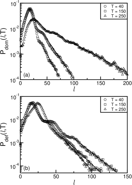
An alternative method of characterizing the growth morphology is via the probability distribution $P(l,T)$ of domain size $l$. Consider a typical snapshot in Fig. 2. We examine the variation of the height field in both the $x$- and $y$-directions, and keep track of the “zero”-crossings (where $H=1$, the average height). This yields the distribution of sizes for the flat domains, as well as the defects or hills. In Fig. 5(a), we plot the domain-size distribution $P_{\textrm{dom}}(l,T)$ vs. $l$. This quantity also shows the expected crossover from early to late times. The data set for $T=40$ has a broader distribution than the data set for $T=150$, though the peak positions are similar. The $T=40$ morphology has a broader distribution because it still contains modes with various length scales – these are dominated by the most unstable wavelength ($L_{M}$) as the fluctuations grow. The peak positions at $T=40,150$ are comparable because there is no domain growth in the early exponential regime. At later times, the domains coarsen and the peak position of $P_{\textrm{dom}}(l,T)$ shifts to the right [see data set for $T=250$ in Fig. 5(a)]. The functional form at $T=250$ corresponds to the asymptotic scaling function $p_{\textrm{dom}}(x)$, which is defined as

$$P_{\textrm{dom}}(l,T)=L^{-1}p_{\textrm{dom}}(l/L).$$ (22)

We make two further observations about $P_{\textrm{dom}}(l,T)$. First, the plots at early times ($T=40,150$) show a marked shoulder, consistent with our observation of a two-scale morphology in the snapshots of Fig. 2, and the structure factors of Fig. 4(b). This shoulder disappears as we enter the asymptotic scaling regime. Second, the tail of the distribution decays exponentially, i.e., linearly on the semi-log plot in Fig. 5(a). This is typical of morphologies with well-defined characteristic scales, and has been observed earlier in the context of phase-separation morphologies [24].

In Fig. 5(b), we plot the defect-size distribution [$P_{\textrm{def}}(l,T)$ vs. $l$] at the same times as in Fig. 5(a). This plot shows the same general features as Fig. 5(a).

Figure 5: Probability distributions of domain and defect sizes for the evolution depicted in Fig. 2. The data is plotted on a linear-log scale. The solid lines denote exponential fits to the tail region. (a) Domain-size distribution, $P_{\textrm{dom}}(l,T)$ vs. $l$. (b) Defect-size distribution, $P_{\textrm{def}}(l,T)$ vs. $l$.

Finally, in Fig. 6, we study the growth of the characteristic length scale. We use three different measures of the length scale, obtained from the statistical quantities introduced earlier:
(a) $L_{C}$, the length scale up to which $C(r,T)$ decays to half its maximum value (which arises at $r=0$).
(b) $L_{S}$, the inverse of the first moment of $S(k,T)$: $L_{S}={\langle k\rangle}^{-1}$ with

$$\langle k\rangle=\frac{\int_{0}^{\infty}{dk\,kS(k,T)}}{\int_{0}^{\infty}dk\,S(k,T)}.$$ (23)

(c) $L_{P}$, the average domain size from the relevant probability distribution:

$$L_{P}=\int_{0}^{\infty}dl\,lP_{\textrm{dom}}(l,T).$$ (24)

Figure 6: Time-dependence of the characteristic length scale for the evolution in Fig. 2. We show data for three measures of the length scale: $L_{C},L_{S}$, and $L_{P}$, obtained from $C(r,T),S(k,T)$, and $P_{\textrm{dom}}(l,T)$, respectively.

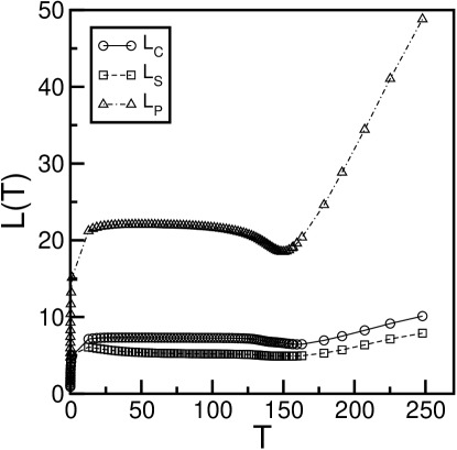
We show the time-dependence of these length scales in Fig. 6. It is interesting to note that all the different length scales show the same physical behavior. There is an early regime (up to $T\simeq 150$), where the initial fluctuations grow exponentially but there is almost no change in the length scale. In the context of phase-separation kinetics, this is referred to as the Cahn-Hilliard-Cook (CHC) regime. This is followed by an intermediate regime, where nonlinear effects saturate the growing fluctuations. The system segregates into domains of the flat phase and defects of the high-curvature phase. In the late stages ($T>175$), there is growth of domains. It is not possible to ascertain the asymptotic growth exponent from our present results, which only access a small window in the scaling regime. For this, we require 1-2 further decades of growth, which would be computationally very expensive. The numerical difficulty in accessing the late stages can be understood as follows. Recall that the interfaces become progressively steeper with time. Therefore, we need a corresponding reduction of the mesh size in space (and time) to resolve the interfaces properly.

Summary

Let us conclude this paper with a brief summary. We have undertaken a comprehensive numerical study of morphological phase separation (MPS) in unstable liquid films. In particular, we have used several experimentally relevant tools to quantitatively characterize the emergent morphologies. The statistical quantities we measure are the correlation function, structure factor, domain-size and defect-size probability distributions, and the corresponding growth laws. The study of these properties provides a complete picture of the evolution dynamics. We make several important predictions in this context. At late times, the system should enter a scaling regime, where the above quantities show dynamical scaling, i.e., the morphology becomes self-similar in time. We hope that our numerical study will motivate fresh experiments on unstable thin films.

There are important analogies and differences between MPS in thin films and phase-separation kinetics in binary mixtures. We have highlighted some of these features in this paper. A crucial difference between the two systems is the nature of the coarsening domains and defects. The unstable film segregates into droplets of a high-curvature phase (defects), separated by domains of a flat phase. On the other hand, the unstable $AB$ mixture segregates into coexisting domains of $A$-rich and $B$-rich phases, which are separated by near-equilibrium interface defects. This difference has important consequences for the evolution morphologies and their quantitative properties.

R.K. acknowledges the financial support of the Department of Science and Technology, India.

References

- [1] Kinetics of Phase Transitions, ed. S. Puri and V. K. Wadhawan, CRC Press, Boca Raton, Florida, 1st edn, 2009.
- [2] P.G. de Gennes, Rev. Mod. Phys., 1985, 57, 827.
- [3] A. Oron, S.H. Davis and S.G. Bankoff, Rev. Mod. Phys., 1997, 69, 931.
- [4] D. Bonn, J. Eggers, J. Meunier, and E. Rolley, Rev. Mod. Phys., 2009, 81, 739.
- [5] R.V. Craster and O.K. Matar, Rev. Mod. Phys., 2009, 81, 1131.
- [6] A. Sharma and R. Khanna, Phys. Rev. Lett., 1998, 81, 3463.
- [7] R. Khanna, A. Sharma, and G. Reiter, Eur. Phys. J. E, 2000, 2, 1.
- [8] S. Puri, in Ref. [1].
- [9] A. J. Bray, Adv. Phys., 1994, 43, 357.
- [10] K. Binder and P. Fratzl, Phase Transformations in Materials, ed. G. Kostorz, Wiley-VCH, Weinheim, New York, 2001.
- [11] A. Onuki, Phase Transition Dynamics, Cambridge University Press, Cambridge, UK, 2002.
- [12] R. Khanna, N. K. Agnihotri, M. Vashishtha, A. Sharma, P. K. Jaiswal and S. Puri, Phys. Rev. E, 2010, 82, 011601.
- [13] M. Vashishtha, P. K. Jaiswal, R. Khanna, S. Puri and A. Sharma, Phys. Chem. Chem. Phys., 2010, 12, 12964.
- [14] R. Khanna, N. K. Agnihotri and A. Sharma, in Ref. [1].
- [15] A. Sharma and A.T. Jameel, J. Coll. Int. Sci., 1993, 161, 190.
- [16] A.T. Jameel and A. Sharma, J. Coll. Int. Sci., 1994, 164, 416.
- [17] A. Sharma and G. Reiter, Phase Transitions, 2002, 75, 377.
- [18] E. Ruckenstein and R. K. Jain, J. Chem. Soc. Faraday Trans., 1974, 70, 132.
- [19] R. Khanna, A.T. Jameel and A. Sharma, Ind. Eng. Chem. Res., 1996, 35, 3081.
- [20] P. K. Jaiswal, M. Vashishtha, R. Khanna and S. Puri, J. Phys. Chem. B, 2011, 115, 4399.
- [21] Y. Oono and S. Puri, Phys. Rev. Lett., 1987, 58, 836; Phys. Rev. A, 1988, 38, 434; S. Puri and Y. Oono, Phys. Rev. A, 1988, 38, 1542.
- [22] K. Binder and D. Stauffer, Phys. Rev. Lett., 1974, 33, 1006.
- [23] G. Porod, Small-Angle X-Ray Scattering, ed. O. Glatter and O. Kratky, Academic Press, New York, 1982.
- [24] S. Puri, unpublished.