A simple stochastic reactive transport model

Abstract.

We introduce a discrete time microscopic single particle model for kinetic transport. The kinetics is modeled by a two-state Markov chain, the transport by deterministic advection plus a random space step. The position of the particle after $n$ time steps is given by a random sum of space steps, where the size of the sum is given by a Markov binomial distribution (MBD). We prove that by letting the length of the time steps and the intensity of the switching between states tend to zero linearly, we obtain a random variable $S(t)$, which is closely connected to a well known (deterministic) PDE reactive transport model from the civil engineering literature. Our model explains (via bimodality of the MBD) the double peaking behavior of the concentration of the free part of solutes in the PDE model. Moreover, we show for instantaneous injection of the solute that the partial densities of the free and adsorbed part of the solute at time $t$ do exist, and satisfy the partial differential equations.

Key words.Markov binomial distribution, reactive transport, kinetic adsorption, solute transport, multi-modality, double-peak.

MSC: 60J20, 60J10

1. Introduction

We consider a mathematical model for the displacement of a solute through a medium which apart from a constant flow (advection) and a dispersion (diffusion) interacts with the medium by intermittent adsorption (the kinetics). Our goal is to connect a stochastic single particle model to the well known deterministic model which describes this process by a pair of partial differential equations.

In Section 2 we give an introduction to the deterministic reactive transport model (as e.g. in [10]) characterized by a pair of partial differential equations.

In Section 3 we give our simple discrete time microscopic single particle stochastic reactive transport model. In Section 4 we calculate the probability generating functions of the Markov binomial distribution (MBD) which is described in Section 3. These are helpful to consider the convergence of our simple discrete time stochastic model by letting the time step go to zero. This will be discussed in Section 5. In Section 6 we compare our discrete time model with the obvious continuous time model.

In Section 7 we show for instantaneous injection of the solute that the partial probability densities of the free and adsorbed parts of the solute do satisfy the PDE’s defined in Section 2. In Section 8 we compute the means and variances of our stochastic reactive transport model. Actually our formula fills a gap in [10]: since the authors erroneously state that the variances are linear in the initial distribution, they only give the result for two initial distributions (this might be connected to their formula (22), which is incorrect).

In Section 9 we study the probability density function of our stochastic reactive transport model. This gives us a new and more precise point of view at the double peaking behavior in the concentration of the free part of the solute discussed by Michalak and Kitanidis in [10].

2. The PDE reactive transport model

We describe shortly the model used by Michalak and Kitanidis in [10] (see [9] for a more extensive treatment). Given is a solute that has a sorbed part that does not move, and a free part that moves in the $x$-direction by advection and dispersion. Let $C_{\textsc{F}}(t,x)$ and $C_{\textsc{A}}(t,x)$ denote the concentration functions of the free and the adsorbed part of the solute at time $t$ at position $x$. By applying mass conservation and Fick’s law one can set up the following pair of differential equations:

(1) $$\begin{split}\frac{{\partial C_{\textsc{F}}(t,x)}}{{\partial t}}+\frac{{\partial C_{\textsc{A}}(t,x)}}{{\partial t}}&=D\frac{{\partial^{2}C_{\textsc{F}}(t,x)}}{{\partial x^{2}}}-v\frac{{\partial C_{\textsc{F}}(t,x)}}{{\partial x}},\\ \frac{{\partial C_{\textsc{A}}(t,x)}}{{\partial t}}&=-\mu C_{\textsc{A}}(t,x)+\lambda C_{\textsc{F}}(t,x).\end{split}$$

Here $D$ is called the dispersion coefficient and $v$ the advection velocity. The parameters $\lambda$ and $\mu$ denote the rates of changes as described in Figure 1, with $\lambda$ for the change from free to adsorbed and $\mu$ for the change from adsorbed to free.

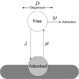
Figure 1. The schematic description of the kinetic transport model.

The initial and boundary conditions are given by

$$\begin{split}C_{\tau}(0,x)=\nu_{\tau}\delta(x),\quad\lim_{x\rightarrow\infty}C_{\tau}(t,x)=\lim_{x\rightarrow\infty}\frac{\partial C_{\tau}(t,x)}{\partial x}=0\quad\textrm{for}~{}t\geq 0,~{}\tau\in\{{\textsc{F}},{\textsc{A}}\}\end{split}$$

where $(\nu_{\textsc{F}},\nu_{\textsc{A}})$ is a probability vector and $\delta$ the Dirac delta function.

Michalak and Kitanidis have a slightly different set up, where the basic quantities are the aqueous concentration $C$ and the contaminant mass sorbed per mass of aquifer solids $S$. The connection is given by

$$C_{\textsc{F}}=\eta C,\quad C_{\textsc{A}}=\rho S,$$

where $\eta$ is the porosity and $\rho$ mass of aquifer solids per total volume.

Also, Michalak and Kitanidis do not directly use $\lambda$ and $\mu$, but rather consider a distribution coefficient $K_{d}$ and a mass transfer coefficient $k$, which are given by

$$\lambda=\frac{\rho K_{d}}{\eta}k,\quad\mu=k.$$

The main goal of the authors of [10] is to obtain closed form expressions for the $m^{th}$ normalized moments for the free and adsorbed phase, defined by

$${M}_{\tau}^{(m)}(t)=\frac{1}{M_{\tau}^{(0)}(t)}\int\limits_{-\infty}^{+\infty}{x^{m}C_{\tau}(t,x)\,\mathrm{d}x},\quad\tau\in\{{\textsc{F}},{\textsc{A}}\},$$

where the normalizing constants are given by ${M}_{\tau}^{(0)}(t)={\displaystyle\int\limits}C_{\tau}(t,x)\,\mathrm{d}x.$

These moments (for $m=1$ and $m=2$) are obtained in [10] by taking Fourier transforms in the partial differential equations (1), and differentiating. We copy here the formula from ([10], page 2136) for the normalized second central moment $\mu_{2}^{*}(t)$ where the solute is in the free phase both at time 0 and at time $t$:

(2) $$\begin{split}\mu_{2}^{*}(t)&={\frac{{t}^{2}\mathcal{A}{v}^{2}\beta\,\left(\beta-1\right)^{2}}{\left(\beta+1\right)^{2}\left(1+\beta\,\mathcal{A}\right)^{2}}}+t\left({\frac{2{\it D}}{\beta+1}}+{\frac{2{v}^{2}\beta}{k\left(\beta+1\right)^{3}}}\right)\\ &\hskip 28.45274pt+t\mathcal{A}\left({\frac{4{v}^{2}\beta\,\left(-{\beta}^{2}\mathcal{A}-{\beta}^{2}-\beta+1\right)}{k\left(1+\beta\,\mathcal{A}\right)^{2}\left(\beta+1\right)^{3}}}+{\frac{2{\it D}\,\beta\,\left(\beta-1\right)}{\left(\beta+1\right)\left(1+\beta\,\mathcal{A}\right)}}\right)\\ &\hskip 42.67912pt+{\frac{2{v}^{2}\beta\,\left(1-\mathcal{A}\right)\left(3\,{\beta}^{2}\mathcal{A}-3-\beta\,(\mathcal{A}\oplus 1)\right)}{{k}^{2}\left(1+\beta\,\mathcal{A}\right)^{2}\left(\beta+1\right)^{4}}}+{\frac{4{\it D}\,\beta\,\left(1-\mathcal{A}\right)}{k\left(1+\beta\,\mathcal{A}\right)\left(\beta+1\right)^{2}}}.\end{split}$$

Here Michalak and Kitanidis have made the following abbreviations:

$$\beta=\frac{\rho K_{d}}{\eta}=\frac{\lambda}{\mu},\quad\mathcal{A}=\mathcal{A}(t)=\exp(-(\beta+1)kt)=\exp(-(\lambda+\mu)t).$$

3. A simple stochastic reactive transport model

We describe the behavior of a single particle in the solute. Time $t$ is discretized by choosing some $n$, and dividing $[0,t]$ into $n$ intervals of the same length

$$\Delta t=t/n.$$

We suppose in such an interval of length $\Delta t$ that the particle can only be in one of the two states: ‘free ’ or ‘adsorbed ’, which we code by the letters F and A. The particle can only move when it is ‘free ’, and in this case its displacement has two components: dispersion and advection. Let $X_{k},k\geq 1$ be the displacement of the particle due to the dispersion the $k$th time that it is ‘free’. We model the $X_{k}$ as independent identically distributed random variables satisfying

(3) $${\rm E}_{\nu}\!\left[X_{k}\right]=0,\quad{\rm E}_{\nu}\!\left[X_{k}^{2}\right]=2D\Delta t\quad{\rm and}\quad{\rm E}_{\nu}\!\left[X_{k}^{3}\right]=o(\Delta t)\;\mathrm{as}\;\Delta t\downarrow 0,$$

where $D>0$, and $\nu=(\nu_{\textsc{F}},\nu_{\textsc{A}})$ is the initial distribution describing the state of the particle at time 0. When the particle is free during the interval $[(k-1)\Delta t,k\Delta t]$ for some $k$, the displacement due to advection is given by $v\Delta t$ with $v$ the (deterministic) advection velocity.

In order to model the kinetics, let $\{Y_{k},k\geq 1\}$ be a process taking values in $\{{\textsc{F}},{\textsc{A}}\}$ (we will make a choice for $\{Y_{k}\}$ below), and let

$$K_{n}=\sum_{k=1}^{n}{\bf 1}_{\{Y_{k}={\textsc{F}}\}}$$

be the occupation time of the process $\{Y_{k}\}$ in state $F$ up to time $n$.

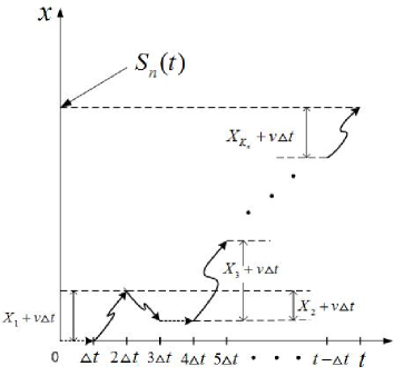
Figure 2. The position $S_{n}(t)$ of the particle at time $t=n\Delta t$ with $Y_{1}={\textsc{A}},Y_{2}={\textsc{F}},Y_{3}={\textsc{F}},Y_{4}={\textsc{A}},Y_{5}={\textsc{F}},\cdots,Y_{n}={\textsc{F}}.$

Now let $S_{n}(t)$ be the position of the particle at time $t=n\Delta t$. Then by the above (see also Figure 2) we can write $S_{n}(t)$ as

$$S_{n}(t)=\sum_{k=1}^{K_{n}}(X_{k}+v\Delta t).$$

Here we assume that $K_{n}$ is independent of the dispersion $X_{k},\,k=1,\dots,K_{n}$.

We want to compare our stochastic model with the PDE-model of Michalak and Kitanidis from Section 2. Since these authors consider the solute with given states (‘free’ or ‘adsorbed’) at time $t$, we need to consider the conditional random variables $S^{\textsc{F}}_{n}(t)$ and $S_{n}^{\textsc{A}}(t)$, i.e., the position of the particle at time $t$ given that it is ‘free’ and ‘adsorbed’ respectively at time $t=n\Delta t$. Let $K_{n}^{\tau}$ be the random variable $K_{n}$ conditioned on $Y_{n}=\tau$ with $\tau\in\{{\textsc{F}},{\textsc{A}}\}$, i.e., $K_{n}^{\tau}$ counts the number of intervals $[(k-1)\Delta t,k\Delta t],1\leq k\leq n$ where the particle is free, conditioned on the particle being in state $\tau$ in $[t-\Delta t,t]$. Then $S_{n}^{\tau}(t)$ can be written as

$$S_{n}^{\tau}(t)=\sum_{k=1}^{K_{n}^{\tau}}(X_{k}+v\Delta t).$$

The distributions of $K_{n}$ and $K_{n}^{\tau}$ are determined by the process $\{Y_{k}\}$. We take for $\{Y_{k},k\geq 1\}$ a Markov chain on the two states $\{{\textsc{F}},{\textsc{A}}\}$ with initial distribution $\nu=(\nu_{\textsc{F}},\nu_{\textsc{A}})$ and transition matrix

(4) $$P=\left[{\begin{array}[]{*{20}c}{P({\textsc{F}},{\textsc{F}})}&{P({\textsc{F}},{\textsc{A}})}\\ {P({\textsc{A}},{\textsc{F}})}&{P({\textsc{A}},{\textsc{A}})}\\ \end{array}}\right]=\left[{\begin{array}[]{*{20}c}{1-a}&{a}\\ {b}&{1-b}\\ \end{array}}\right],$$

where we assume $0<a,b<1$. The distribution of $K_{n}$ is then well known, and is called a Markov binomial distribution (MBD) (see, e.g., [5, 11]).

Clearly the stationary distribution $(\pi_{\textsc{F}},\pi_{\textsc{A}})$ of the Markov chain $\{Y_{k},k\geq 1\}$ is given by

$$\pi_{\textsc{F}}=\frac{b}{a+b},\quad\pi_{\textsc{A}}=\frac{a}{a+b}.$$

It is useful to consider the excentricities $\varepsilon_{{\textsc{F}}}$ and $\varepsilon_{{\textsc{A}}}$ of an initial distribution $\nu$ given by

$$\varepsilon_{\tau}:=\varepsilon_{\tau}(\nu)=1-\frac{\nu_{\tau}}{\pi_{\tau}},\quad\mbox{for}\quad\tau\in\{{\textsc{F}},{\textsc{A}}\}.$$

We can then write for $k\geq 1$

$${\rm P}_{\!\nu}\left(Y_{k}=\tau\right)=\pi_{\tau}(1-\varepsilon_{\tau}\,\gamma^{k-1}),$$

where $\gamma=1-a-b$ is the smallest eigenvalue of $P$ (see also [5] for the computations).

4. Probability generating functions of $K_{n}$ and $K_{n}^{\tau}$

We compute in this section the probability generating functions of $K_{n}$ and $K_{n}^{\tau}$. These are useful when we consider the convergence of the random variables $S_{n}(t)$ and $S_{n}^{\tau}(t)$ as $n$ goes to infinity.

Given $n\geq 1$, let $f_{n}$ be the probability mass function of $K_{n}$, i.e.,

$$f_{n}(j)={\rm P}_{\!\nu}\left(K_{n}=j\right).$$

In particular $f_{n}(j)=0$ if $j<0$ or $j>n$. Straightforward computations as in [16] or [5] yield that

$$f_{n+2}(j+1)=(1-b)f_{{n+1}}(j+1)+(1-a)f_{{n+1}}(j)-(1-a-b)f_{{n}}(j)$$

with initial conditions

$$\begin{split}&f_{1}(0)=\nu_{\textsc{A}},\quad f_{1}(1)=\nu_{\textsc{F}};\\ &f_{2}(0)=\nu_{\textsc{A}}(1-b),\quad f_{2}(1)=\nu_{\textsc{A}}b+\nu_{\textsc{F}}a,\quad f_{2}(2)=\nu_{\textsc{F}}(1-a).\end{split}$$

Let $G_{n}$ be the probability generating function of $K_{n}$, i.e.,

$$G_{n}(s)={\rm E}_{\nu}\!\left[s^{K_{n}}\right]=\sum_{j=0}^{n}f_{n}(j)s^{j}.$$

It follows from the above recursion equation for $f_{n}$ that

$$G_{n+2}(s)=\big{(}(1-a)s+(1-b)\big{)}G_{n+1}(s)-(1-a-b)sG_{n}(s)$$

with initial conditions

$$G_{1}(s)=\nu_{\textsc{A}}+\nu_{\textsc{F}}s,\quad G_{2}(s)=\nu_{\textsc{A}}(1-b)+(\nu_{\textsc{A}}b+\nu_{\textsc{F}}a)s+\nu_{\textsc{F}}(1-a)s^{2}.$$

By solving the difference equation of $G_{n}$ with the initial conditions we obtain the probability generating function of $K_{n}$ (see also [16]).

(5) $$\begin{split}G_{n}(s)=&~{}\frac{\nu_{\textsc{A}}\big{(}1-\beta(s)+b(s-1)\big{)}+\nu_{\textsc{F}}s\big{(}a-\beta(s)+s(1-a)\big{)}}{\alpha(s)-\beta(s)}\,\alpha(s)^{n-1}\\ &+\frac{\nu_{\textsc{A}}\big{(}1-\alpha(s)+b(s-1)\big{)}+\nu_{\textsc{F}}s\big{(}a-\alpha(s)+s(1-a)\big{)}}{\beta(s)-\alpha(s)}\,\beta(s)^{n-1},\end{split}$$

where

(6) $$\begin{split}\alpha(s)&=\frac{1}{2}\Big{(}(1-a)s+(1-b)+\sqrt{\big{(}(1-a)s-(1-b)\big{)}^{2}+4abs}\Big{)},\\ \beta(s)&=\frac{1}{2}\Big{(}(1-a)s+(1-b)-\sqrt{\big{(}(1-a)s-(1-b)\big{)}^{2}+4abs}\Big{)}.\end{split}$$

Next we are going to consider the probability generating function of $K_{n}^{\tau}$ for $\tau\in\{{\textsc{F}},{\textsc{A}}\}$. Given $n\geq 1$, let $f^{\tau}_{n}$ be the probability mass function of $K_{n}^{\tau}$, i.e.,

(7) $$f_{n}^{\tau}(j)={\rm P}_{\!\nu}\left(K_{n}^{\tau}=j\right)={\rm P}_{\!\nu}\left(K_{n}=j~{}|~{}Y_{n}=\tau\right).$$

In order to deal with $f_{n}^{\tau}$ it is simpler to deal with the partial probability mass functions

$$\hat{f}_{n}^{\tau}(j)={\rm P}_{\!\nu}\left(K_{n}=j,Y_{n}=\tau\right)=f_{n}^{\tau}(j){\rm P}_{\!\nu}\left(Y_{n}=\tau\right),$$

since these satisfy the same recursion equation as $f_{n}$:

$$\hat{f}_{n+2}^{\tau}(j+1)=(1-b)\hat{f}_{n+1}^{\tau}(j+1)+(1-a)\hat{f}_{n+1}^{\tau}(j)-(1-a-b)\hat{f}_{n}^{\tau}(j).$$

Only the initial conditions are different:

$$\begin{split}\hat{f}^{{\textsc{F}}}_{1}(0)&=0,\quad\hat{f}^{{\textsc{F}}}_{1}(1)=\nu_{\textsc{F}};\\ \hat{f}^{{\textsc{F}}}_{2}(0)&=0,\quad\hat{f}^{{\textsc{F}}}_{2}(1)=\nu_{\textsc{A}}b,\quad\hat{f}^{{\textsc{F}}}_{2}(2)=\nu_{\textsc{F}}(1-a);\end{split}$$

and

$$\begin{split}\hat{f}^{{\textsc{A}}}_{1}(0)&=\nu_{\textsc{A}},\quad\hat{f}^{{\textsc{A}}}_{1}(1)=0;\\ \hat{f}^{{\textsc{A}}}_{2}(0)&=\nu_{\textsc{A}}(1-b),\quad\hat{f}^{{\textsc{A}}}_{2}(1)=\nu_{\textsc{F}}a,\quad\hat{f}^{{\textsc{A}}}_{2}(2)=0.\end{split}$$

Then using the above recursion equation of $\hat{f}_{n}^{\tau}$ with these initial conditions, the probability generating function $G_{n}^{\tau}$ of $K_{n}^{\tau}$ can be obtained in a similar way as for $G_{n}$ (see also [16]).

(8) $$\begin{split}&G_{n}^{\textsc{F}}(s)=\sum_{j=0}^{n}f^{{\textsc{F}}}_{n}(j)s^{j}=\sum_{j=0}^{n}\frac{\hat{f}^{{\textsc{F}}}_{n}(j)}{{\rm P}_{\!\nu}\left(Y_{n}={\textsc{F}}\right)}s^{j}=\frac{1}{\pi_{\textsc{F}}(1-\varepsilon_{{\textsc{F}}}\gamma^{n-1})}\sum_{j=0}^{n}\hat{f}^{{\textsc{F}}}_{n}(j)s^{j}\\ &=\frac{\nu_{\textsc{A}}b-\nu_{\textsc{F}}\beta(s)+\nu_{\textsc{F}}(1-a)s}{(\alpha(s)-\beta(s))\pi_{\textsc{F}}(1-\varepsilon_{{\textsc{F}}}\gamma^{n-1})}\,s\alpha(s)^{n-1}+\frac{\nu_{\textsc{A}}b-\nu_{\textsc{F}}\alpha(s)+\nu_{\textsc{F}}(1-a)s}{(\beta(s)-\alpha(s))\pi_{\textsc{F}}(1-\varepsilon_{{\textsc{F}}}\gamma^{n-1})}\,s\beta(s)^{n-1},\end{split}$$

and

(9) $$\begin{split}&G_{n}^{\textsc{A}}(s)=\sum_{j=0}^{n}f^{{\textsc{A}}}_{n}(j)s^{j}=\sum_{j=0}^{n}\frac{\hat{f}^{{\textsc{A}}}_{n}(j)}{{\rm P}_{\!\nu}\left(Y_{n}={\textsc{A}}\right)}s^{j}=\frac{1}{\pi_{\textsc{A}}(1-\varepsilon_{{\textsc{A}}}\gamma^{n-1})}\sum_{j=0}^{n}\hat{f}^{{\textsc{A}}}_{n}(j)s^{j}\\ &=\frac{\nu_{\textsc{A}}(1-b)+\nu_{\textsc{F}}as-\nu_{\textsc{A}}\beta(s)}{(\alpha(s)-\beta(s))\pi_{\textsc{A}}(1-\varepsilon_{{\textsc{A}}}\gamma^{n-1})}\,\alpha(s)^{n-1}+\frac{\nu_{\textsc{A}}(1-b)+\nu_{\textsc{F}}as-\nu_{\textsc{A}}\alpha(s)}{(\beta(s)-\alpha(s))\pi_{\textsc{A}}(1-\varepsilon_{{\textsc{A}}}\gamma^{n-1})}\,\beta(s)^{n-1}.\end{split}$$

5. Towards continuous time

To get closer to the PDE model in Section 2, we have to fix $t=n\Delta t>0$ and then let the time step $\Delta t$ tend to $0$. Hence $n$ goes to infinity. We consider the rates of changes $\lambda$ and $\mu$ from Section 2. Since the probability that a particle changes its state is proportional to the length of the time step $\Delta t$ (if $\Delta t$ is small), we should put

(10) $$a=\lambda\Delta t=\frac{\lambda t}{n},\qquad b=\mu\Delta t=\frac{\mu t}{n}$$

in the transition matrix $P$ in (4). Under this assumption, we will show in this section that the random variables $S_{n}(t)$ and $S_{n}^{\tau}(t)$ defined in Section 3 converge in distribution to some random variables $S(t)$ and $S^{\tau}(t)$ respectively. To achieve this, we first consider the characteristic function $\varphi_{t,n}$ of $S_{n}(t)$, i.e.,

$$\varphi_{t,n}(u)={\rm E}_{\nu}\!\left[\mathrm{e}^{iuS_{n}(t)}\right]={\rm E}_{\nu}\!\left[\mathrm{e}^{iu\sum_{k=1}^{K_{n}}(X_{k}+v\Delta t)}\right]=G_{n}\Big{(}{\rm E}_{\nu}\!\left[\mathrm{e}^{iu(X_{1}+v\Delta t)}\right]\Big{)},$$

where $G_{n}$ is the generating function of $K_{n}$ given in (5). It is well known that (cf. [2])

$$\begin{split}&\Big{|}{\rm E}_{\nu}\!\left[\mathrm{e}^{iu(X_{1}+v\Delta t)}\right]-\sum_{k=0}^{2}\frac{(iu)^{k}}{k!}{\rm E}_{\nu}\!\left[(X_{1}+v\Delta t)^{k}\right]\Big{|}\\ \leq&\;\frac{|u|^{3}}{3!}{\rm E}_{\nu}\!\left[\big{|}X_{1}+v\Delta t\big{|}^{3}\right]=o(\Delta t)=o\big{(}\frac{1}{n}\big{)},\end{split}$$

where the last equalities hold since ${\rm E}_{\nu}\!\left[X_{1}^{3}\right]=o(\Delta t)$ in Equation (3) and $t$ is always assumed to be fixed. We then obtain by (3) that

(11) $$\begin{split}{\rm E}_{\nu}\!\left[\mathrm{e}^{iu(X_{1}+v\Delta t)}\right]&=1+iu{\rm E}_{\nu}\!\left[X_{1}+v\Delta t\right]-\frac{u^{2}}{2}{\rm E}_{\nu}\!\left[(X_{1}+v\Delta t)^{2}\right]+o\big{(}\frac{1}{n}\big{)}\\ &=1+\frac{tu(iv-Du)}{n}+o\big{(}\frac{1}{n}\big{)}=1+\frac{z}{n}+o\big{(}\frac{1}{n}\big{)},\end{split}$$

defining

$$z:=tu(iv-Du).$$

Substituting (10) and (11) into Equation (6) and letting $n$ go to infinity, we obtain

$$\begin{split}&\quad\alpha\Big{(}{\rm E}_{\nu}\!\left[\mathrm{e}^{iu(X_{1}+v\Delta t)}\right]\Big{)}^{n}=\alpha\Big{(}1+\frac{z}{n}+o\big{(}\frac{1}{n}\big{)}\Big{)}^{\!n}\\ &=\left(\frac{(1-\frac{\lambda t}{n})(1+\frac{z}{n})+(1-\frac{\mu t}{n})+\sqrt{\big{(}(1-\frac{\lambda t}{n})(1+\frac{z}{n})-(1-\frac{\mu t}{n})\big{)}^{2}+\frac{4\lambda\mu t^{2}}{n^{2}}(1+\frac{z}{n})}}{2}+o\big{(}\frac{1}{n}\big{)}\right)^{n}\\ &\longrightarrow\;\exp{\Big{(}\frac{1}{2}\Big{[}z-(\lambda+\mu)t+\sqrt{\big{(}z+t(\mu-\lambda)\big{)}^{2}+4\lambda\mu t^{2}}\Big{]}\Big{)}}\\ &\quad=\exp{\Big{(}-\frac{t}{2}\Big{[}Du^{2}-ivu+\lambda+\mu-\sqrt{(Du^{2}-ivu+\lambda-\mu)^{2}+4\lambda\mu}\,\Big{]}\Big{)}}.\end{split}$$

Here we chose the complex square root of $(Du^{2}-ivu+\lambda-\mu)^{2}+4\lambda\mu$ with positive real part.

Similarly, the corresponding limit for $\beta\big{(}{\rm E}_{\nu}\!\left[\mathrm{e}^{iu(X_{1}+v\Delta t)}\right]\big{)}^{n}$ is obtained by replacing the minus in front of the square root of the last equality by a plus. It seems convenient to introduce the following two notations:

(12) $$\begin{split}\theta_{\textsc{A}}=\theta_{\textsc{A}}(u):=&\sqrt{(Du^{2}-ivu+\lambda-\mu)^{2}+4\lambda\mu}-(Du^{2}-ivu),\\ \theta_{\textsc{F}}=\theta_{\textsc{F}}(u):=&\sqrt{(Du^{2}-ivu+\lambda-\mu)^{2}+4\lambda\mu}+(Du^{2}-ivu).\end{split}$$

Then the limits for $\alpha\big{(}{\rm E}_{\nu}\!\left[\mathrm{e}^{iu(X_{1}+v\Delta t)}\right]\big{)}^{n}$ and $\beta\big{(}{\rm E}_{\nu}\!\left[\mathrm{e}^{iu(X_{1}+v\Delta t)}\right]\big{)}^{n}$ can be rewritten as:

$$\begin{split}\lim\limits_{n\rightarrow\infty}\alpha\big{(}{\rm E}_{\nu}\!\left[\mathrm{e}^{iu(X_{1}+v\Delta t)}\right]\big{)}^{n}&=\exp{\big{(}(\theta_{\textsc{A}}-\lambda-\mu)t/2\big{)}},\\ \lim\limits_{n\rightarrow\infty}\beta\big{(}{\rm E}_{\nu}\!\left[\mathrm{e}^{iu(X_{1}+v\Delta t)}\right]\big{)}^{n}&=\exp{\big{(}-(\theta_{\textsc{F}}+\lambda+\mu)t/2\big{)}}.\end{split}$$

So we obtain by substituting (10) and (11) into Equation (5) that the limit of the characteristic functions $\varphi_{t,n}$ of $S_{n}(t)$ is a function $\varphi_{t}$ given by

(13) $$\varphi_{t}(u)=\mathrm{e}^{(\theta_{\textsc{A}}-\lambda-\mu)t/2}\frac{\nu_{\textsc{A}}\theta_{\textsc{F}}+\nu_{\textsc{F}}\,\theta_{\textsc{A}}+\lambda+\mu}{\theta_{\textsc{A}}+\theta_{\textsc{F}}}+\mathrm{e}^{-(\theta_{\textsc{F}}+\lambda+\mu)t/2}\frac{\nu_{\textsc{A}}\theta_{\textsc{A}}+\nu_{\textsc{F}}\,\theta_{\textsc{F}}-\lambda-\mu}{\theta_{\textsc{A}}+\theta_{\textsc{F}}}.$$

It is easy to see that $\varphi_{t}$ is continuous at $u=0$. This implies that there exists a random variable, which we call $S(t)$, such that as $n\rightarrow\infty$

$$S_{n}(t)\longrightarrow S(t)\quad\textrm{in~{}~{}distribution.}$$

Next we are going to consider the convergence of the random variable $S^{{\textsc{F}}}_{n}(t)$ as $n$ goes to infinity. In a similar way as for $S_{n}(t)$ we consider the characteristic function $\varphi^{{\textsc{F}}}_{t,n}$ of $S^{{\textsc{F}}}_{n}(t)$, i.e.,

$$\varphi^{{\textsc{F}}}_{t,n}(u)={\rm E}_{\nu}\!\left[\mathrm{e}^{iuS^{{\textsc{F}}}_{n}(t)}\right]=G^{{\textsc{F}}}_{n}\Big{(}{\rm E}_{\nu}\!\left[\mathrm{e}^{iu(X_{1}+v\Delta t)}\right]\Big{)},$$

where $G^{{\textsc{F}}}_{n}$ is the probability generating function of $K_{n}^{\textsc{F}}$ given in Equation (8). Substituting (10) and (11) into Equation (8) and letting $n$ go to infinity, we obtain that the limit of the characteristic function $\varphi^{{\textsc{F}}}_{t,n}$ of $S^{{\textsc{F}}}_{n}(t)$ is a function $\varphi^{{\textsc{F}}}_{t}$ given by

(14) $$\varphi^{{\textsc{F}}}_{t}(u)=\mathrm{e}^{(\theta_{\textsc{A}}-\lambda-\mu)t/2}\frac{\nu_{\textsc{F}}(\theta_{\textsc{A}}-\lambda-\mu)+2\mu}{(\theta_{\textsc{A}}+\theta_{\textsc{F}})\pi_{\textsc{F}}(1-\varepsilon_{{\textsc{F}}}\mathcal{A})}+\mathrm{e}^{-(\theta_{\textsc{F}}+\lambda+\mu)t/2}\frac{\nu_{\textsc{F}}(\theta_{\textsc{F}}+\lambda+\mu)-2\mu}{(\theta_{\textsc{A}}+\theta_{\textsc{F}})\pi_{\textsc{F}}(1-\varepsilon_{{\textsc{F}}}\mathcal{A})},$$

where $\mathcal{A}=\mathcal{A}(t)=\exp{(-(\lambda+\mu)t)}$. Here we point out that the stationary distribution $(\pi_{\textsc{F}},\pi_{\textsc{A}})$ and the excentricities $\varepsilon_{{\textsc{F}}},\varepsilon_{{\textsc{A}}}$ do not depend on the time step $\Delta t$, since by (10)

$$\pi_{\textsc{F}}=\frac{b}{a+b}=\frac{\mu}{\lambda+\mu},~{}\pi_{\textsc{A}}=\frac{a}{a+b}=\frac{\lambda}{\lambda+\mu},~{}\varepsilon_{{\textsc{F}}}=1-\frac{\lambda+\mu}{\mu}\nu_{\textsc{F}},~{}\varepsilon_{{\textsc{A}}}=1-\frac{\lambda+\mu}{\lambda}\nu_{\textsc{A}}.$$

Again there exists a random variable, which we call $S^{{\textsc{F}}}(t)$, such that as $n\rightarrow\infty$

$$S^{{\textsc{F}}}_{n}(t)\longrightarrow S^{{\textsc{F}}}(t)\quad\textrm{in~{}~{}distribution.}$$

Similarly, substituting (10) and (11) into Equation (9) and letting $n$ go to infinity, one can show that there exists a random variable $S^{{\textsc{A}}}(t)$ such that $S^{{\textsc{A}}}_{n}(t)\longrightarrow S^{{\textsc{A}}}(t)$ in distribution as $n\rightarrow\infty$, where $S^{{\textsc{A}}}(t)$ has characteristic function:

(15) $$\varphi^{{\textsc{A}}}_{t}(u)=\mathrm{e}^{(\theta_{\textsc{A}}-\lambda-\mu)t/2}\frac{\nu_{\textsc{A}}(\theta_{\textsc{F}}-\lambda-\mu)+2\lambda}{(\theta_{\textsc{A}}+\theta_{\textsc{F}})\pi_{\textsc{A}}(1-\varepsilon_{{\textsc{A}}}\mathcal{A})}+\mathrm{e}^{-(\theta_{\textsc{F}}+\lambda+\mu)t/2}\frac{\nu_{\textsc{A}}(\theta_{\textsc{A}}+\lambda+\mu)-2\lambda}{(\theta_{\textsc{A}}+\theta_{\textsc{F}})\pi_{\textsc{A}}(1-\varepsilon_{{\textsc{A}}}\mathcal{A})}.$$

6. Modeling the kinetics with a continuous time Markov chain

In our model we used a simple discrete time set up. This will be useful in Section 9, but it is worthwhile to compare our results with a model that involves a continuous time Markov chain. Let $Y(t),t\geq 0$ denote the state of the particle at time $t$. Recall from Section 2 that $\lambda$ and $\mu$ are the rates of changes from ‘free’ to ‘adsorbed’ and ‘adsorbed’ to ‘free’ respectively. Hence it is natural to model the kinetics by a two-state continuous time Markov chain $\{Y(t),t\geq 0\}$ with initial distribution ${\rm P}_{\!\nu}\left(Y(0)=\tau\right)=\nu_{\tau},\tau\in\{{\textsc{F}},{\textsc{A}}\}$ and generator matrix

$$Q=\left(\begin{array}[]{cc}Q({\textsc{F}},{\textsc{F}})&Q({\textsc{F}},{\textsc{A}})\\ Q({\textsc{A}},{\textsc{F}})&Q({\textsc{A}},{\textsc{A}})\end{array}\right)=\left(\begin{array}[]{cc}-\lambda&\lambda\\ \mu&-\mu\end{array}\right).$$

The solute can only move when it is free, and in this case we model the displacement due to dispersion and advection as a Brownian motion with drift $v$.

A trick to deal with continuous time Markov chains is uniformization. This idea gives us an alternative way to model the $S(t)$ and $S^{\tau}(t),\tau\in\{{\textsc{F}},{\textsc{A}}\}$ obtained in Section 5. Let $\Lambda\geq\max{(\lambda,\mu)}$ be the rate of the uniformization. It follows that (see e.g. [13], page 402) the continuous time Markov chain $\{Y(t),t\geq 0\}$ can be viewed as a discrete time Markov chain $\{Z_{k},k\geq 0\}$ over the same state space $\{{\textsc{F}},{\textsc{A}}\}$ and the same initial distribution ${\rm P}_{\!\nu}\left(Z_{0}=\tau\right)=\nu_{\tau},\tau\in\{{\textsc{F}},{\textsc{A}}\}$, but with the transition matrix

$$P_{\Lambda}=\left(\begin{array}[]{cc}P({\textsc{F}},{\textsc{F}})&P({\textsc{F}},{\textsc{A}})\\ P({\textsc{A}},{\textsc{F}})&P({\textsc{A}},{\textsc{A}})\end{array}\right)=\left(\begin{array}[]{cc}1-\lambda/\Lambda&\lambda/\Lambda\\ \mu/\Lambda&1-\mu/\Lambda\end{array}\right).$$

Let $N(t)$ be the number of the state transitions up to time $t$, which is a Poisson process with rate $\Lambda$. Let $K_{N(t)}$ be the occupation time of the chain $\{Z_{k}\}$ in state F up to time $N(t)$, which is a Markov binomial distributed random variable, when conditioned on $N(t)$. Since the solute can only move when it is free and the displacement in the free state is due to dispersion and advection, we model $\mathcal{X}_{k}$, the displacement during the $k$th free interval, as a Brownian motion with drift $v$ stopped at time $T$ which is exponentially $\Lambda$ distributed. So we put

$$\mathcal{X}_{k}\stackrel{{\scriptstyle d}}{{=}}\mathcal{N}(vT,{2D}T)\quad\textrm{with}\quad T\stackrel{{\scriptstyle d}}{{=}}Exp(\Lambda).$$

Then we can write $\mathcal{H}_{\Lambda}(t)$, the position of the particle at time $t$ with respect to the uniformization at rate $\Lambda$, as:

$$\mathcal{H}_{\Lambda}(t)=\sum_{k=1}^{K_{N(t)}}\mathcal{X}_{k}.$$

Similarly, for $\tau\in\{{\textsc{F}},{\textsc{A}}\}$ we can define $\mathcal{H}_{\Lambda}^{\tau}(t)$ merely by changing $K_{N(t)}$ to the conditional random variable $K_{N(t)}^{\tau}=K_{N(t)}~{}|~{}{\{Z_{N(t)}=\tau\}}$, i.e., $\mathcal{H}_{\Lambda}^{\tau}(t)$ denotes the position of the particle at time $t$ conditioned on being in state $\tau$ at time $N(t)$.

Letting $\Lambda$ go to infinity, one can show by using the characteristic functions of $\mathcal{H}_{\Lambda}(t)$ and $\mathcal{H}_{\Lambda}^{\tau}(t)$ as in Section 5 that

$$\mathcal{H}_{\Lambda}(t)\longrightarrow S(t),\quad\mathcal{H}_{\Lambda}^{\tau}(t)\longrightarrow S^{\tau}(t)\quad\textrm{in~{}distribution},$$

where $S(t),S^{\tau}(t)$ are the same random variables as in Section 5.

It is even more natural to look at the continuous time Markov chain $\{Y(t),t\geq 0\}$ directly. Let $U(t)$ be the occupation time of the chain $\{Y(t)\}$ in state F up to time $t$, and let $f_{U(t)}$ be its probability density function. We model the displacement of the solute in the free phase as a Brownian motion with drift $v$. Then the position $H(t)$ of the particle at time $t$ can be written as a normal distribution with mean $v\,U(t)$ and variance $2D\,U(t)$. Conditional on $U(t)$ it follows from Equation (5) of [12] and Equation (13) that for $\phi>0$

$$\begin{split}\int_{0}^{\infty}{\rm E}_{\nu}\!\left[\mathrm{e}^{iuH(t)}\right]\mathrm{e}^{-\phi t}\mathrm{d}t=&~{}\int_{0}^{\infty}\int_{0}^{\infty}\mathrm{e}^{-(Du^{2}-ivu)x}\mathrm{e}^{-\phi t}f_{U(t)}(x)\,\mathrm{d}x\,\mathrm{d}t\\ =&~{}(\nu_{\textsc{F}},\nu_{\textsc{A}})\left(\begin{array}[]{cc}\lambda+\phi+Du^{2}-ivu&-\lambda\\ -\mu&\mu+\phi\end{array}\right)^{-1}{1\choose 1}\\ =&~{}\frac{\phi+\lambda+\mu+\nu_{\textsc{A}}(Du^{2}-ivu)}{(\phi+\lambda+Du^{2}-ivu)(\phi+\mu)-\lambda\mu}=\int_{0}^{\infty}{\rm E}_{\nu}\!\left[\mathrm{e}^{iuS(t)}\right]e^{-\phi t}\mathrm{d}t.\end{split}$$

Since ${\rm E}_{\nu}\!\left[\mathrm{e}^{iuS(t)}\right]$ is a continuous function of $t$ by Equation (13), it follows from Lerch’s theorem (cf. [14], page 24) that ${\rm E}_{\nu}\!\left[\mathrm{e}^{iuH(t)}\right]={\rm E}_{\nu}\!\left[\mathrm{e}^{iuS(t)}\right]$ for all $t\geq 0$. Hence $H(t)$ and $S(t)$ have the same distribution.

Similarly, for $\tau\in\{{\textsc{F}},{\textsc{A}}\}$ let $H^{\tau}(t)=H(t)~{}|~{}{\{Y(t)=\tau\}}$ be the conditional random variable denoting the position of the particle at time $t$ conditioned on being in state $\tau$ at time $t$. From the proof of Theorem 1 in [3] one obtains that for $\phi>0$

$$\begin{split}\int_{0}^{\infty}{\rm P}_{\!\nu}\left(Y(t)={\textsc{F}}\right)&{\rm E}_{\nu}\!\left[\mathrm{e}^{iuH^{\textsc{F}}(t)}\right]\mathrm{e}^{-\phi t}\mathrm{d}t=\int_{0}^{\infty}{\rm E}_{\nu}\!\left[\mathrm{e}^{iuH(t)}\textbf{1}_{\{Y(t)={\textsc{F}}\}}\right]\mathrm{e}^{-\phi t}\mathrm{d}t\\ =&~{}(\nu_{\textsc{F}},\nu_{\textsc{A}})\left(\begin{array}[]{cc}\lambda+\phi+Du^{2}-ivu&-\lambda\\ -\mu&\mu+\phi\end{array}\right)^{-1}{1\choose 0}\\ =&~{}\frac{\mu+\nu_{\textsc{F}}\phi}{(\phi+\lambda+Du^{2}-ivu)(\phi+\mu)-\lambda\mu}\\ =&~{}\int_{0}^{\infty}{\rm P}_{\!\nu}\left(Y(t)={\textsc{F}}\right){\rm E}_{\nu}\!\left[\mathrm{e}^{iu{S}^{\textsc{F}}(t)}\right]\mathrm{e}^{-\phi t}\mathrm{d}t,\end{split}$$

where the last equality follows using Equation (14) and since the limiting probability of a particle being in state $\tau$ at time $t$ is given by

(16) $${\rm P}_{\!\nu}\left(Y(t)=\tau\right)=\lim_{n\rightarrow\infty}{\rm P}_{\!\nu}\left(Y_{n}=\tau\right)=\lim_{n\rightarrow\infty}\pi_{\tau}(1-\varepsilon_{\tau}\gamma^{n-1})=\pi_{\tau}(1-\varepsilon_{\tau}\mathcal{A}(t))$$

with $\mathcal{A}(t)=\exp{(-(\lambda+\mu)t)}$. Similarly one can also show that for $\phi>0$

$$\begin{split}\int_{0}^{\infty}{\rm P}_{\!\nu}\left(Y(t)={\textsc{A}}\right){\rm E}_{\nu}\!\left[\mathrm{e}^{iuH^{\textsc{A}}(t)}\right]\mathrm{e}^{-\phi t}\mathrm{d}t&=\frac{\lambda+\nu_{\textsc{A}}(\phi+Du^{2}-ivu)}{(\phi+\lambda+Du^{2}-ivu)(\phi+\mu)-\lambda\mu}\\ &=\int_{0}^{\infty}{\rm P}_{\!\nu}\left(Y(t)={\textsc{A}}\right){\rm E}_{\nu}\!\left[\mathrm{e}^{iu{S}^{\textsc{A}}(t)}\right]\mathrm{e}^{-\phi t}\mathrm{d}t.\end{split}$$

Again, using Lerch’s theorem, it follows that $H^{\tau}(t)$ and ${S}^{\tau}(t)$ have the same distribution. Therefore our discrete time model converges in distribution to the same random variables as obtained by the natural continuous time Markov chain.

7. Densities and partial differential equations

We will show in this section that for instantaneous injection of the solute, i.e., with initial distribution $\nu=(1,0)$, the partial probability density functions $\hat{f}^{{\textsc{F}}}_{S}(t,x)$ and $\hat{f}^{{\textsc{A}}}_{S}(t,x)$ of $S^{{\textsc{F}}}(t)$ and $S^{{\textsc{A}}}(t)$ do satisfy the partial differential equations in (1).

Let $f_{S}(t,x)$ and $f_{S}^{\tau}(t,x)$ denote respectively the probability density functions of $S(t)$ and $S^{\tau}(t)$ for $\tau\in\{{\textsc{F}},{\textsc{A}}\}$. Recall from (16) that the probability of a particle being in state $\tau$ at time $t$ is given by ${\rm P}_{\!\nu}\left(Y(t)=\tau\right)=\pi_{\tau}(1-\varepsilon_{\tau}\mathcal{A}(t))$. We define the partial probability density functions of $S^{\tau}(t)$ as

(17) $$\hat{f}_{S}^{\tau}(t,x)={\rm P}_{\!\nu}\left(Y(t)=\tau\right)f^{\tau}_{S}(t,x)=\pi_{\tau}(1-\varepsilon_{\tau}\mathcal{A}(t))f_{S}^{\tau}(t,x).$$

Obviously $f_{S}(t,x)=\hat{f}^{{\textsc{F}}}_{S}(t,x)+\hat{f}^{{\textsc{A}}}_{S}(t,x)$.

Lemma 7.1.

Let $\theta_{\textsc{A}}=\theta_{\textsc{A}}(u),~{}\theta_{\textsc{F}}=\theta_{\textsc{F}}(u)$ be defined as in (12). Then

$$\lim\limits_{u\rightarrow\infty}\big{|}u^{2}\big{(}\theta_{\textsc{A}}(u)-(\lambda-\mu)\big{)}\big{|}=2\lambda\mu/D,\quad\lim\limits_{u\rightarrow\infty}|\theta_{\textsc{F}}(u)/u^{2}|=2D.$$

Proof.

It is straightforward to check these formulas. ∎

Lemma 7.2.

The probability density function $f^{{\textsc{F}}}_{S}(t,\cdot)$ of $S^{{\textsc{F}}}(t)$ can be written as

$$f^{{\textsc{F}}}_{S}(t,x)=\frac{1}{2\pi}\int\mathrm{e}^{-iux}\varphi^{{\textsc{F}}}_{t}(u)\,\mathrm{d}u,$$

where $\varphi^{{\textsc{F}}}_{t}$ is the characteristic function of $S^{{\textsc{F}}}(t)$ given in (14).

Proof.

We only need to show that $\varphi^{{\textsc{F}}}_{t}$ is integrable. Obviously $\varphi^{{\textsc{F}}}_{t}$ is a continuous function. So it suffices to show that $\int_{|u|>M}|\varphi^{{\textsc{F}}}_{t}(u)|\,\mathrm{d}u<\infty$ for some $M>0$. From Lemma 7.1 and (14) it follows that for all $|u|$ large

$$\begin{split}|\varphi^{{\textsc{F}}}_{t}(u)|&\leq\Big{|}\mathrm{e}^{(\theta_{\textsc{A}}-\lambda-\mu)t/2}\frac{\nu_{\textsc{F}}(\theta_{\textsc{A}}-\lambda-\mu)+2\mu}{(\theta_{\textsc{A}}+\theta_{\textsc{F}})\pi_{\textsc{F}}(1-\varepsilon_{{\textsc{F}}}\mathcal{A})}\Big{|}+\Big{|}\mathrm{e}^{-(\theta_{\textsc{F}}+\lambda+\mu)t/2}\frac{\nu_{\textsc{F}}(\theta_{\textsc{F}}+\lambda+\mu)-2\mu}{(\theta_{\textsc{A}}+\theta_{\textsc{F}})\pi_{\textsc{F}}(1-\varepsilon_{{\textsc{F}}}\mathcal{A})}\Big{|}\\ &\leq\frac{C_{1}}{u^{2}}+C_{2}\mathrm{e}^{-Dtu^{2}/2},\end{split}$$

where $C_{1},C_{2}$ are constants independent of $u$. This finishes the proof of the lemma. ∎

Surprisingly, Lemma 7.2 does not hold for $S^{{\textsc{A}}}(t)$, but we still have the following.

Lemma 7.3.

The distribution $\mu_{\textsc{A}}$ of the random variable $S^{\textsc{A}}(t)$ can be written as

$$\mu_{\textsc{A}}=\kappa\,\delta_{0}+(1-\kappa)\tilde{\mu}_{\textsc{A}}$$

where $\kappa=\nu_{\textsc{A}}\mathrm{e}^{-\mu t}/(\pi_{\textsc{A}}(1-\varepsilon_{{\textsc{A}}}\mathcal{A}))$ and $\tilde{\mu}_{\textsc{A}}$ is the distribution of a continuous random variable having probability density function

$$f^{{\textsc{A}}}_{S}(t,x)=\frac{1}{2\pi(1-\kappa)}\int\mathrm{e}^{-iux}\big{(}\varphi^{{\textsc{A}}}_{t}(u)-\kappa\big{)}\mathrm{d}u,$$

with $\varphi^{{\textsc{A}}}_{t}$ the characteristic function of $S^{{\textsc{A}}}(t)$ defined in (15).

Proof.

It follows from Lemma 7.1 and Equation (15) that for all $|u|$ large

(18) $$\begin{split}\Big{|}\varphi^{{\textsc{A}}}_{t}(u)-\kappa\Big{|}\leq&~{}\Big{|}\mathrm{e}^{(\theta_{\textsc{A}}-\lambda-\mu)t/2}\frac{\nu_{\textsc{A}}(\theta_{\textsc{F}}-\lambda-\mu)+2\lambda}{(\theta_{\textsc{A}}+\theta_{\textsc{F}})\pi_{\textsc{A}}(1-\varepsilon_{{\textsc{A}}}\mathcal{A})}-\frac{\nu_{\textsc{A}}\mathrm{e}^{-\mu t}}{\pi_{\textsc{A}}(1-\varepsilon_{{\textsc{A}}}\mathcal{A})}\Big{|}\\ &\quad+\Big{|}\mathrm{e}^{-(\theta_{\textsc{F}}+\lambda+\mu)t/2}\frac{\nu_{\textsc{A}}(\theta_{\textsc{A}}+\lambda+\mu)-2\lambda}{(\theta_{\textsc{A}}+\theta_{\textsc{F}})\pi_{\textsc{A}}(1-\varepsilon_{{\textsc{A}}}\mathcal{A})}\Big{|}\\ \leq&~{}\Big{|}\mathrm{e}^{(\theta_{\textsc{A}}-\lambda-\mu)t/2}\frac{2\lambda-\nu_{\textsc{A}}(\theta_{\textsc{A}}+\lambda+\mu)}{(\theta_{\textsc{A}}+\theta_{\textsc{F}})\pi_{\textsc{A}}(1-\varepsilon_{{\textsc{A}}}\mathcal{A})}\Big{|}\\ &\quad+\Big{|}\frac{\nu_{\textsc{A}}\mathrm{e}^{-\mu t}}{\pi_{\textsc{A}}(1-\varepsilon_{{\textsc{A}}}\mathcal{A})}\big{(}\mathrm{e}^{(\theta_{\textsc{A}}-\lambda+\mu)t/2}-1\big{)}\Big{|}+C_{2}\mathrm{e}^{-Dtu^{2}/2}\\ \leq&~{}C_{1}\frac{1}{u^{2}}+C_{2}\mathrm{e}^{-Dtu^{2}/2},\end{split}$$

where $C_{1},C_{2}$ are constants independent of $u$. This implies that the integrand in the lemma is integrable.

Without loss of generality we may suppose $\nu_{\textsc{A}}>0$. Using (18) we obtain that as $T\rightarrow\infty$

$$\Big{|}\frac{1}{2T}\int_{-T}^{T}\varphi^{{\textsc{A}}}_{t}(u)\mathrm{d}u-\kappa\Big{|}=\frac{1}{2T}\Big{|}\int_{-T}^{T}\Big{(}\varphi^{{\textsc{A}}}_{t}(u)-\kappa\Big{)}\mathrm{d}u\Big{|}\rightarrow\,0.$$

This implies that the point $0$ is an atom of $\mu_{\textsc{A}}$, since (cf. [2], page 306)

$$\begin{split}\mu_{\textsc{A}}(\{0\})=\lim_{T\rightarrow\infty}\frac{1}{2T}\int_{-T}^{T}\varphi^{{\textsc{A}}}_{t}(u)\mathrm{d}u=\kappa.\end{split}$$

Moreover, $0$ is the unique atom of $\mu_{\textsc{A}}$ since (cf. [2], page 306)

$$\sum_{q}(\mu_{\textsc{A}}(\{q\}))^{2}=\lim_{T\rightarrow\infty}\frac{1}{2T}\int_{-T}^{T}|\varphi^{{\textsc{A}}}_{t}(u)|^{2}\mathrm{d}u=(\mu_{\textsc{A}}(\{0\}))^{2},$$

where the sum is taken over the set of points of positive $\mu_{\textsc{A}}$ measure, and the second equality can be seen by using (18) and the fact that $\varphi^{{\textsc{A}}}_{t}(u)$ is uniformly bounded. This establishes the lemma. ∎

It follows from Lemma 7.3 that $S^{{\textsc{A}}}(t)$ is a continuous random variable if and only if $\nu=(1,0)$, i.e, for instantaneous injection of the solute. It is interesting that in this case we have the following.

Theorem 7.1.

The partial probability density functions $\hat{f}_{S}^{\tau}$ of $S^{\tau}(t)$ for $\tau\in\{{\textsc{F}},{\textsc{A}}\}$ satisfy the partial differential equations (1):

$$\begin{split}\frac{{\partial\hat{f}^{{\textsc{F}}}_{S}(t,x)}}{{\partial t}}+\frac{{\partial\hat{f}^{{\textsc{A}}}_{S}(t,x)}}{{\partial t}}&=D\frac{{\partial^{2}\hat{f}^{{\textsc{F}}}_{S}(t,x)}}{{\partial x^{2}}}-v\frac{{\partial\hat{f}^{{\textsc{F}}}_{S}(t,x)}}{{\partial x}},\\ \frac{{\partial\hat{f}^{{\textsc{A}}}_{S}(t,x)}}{{\partial t}}&=-\mu\hat{f}^{{\textsc{A}}}_{S}(t,x)+\lambda\hat{f}^{{\textsc{F}}}_{S}(t,x)\end{split}$$

for $t>0$, with initial and boundary conditions

$$\begin{split}&\hat{f}^{{\textsc{F}}}_{S}(0,x):=\delta(x),\quad\hat{f}^{{\textsc{A}}}_{S}(0,x):=0;\\ &\lim_{x\rightarrow\infty}\hat{f}_{S}^{\tau}(t,x)=\lim_{x\rightarrow\infty}\frac{\partial\hat{f}_{S}^{\tau}(t,x)}{\partial x}=0\quad\textrm{for}~{}t\geq 0,~{}\tau\in\{{\textsc{F}},{\textsc{A}}\}.\end{split}$$

Proof.

The initial conditions imply $\nu=(1,0)$. It follows from Lemma 7.2, 7.3 and Equation (17) that

$$\hat{f}^{\tau}_{S}(t,x)=\frac{1}{2\pi}\int\mathrm{e}^{-iux}\hat{\varphi}_{t}^{\tau}(u)\,\mathrm{d}u\quad\textrm{for}\quad\tau\in\{{\textsc{F}},{\textsc{A}}\},$$

where

(19) $$\hat{\varphi}_{t}^{\tau}(u)=\pi_{\tau}(1-\varepsilon_{\tau}\mathcal{A}(t))\varphi_{t}^{\tau}(u),$$

with $\varphi^{\tau}_{t}$ the characteristic functions of $S^{\tau}(t)$ given in (14) and (15) respectively. It is easy to see that $\hat{f}^{{\textsc{F}}}_{S}$ and $\hat{f}^{{\textsc{A}}}_{S}$ satisfy the initial and boundary conditions.

Using Lemma 7.1 it is not hard to check that the four functions in $u$

$$\Big{|}\frac{\partial\mathrm{e}^{-iux}\hat{\varphi}^{{\textsc{F}}}_{t}(u)}{\partial t}\Big{|},\quad\Big{|}\frac{\partial\mathrm{e}^{-iux}\hat{\varphi}^{{\textsc{A}}}_{t}(u)}{\partial t}\Big{|},\quad\Big{|}\frac{\partial\mathrm{e}^{-iux}\hat{\varphi}^{{\textsc{F}}}_{t}(u)}{\partial x}\Big{|},\quad\Big{|}\frac{\partial^{2}\mathrm{e}^{-iux}\hat{\varphi}^{{\textsc{F}}}_{t}(u)}{\partial x^{2}}\Big{|},$$

are all bounded by a function of the form $C_{1}/u^{2}+C_{2}\mathrm{e}^{-\frac{t}{2}Du^{2}}$ for $|u|$ large, where $C_{1},C_{2}$ are constants independent of $u$. Thus we can exchange the integral and differential operators in the partial differential equations (cf. [6], page 417). Hence we only need to show that

$$\begin{split}\frac{{\partial\hat{\varphi}^{{\textsc{F}}}_{t}(u)}}{{\partial t}}&=-Du^{2}\hat{\varphi}^{{\textsc{F}}}_{t}(u)+ivu\hat{\varphi}^{{\textsc{F}}}_{t}(u)-\lambda\hat{\varphi}^{{\textsc{F}}}_{t}(u)+\mu\hat{\varphi}^{{\textsc{A}}}_{t}(u),\\ \frac{{\partial\hat{\varphi}^{{\textsc{A}}}_{t}(u)}}{{\partial t}}&=-\mu\hat{\varphi}^{{\textsc{A}}}_{t}(u)+\lambda\hat{\varphi}^{{\textsc{F}}}_{t}(u).\end{split}$$

It follows from (14), (15), (19) and $\nu_{\textsc{A}}=0$ that

$$\begin{split}&-Du^{2}\hat{\varphi}^{{\textsc{F}}}_{t}(u)+ivu\hat{\varphi}^{{\textsc{F}}}_{t}(u)-\lambda\hat{\varphi}^{{\textsc{F}}}_{t}(u)+\mu\hat{\varphi}^{{\textsc{A}}}_{t}(u)\\ =&~{}(\frac{\theta_{\textsc{A}}-\theta_{\textsc{F}}}{2}-\lambda)\Big{(}\mathrm{e}^{(\theta_{\textsc{A}}-\lambda-\mu)t/2}\frac{\theta_{\textsc{A}}-\lambda+\mu}{\theta_{\textsc{A}}+\theta_{\textsc{F}}}+\mathrm{e}^{-(\theta_{\textsc{F}}+\lambda+\mu)t/2}\frac{\theta_{\textsc{F}}+\lambda-\mu}{\theta_{\textsc{A}}+\theta_{\textsc{F}}}\Big{)}\\ &~{}\hskip 28.45274pt+\frac{2\lambda\mu}{\theta_{\textsc{A}}+\theta_{\textsc{F}}}\big{(}\mathrm{e}^{(\theta_{\textsc{A}}-\lambda-\mu)t/2}-\mathrm{e}^{-(\theta_{\textsc{F}}+\lambda+\mu)t/2}\big{)}\\ =&~{}\frac{\theta_{\textsc{A}}-\lambda-\mu}{2}\mathrm{e}^{(\theta_{\textsc{A}}-\lambda-\mu)t/2}\frac{\theta_{\textsc{A}}-\lambda+\mu}{\theta_{\textsc{A}}+\theta_{\textsc{F}}}-\frac{\theta_{\textsc{F}}+\lambda+\mu}{2}\mathrm{e}^{-(\theta_{\textsc{F}}+\lambda+\mu)t/2}\frac{\theta_{\textsc{F}}+\lambda-\mu}{\theta_{\textsc{A}}+\theta_{\textsc{F}}}\\ =&~{}\frac{{\partial\hat{\varphi}^{{\textsc{F}}}_{t}(u)}}{{\partial t}},\end{split}$$

where the second equality holds since $(\theta_{\textsc{A}}-\lambda+\mu)(\theta_{\textsc{F}}+\lambda-\mu)=4\lambda\mu.$

One finishes the proof of the theorem by checking

$$\frac{{\partial\hat{\varphi}^{{\textsc{A}}}_{t}(u)}}{{\partial t}}=-\mu\hat{\varphi}^{{\textsc{A}}}_{t}(u)+\lambda\hat{\varphi}^{{\textsc{F}}}_{t}(u).$$

∎

We would like to point out that Lindstrom and Narasimhan [9] gave an analytical solution of the partial differential equations with different initial and boundary conditions by using Laplace and inverse Laplace transforms. Their method can also be used with our initial and boundary conditions to give the same solutions as we have obtained via our stochastic model as Theorem 7.1.

8. Moments of $S(t)$ and $S^{\tau}(t)$

The mean and variance of $S(t)$ can be obtained by differentiating its characteristic function $\varphi_{t}$ given in (13), but a more leisurely way is to take the limits of ${\rm E}_{\nu}\!\left[S_{n}(t)\right]$ and ${\rm Var}_{\nu}\!\left(S_{n}(t)\right)$ respectively.

Lemma 8.1.

The first and second moments of $S(t)$ can be obtained by taking the limits of the corresponding moments of $S_{n}(t)$ respectively, i.e.,

$$\begin{split}{\rm E}_{\nu}\!\left[S_{n}(t)\right]\rightarrow{\rm E}_{\nu}\!\left[S(t)\right],\quad{\rm Var}_{\nu}\!\left(S_{n}(t)\right)\rightarrow{\rm Var}_{\nu}\!\left(S(t)\right)\end{split}$$

Proof.

Recall that the mean of $K_{n}$ is given in [5]. It is not difficult to check that the first moment of $K_{n}$ is uniformly bounded, i.e., there exists $M>0$, such that $|{\rm E}_{\nu}\!\left[K_{n}\right]|\leq M$. Since the $X_{k}$’s are independent random variables also independent of $K_{n}$, using $\Delta t=t/n$ and (3) we obtain that

$$\begin{split}{\rm E}_{\nu}\!\left[S_{n}^{3}\right]&={\rm E}_{\nu}\!\left[{\rm E}_{\nu}\!\left[S_{n}^{3}~{}|~{}K_{n}\right]\right]=\sum_{j=0}^{n}f_{n}(j){\rm E}_{\nu}\!\left[\Big{(}\sum_{k=1}^{j}(X_{k}+v\Delta t)\Big{)}^{3}\right]\\ &={\rm E}_{\nu}\!\left[(X_{1}+v\Delta t)^{3}\right]\sum_{j=0}^{n}f_{n}(j)j+3{\rm E}_{\nu}\!\left[(X_{1}+v\Delta t)^{2}\right]{\rm E}_{\nu}\!\left[X_{1}+v\Delta t\right]\sum_{j=1}^{n}f_{n}(j)j(j-1)\\ &\quad+\big{(}{\rm E}_{\nu}\!\left[X_{1}+v\Delta t\right]\big{)}^{3}\sum_{j=0}^{n}f_{n}(j)j(j-1)(j-2)\\ &\leq(t+6Dvt^{2}+v^{3}t^{3}){\rm E}_{\nu}\!\left[K_{n}\right]+3(2Dt+v^{2}t^{2})vt{\rm E}_{\nu}\!\left[K_{n}\right]+v^{3}t^{3},\end{split}$$

which implies that $S_{n}(t)$ and $S_{n}^{2}(t)$ are uniformly integrable. This together with the fact that $S_{n}(t)$ converges to $S(t)$ in distribution (shown in Section 5) imply that ${\rm E}_{\nu}\!\left[S_{n}(t)\right]\rightarrow{\rm E}_{\nu}\!\left[S(t)\right],{\rm Var}_{\nu}\!\left(S_{n}(t)\right)\rightarrow{\rm Var}_{\nu}\!\left(S(t)\right)$ (see e.g. [2], Theorem 25.12). ∎

Since $X_{k}$ is independent of $K_{n}$, from Equation (4) in [5] and Proposition 2.1 in [5] together with Equation (3) we can determine the first and second moments of $S_{n}(t)$:

$$\begin{split}{\rm E}_{\nu}\!\left[S_{n}(t)\right]&={\rm E}_{\nu}\!\left[K_{n}\right]{\rm E}_{\nu}\!\left[X_{1}+v\Delta t\right]={\rm E}_{\nu}\!\left[K_{n}\right]v\Delta t\\ &=\pi_{\textsc{F}}\left(n-\frac{\varepsilon_{{\textsc{F}}}(1-\gamma^{n})}{1-\gamma}\right)v\Delta t=\pi_{\textsc{F}}\,v\,t-\frac{\varepsilon_{{\textsc{F}}}\,\pi_{\textsc{F}}(1-\gamma^{n})}{1-\gamma}v\Delta t,\end{split}$$

and

$$\begin{split}{\rm Var}_{\nu}\!\left(S_{n}(t)\right)=&~{}{\rm E}_{\nu}\!\left[K_{n}\right]{\rm Var}_{\nu}\!\left(X_{1}+v\Delta t\right)+{\rm Var}_{\nu}\!\left(K_{n}\right)({\rm E}_{\nu}\!\left[X_{1}+v\Delta t\right])^{2}\\ =&~{}\pi_{\textsc{F}}\Big{(}n-\frac{\varepsilon_{{\textsc{F}}}(1-\gamma^{n})}{1-\gamma}\Big{)}2D\Delta t+{\rm Var}_{\nu}\!\left(K_{n}\right)(v\Delta t)^{2}\\ =&~{}2D\pi_{\textsc{F}}\,t-\frac{2D\varepsilon_{{\textsc{F}}}\pi_{\textsc{F}}(1-\gamma^{n})}{1-\gamma}\Delta t+\frac{\pi_{\textsc{A}}(1+\gamma)+2\varepsilon_{{\textsc{F}}}(\pi_{\textsc{A}}-\pi_{\textsc{F}})\gamma^{n}}{1-\gamma}\pi_{\textsc{F}}\,v^{2}t\Delta t\\ &~{}\hskip 85.35826pt+\frac{\gamma\big{(}\varepsilon_{{\textsc{F}}}(\pi_{\textsc{F}}-\pi_{\textsc{A}})-2\pi_{\textsc{A}}\big{)}-\varepsilon_{{\textsc{F}}}(\pi_{\textsc{A}}-\nu_{\textsc{F}})}{(1-\gamma)^{2}}\pi_{\textsc{F}}(v\Delta t)^{2}\\ &~{}\quad+\gamma^{n}\Big{(}\frac{\varepsilon_{{\textsc{F}}}(\pi_{\textsc{F}}-\pi_{\textsc{A}})}{1-\gamma}+2\frac{\gamma\pi_{\textsc{A}}+\varepsilon_{{\textsc{F}}}(\pi_{\textsc{A}}-\nu_{\textsc{F}})}{(1-\gamma)^{2}}-\gamma^{n}\frac{\pi_{\textsc{F}}\varepsilon_{{\textsc{F}}}^{2}}{(1-\gamma)^{2}}\Big{)}\pi_{\textsc{F}}(v\Delta t)^{2}.\end{split}$$

Substituting $\Delta t=t/n$ and (10) in the mean and variance of $S_{n}(t)$ and letting $n\rightarrow\infty$, by Lemma 8.1 we obtain the mean and variance of $S(t)$.

Proposition 8.1.

The mean and variance of $S(t)$ are given by

$${\rm E}_{\nu}\!\left[S(t)\right]=\pi_{\textsc{F}}v\,t-\frac{\varepsilon_{{\textsc{F}}}\pi_{\textsc{F}}}{\lambda+\mu}v(1-\mathcal{A}),$$

and

$$\begin{split}{\rm Var}_{\nu}\!\left(S(t)\right)=&\;2D\pi_{\textsc{F}}t-\frac{2D\varepsilon_{{\textsc{F}}}\pi_{\textsc{F}}}{\lambda+\mu}(1-\mathcal{A})+\frac{2\big{(}\pi_{\textsc{A}}+\varepsilon_{{\textsc{F}}}(\pi_{\textsc{A}}-\pi_{\textsc{F}})\mathcal{A}\big{)}}{\lambda+\mu}\pi_{\textsc{F}}v^{2}t\\ &\quad+\frac{\varepsilon_{{\textsc{F}}}(\pi_{\textsc{F}}-\pi_{\textsc{A}})-2\pi_{\textsc{A}}-\varepsilon_{{\textsc{F}}}(\pi_{\textsc{A}}-\nu_{\textsc{F}})}{(\lambda+\mu)^{2}}\pi_{\textsc{F}}v^{2}\\ &\quad\qquad+\mathcal{A}\Big{(}2\frac{\pi_{\textsc{A}}+\varepsilon_{{\textsc{F}}}(\pi_{\textsc{A}}-\nu_{\textsc{F}})}{(\lambda+\mu)^{2}}-\mathcal{A}\frac{\pi_{\textsc{F}}\varepsilon_{{\textsc{F}}}^{2}}{(\lambda+\mu)^{2}}\Big{)}\pi_{\textsc{F}}v^{2}.\end{split}$$

Now we are going to consider the means and variances of $S^{\tau}(t),\tau\in\{{\textsc{F}},{\textsc{A}}\}.$ Again, one could obtain them from their characteristic functions, but we will use the following lemma, which can be proved in a similar way as Lemma 8.1.

Lemma 8.2.

The first and second moments of $S^{\tau}(t),\tau\in\{{\textsc{F}},{\textsc{A}}\}$ can be obtained by taking the limits of the corresponding moments of $S^{\tau}_{n}(t)$, i.e.,

$$\begin{split}{\rm E}_{\nu}\!\left[S_{n}^{\tau}(t)\right]\rightarrow{\rm E}_{\nu}\!\left[S^{\tau}(t)\right],\quad{\rm Var}_{\nu}\!\left(S_{n}^{\tau}(t)\right)\rightarrow{\rm Var}_{\nu}\!\left(S^{\tau}(t)\right).\end{split}$$

Because of independence, using Equation (5) in [5] and Proposition 3.1 in [5] together with Equation (3), we obtain that

$${\rm E}_{\nu}\!\left[S^{\textsc{F}}_{n}(t)\right]={\rm E}_{\nu}\!\left[{K}_{n}^{\textsc{F}}\right]v\Delta t=~{}\frac{\pi_{\textsc{F}}-\varepsilon_{{\textsc{F}}}\pi_{\textsc{A}}\,\gamma^{n-1}}{1-\varepsilon_{{\textsc{F}}}\gamma^{n-1}}vt+\frac{(\pi_{\textsc{A}}-\varepsilon_{{\textsc{F}}}\pi_{\textsc{F}})(1-\gamma^{n})}{(1-\gamma)(1-\varepsilon_{{\textsc{F}}}\gamma^{n-1})}v\Delta t,$$

and

$$\begin{split}&{\rm Var}_{\nu}\!\left(S^{\textsc{F}}_{n}(t)\right)={\rm E}_{\nu}\!\left[{K}_{n}^{\textsc{F}}\right]{\rm Var}_{\nu}\!\left(X_{k}+v\Delta t\right)+{\rm Var}_{\nu}\!\left({K}_{n}^{\textsc{F}}\right)({\rm E}_{\nu}\!\left[X_{k}+v\Delta t\right])^{2}\\ \quad\quad=&\frac{\pi_{\textsc{F}}-\varepsilon_{{\textsc{F}}}\pi_{\textsc{A}}\,\gamma^{n-1}}{1-\varepsilon_{{\textsc{F}}}\gamma^{n-1}}2Dt+\frac{(\pi_{\textsc{A}}-\varepsilon_{{\textsc{F}}}\pi_{\textsc{F}}\,)(1-\gamma^{n})}{(1-\gamma)(1-\varepsilon_{{\textsc{F}}}\gamma^{n-1})}2D\Delta t+\frac{\pi_{\textsc{F}}^{2}-\varepsilon_{{\textsc{F}}}\pi_{\textsc{A}}^{2}\,\gamma^{n-1}}{1-\varepsilon_{{\textsc{F}}}\gamma^{n-1}}v^{2}t^{2}\\ &~{}\hskip 113.81102pt-\left(\frac{\pi_{\textsc{F}}-\varepsilon_{{\textsc{F}}}\pi_{\textsc{A}}\,\gamma^{n-1}}{1-\varepsilon_{{\textsc{F}}}\gamma^{n-1}}\,t+\frac{(\pi_{\textsc{A}}-\varepsilon_{{\textsc{F}}}\,\pi_{\textsc{F}})(1-\gamma^{n})}{(1-\gamma)(1-\varepsilon_{{\textsc{F}}}\gamma^{n-1})}\,\Delta t\right)^{2}\!v^{2}\\ &\hskip 28.45274pt-\left(\frac{\pi_{\textsc{A}}\,\pi_{\textsc{F}}(1+3\varepsilon_{{\textsc{F}}}\gamma^{n-1})}{1-\varepsilon_{{\textsc{F}}}\gamma^{n-1}}+2\,\frac{\varepsilon_{{\textsc{F}}}\,\pi_{\textsc{F}}^{2}+\pi_{\textsc{A}}^{2}\gamma^{n}-2\pi_{\textsc{A}}\,\pi_{\textsc{F}}(1+\varepsilon_{{\textsc{F}}}\gamma^{n-1})}{(1-\gamma)(1-\varepsilon_{{\textsc{F}}}\gamma^{n-1})}\right)v^{2}t\,\Delta t\\ +&~{}(1-\gamma^{n})\left(\frac{\pi_{\textsc{A}}\pi_{\textsc{F}}(4+\varepsilon_{{\textsc{F}}})-(\pi_{\textsc{A}}+\varepsilon_{{\textsc{F}}}\pi_{\textsc{F}}^{2})}{(1-\gamma)(1-\varepsilon_{{\textsc{F}}}\gamma^{n-1})}+2\,\frac{\varepsilon_{{\textsc{F}}}\,\pi_{\textsc{F}}^{2}+\pi_{\textsc{A}}^{2}-2\pi_{\textsc{A}}\,\pi_{\textsc{F}}(1+\varepsilon_{{\textsc{F}}})}{(1-\gamma)^{2}(1-\varepsilon_{{\textsc{F}}}\gamma^{n-1})}\right)(v\Delta t)^{2}.\end{split}$$

Substituting $\Delta t=t/n$ and (10) in the mean and variance of $S^{\textsc{F}}_{n}(t)$ and letting $n\rightarrow\infty$, by Lemma 8.2 we obtain the mean and variance of $S^{\textsc{F}}(t)$.

Proposition 8.2.

The mean and variance of $S^{\textsc{F}}(t)$ are given by

$${\rm E}_{\nu}\!\left[S^{\textsc{F}}(t)\right]=\frac{\pi_{\textsc{F}}-\varepsilon_{{\textsc{F}}}\,\pi_{\textsc{A}}\mathcal{A}}{1-\varepsilon_{{\textsc{F}}}\mathcal{A}}vt+\frac{(\pi_{\textsc{A}}-\varepsilon_{{\textsc{F}}}\,\pi_{\textsc{F}})(1-\mathcal{A})}{(\lambda+\mu)(1-\varepsilon_{{\textsc{F}}}\mathcal{A})}v,$$

and

$$\begin{split}&{\rm Var}_{\nu}\!\left(S^{\textsc{F}}(t)\right)=\frac{\pi_{\textsc{F}}-\varepsilon_{{\textsc{F}}}\pi_{\textsc{A}}\mathcal{A}}{1-\varepsilon_{{\textsc{F}}}\mathcal{A}}2Dt+\frac{\pi_{\textsc{A}}-\varepsilon_{{\textsc{F}}}\pi_{\textsc{F}}}{(\lambda+\mu)(1-\varepsilon_{{\textsc{F}}}\mathcal{A})}2D(1-\mathcal{A})+\frac{\pi_{\textsc{F}}^{2}-\varepsilon_{{\textsc{F}}}\pi_{\textsc{A}}^{2}\mathcal{A}}{1-\varepsilon_{{\textsc{F}}}\mathcal{A}}v^{2}t^{2}\\ &\hskip 142.26378pt-\Big{(}\frac{\pi_{\textsc{F}}-\varepsilon_{{\textsc{F}}}\pi_{\textsc{A}}\mathcal{A}}{1-\varepsilon_{{\textsc{F}}}\mathcal{A}}t+\frac{\pi_{\textsc{A}}-\varepsilon_{{\textsc{F}}}\pi_{\textsc{F}}}{(\lambda+\mu)(1-\varepsilon_{{\textsc{F}}}\mathcal{A})}(1-\mathcal{A})\Big{)}^{2}v^{2}\\ &\quad-2\frac{\varepsilon_{{\textsc{F}}}\pi_{\textsc{F}}^{2}+\pi_{\textsc{A}}^{2}\mathcal{A}-2\pi_{\textsc{A}}\pi_{\textsc{F}}(1+\varepsilon_{{\textsc{F}}}\mathcal{A})}{(\lambda+\mu)(1-\varepsilon_{{\textsc{F}}}\mathcal{A})}v^{2}t+2(1-\mathcal{A})\frac{\varepsilon_{{\textsc{F}}}\pi_{\textsc{F}}^{2}+\pi_{\textsc{A}}^{2}-2\pi_{\textsc{A}}\pi_{\textsc{F}}(1+\varepsilon_{{\textsc{F}}})}{(\lambda+\mu)^{2}(1-\varepsilon_{{\textsc{F}}}\mathcal{A})}v^{2}.\end{split}$$

In a quite similar way we obtain the following result.

Proposition 8.3.

The mean and variance of $S^{{\textsc{A}}}(t)$ are given by

$${\rm E}_{\nu}\!\left[S^{\textsc{A}}(t)\right]=\frac{\pi_{\textsc{F}}-\varepsilon_{{\textsc{A}}}\,\pi_{\textsc{A}}\mathcal{A}}{1-\varepsilon_{{\textsc{A}}}\mathcal{A}}vt+\frac{(\varepsilon_{{\textsc{A}}}\pi_{\textsc{A}}-\pi_{\textsc{F}})(1-\mathcal{A})}{(\lambda+\mu)(1-\varepsilon_{{\textsc{A}}}\mathcal{A})}v,$$

and

$$\begin{split}&{\rm Var}_{\nu}\!\left(S^{\textsc{A}}(t)\right)=\frac{\pi_{\textsc{F}}-\varepsilon_{{\textsc{A}}}\pi_{\textsc{A}}\mathcal{A}}{1-\varepsilon_{{\textsc{A}}}A}2Dt+\frac{\varepsilon_{{\textsc{A}}}\pi_{\textsc{A}}-\pi_{\textsc{F}}}{(\lambda+\mu)(1-\varepsilon_{{\textsc{A}}}\mathcal{A})}2D(1-\mathcal{A})+\frac{\pi_{\textsc{F}}^{2}-\varepsilon_{{\textsc{A}}}\pi_{\textsc{A}}^{2}\mathcal{A}}{1-\varepsilon_{{\textsc{A}}}\mathcal{A}}v^{2}t^{2}\\ &\hskip 147.95424pt-\Big{(}\frac{\pi_{\textsc{F}}-\varepsilon_{{\textsc{A}}}\pi_{\textsc{A}}\mathcal{A}}{1-\varepsilon_{{\textsc{A}}}\mathcal{A}}t+\frac{\varepsilon_{{\textsc{A}}}\pi_{\textsc{A}}-\pi_{\textsc{F}}}{(\lambda+\mu)(1-\varepsilon_{{\textsc{A}}}\mathcal{A})}(1-\mathcal{A})\Big{)}^{2}v^{2}\\ &\;-2\frac{\pi_{\textsc{F}}^{2}+\varepsilon_{{\textsc{A}}}\pi_{\textsc{A}}^{2}\mathcal{A}-\pi_{\textsc{A}}\pi_{\textsc{F}}(1+\varepsilon_{{\textsc{A}}})(1+\mathcal{A})}{(\lambda+\mu)(1-\varepsilon_{{\textsc{A}}}\mathcal{A})}v^{2}t+2(1-\mathcal{A})\frac{\pi_{\textsc{F}}^{2}+\varepsilon_{{\textsc{A}}}\pi_{\textsc{A}}^{2}-2\pi_{\textsc{A}}\pi_{\textsc{F}}(1+\varepsilon_{{\textsc{A}}})}{(\lambda+\mu)^{2}(1-\varepsilon_{{\textsc{A}}}\mathcal{A})}v^{2}.\end{split}$$

Now, we will use our model to illustrate some mistake made by Michalak and Kitanidis [10]. Note that the moments of $S^{\textsc{F}}(t)$ and $S^{\textsc{A}}(t)$ calculated in Proposition 8.2 and 8.3 are exactly the same as that calculated by Michalak and Kitanidis (see Section 2) if the initial conditions are specified as $\nu=(1,0)$, since for $m\geq 1$

$$\mathrm{E}_{(1,0)}[(S^{\tau}(t))^{m}]=\int x^{m}{f_{S}^{\tau}(t,x)}\mathrm{d}x=\int\limits{x^{m}\frac{C_{\tau}(t,x)}{{M}_{\tau}^{(0)}(t)}\,\mathrm{d}x}={M}_{\tau}^{(m)}(t),\quad\tau\in\{{\textsc{F}},{\textsc{A}}\}$$

where the second equality holds since by Theorem 7.1 both the partial probability density functions $\hat{f}^{\tau}_{S}=\pi_{\tau}(1-\varepsilon_{\tau}\mathcal{A})f_{S}^{\tau}$ and the concentration functions $C_{\tau}$ satisfy the partial differential equations (1) with the same initial and boundary conditions.

Recall from Section 2 that we translate the parameters into our paper as follows:

$$\mu=k,\quad\lambda=\beta k.$$

If we let the solute be ‘free ’ at time $0$ and $t$, i.e., the initial distribution $\nu=(1,0)$, then

$$\varepsilon_{{\textsc{F}}}=-\frac{\lambda}{\mu}=-\beta,\quad\pi_{\textsc{F}}=\frac{\mu}{\lambda+\mu}=\frac{1}{\beta+1},\quad\pi_{\textsc{A}}=\frac{\lambda}{\lambda+\mu}=\frac{\beta}{\beta+1}.$$

Substituting these parameters into Proposition 8.2 yields

$$\begin{split}{\rm Var}_{(1,0)}(S^{\textsc{F}}(t))=&\;\frac{1+\beta^{2}\mathcal{A}}{(\beta+1)(1+\beta\mathcal{A})}2Dt+\frac{2\beta}{k(\beta+1)^{2}(1+\beta\mathcal{A})}2D(1-\mathcal{A})\\ +&\frac{1+\beta^{3}\mathcal{A}}{(\beta+1)^{2}(1+\beta\mathcal{A})}v^{2}t^{2}-\Big{(}\frac{1+\beta^{2}\mathcal{A}}{(\beta+1)(1+\beta\mathcal{A})}t+\frac{2\beta(1-\mathcal{A})}{k(\beta+1)^{2}(1+\beta\mathcal{A})}\Big{)}^{2}v^{2}\\ &\hskip 56.9055pt-\frac{6\beta(\beta\mathcal{A}-1)}{k(\beta+1)^{3}(1+\beta\mathcal{A})}v^{2}t+\frac{6\beta(\beta-1)}{k^{2}(\beta+1)^{4}(1+\beta\mathcal{A})}v^{2}(1-\mathcal{A}),\end{split}$$

where $\mathcal{A}=\exp{(-(\lambda+\mu)t)}=\exp{(-(\beta+1)kt)}$. This gives indeed Equation (2) which is taken from [10].

However, Michalak and Kitanidis state in their paper that ${\rm Var}_{\nu}\!\left(S^{\tau}(t)\right)$ can be obtained by a linear combination of ${\rm Var}_{{}_{\scriptstyle{\textsc{F}}}}\!\left(S^{\tau}(t)\right)$ and ${\rm Var}_{{}_{\scriptstyle{\textsc{A}}}}\!\left(S^{\tau}(t)\right)$ (i.e., ${\rm Var}_{\nu}\!\left(S^{\tau}(t)\right)$ with initial distributions $\nu=(1,0)$ and $\nu=(0,1)$). This is not true, and we provide the correct formulas in Proposition 8.2 and 8.3. We have also given the formula for the total solute in Proposition 8.1.

9. Double-peak behavior in reactive transport models

Double peaks in the ‘free’ concentration distribution $C_{\textsc{F}}$ are discussed by Michalak and Kitanidis [10] using simulations. Theorem 7.1 tells us that $C_{\textsc{F}}(t,\cdot)$ can be seen as the partial probability density function $\hat{f}^{{\textsc{F}}}_{S}(t,\cdot)$ of $S^{\textsc{F}}(t)$ if the initial distribution is $\nu=(1,0)$. We will show in this section how double peaks can also be explained by means of our stochastic reactive transport model. Let $f^{{\textsc{F}}}_{S_{n}}(t,\cdot)$ be the probability density function of $S^{{\textsc{F}}}_{n}(t)$ defined in Section 3. We are going to approximate $f^{{\textsc{F}}}_{S}(t,\cdot)$ by $f^{{\textsc{F}}}_{S_{n}}(t,\cdot)$, since $S^{{\textsc{F}}}_{n}(t)$ converges to $S^{{\textsc{F}}}(t)$ in distribution.

Michalak and Kitanidis consider Gaussian diffusion, i.e., the $X_{k}$’s are normally distributed random variables with mean $0$ and variance $2D\Delta t$, which satisfy Equation (3). So the characteristic function of $S^{{\textsc{F}}}_{n}(t)$ can be written as

$$\varphi^{{\textsc{F}}}_{t,n}(u)={\rm E}_{\nu}\!\left[\mathrm{e}^{iu{S^{{\textsc{F}}}_{n}(t)}}\right]=G^{{\textsc{F}}}_{n}\Big{(}{\rm E}_{\nu}\!\left[\mathrm{e}^{iu(X_{1}+v\Delta t)}\right]\Big{)}=\sum_{j=0}^{n}f^{{\textsc{F}}}_{n}(j)\exp{\big{(}iv\Delta tju-D\Delta tju^{2}\big{)}},$$

where $f^{{\textsc{F}}}_{n}$ is the probability mass function of $K_{n}^{\textsc{F}}$ defined in Equation (7). Obviously $\int_{-\infty}^{\infty}|\varphi^{{\textsc{F}}}_{t,n}(u)|\mathrm{d}u<\infty$. Thus by the inverse Fourier transformation, using that $f^{{\textsc{F}}}_{n}(0)=0$, we obtain

(20) $$\begin{split}f^{{\textsc{F}}}_{S_{n}}(t,x)=&~{}\frac{1}{2\pi}\int_{-\infty}^{\infty}\mathrm{e}^{-iux}\varphi^{{\textsc{F}}}_{t,n}(u)\mathrm{d}u\\ =&~{}\sum_{j=0}^{n}f^{{\textsc{F}}}_{n}(j)\frac{1}{2\pi}\int_{-\infty}^{\infty}\exp{\Big{(}iu(jv\Delta t-x)-u^{2}jD\Delta t\Big{)}}\mathrm{d}u\\ =&~{}\sum_{j=1}^{n}f^{{\textsc{F}}}_{n}(j)\frac{1}{\sqrt{4\pi jD\Delta t}}\exp{\Big{(}-\frac{(x-jv\Delta t)^{2}}{4jD\Delta t}\Big{)}}.\end{split}$$

So $S^{{\textsc{F}}}_{n}(t)$ is a mixture of Gaussian distributions with mean $jv\Delta t$ and variance $2jD\Delta t$. Recall from [5] that the probability mass function $f^{{\textsc{F}}}_{n}$ of $K_{n}^{\textsc{F}}$ can be unimodal or bimodal. This property of $K_{n}^{\textsc{F}}$ gives rise to the same phenomenon for $S^{{\textsc{F}}}_{n}(t)$, i.e., one peak or two peaks appear in the probability density function $f^{{\textsc{F}}}_{S_{n}}(t,x)$ of $S^{{\textsc{F}}}_{n}=S^{{\textsc{F}}}_{n}(t)$ for large $n$.

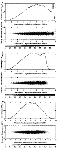
Figure 3. The three graphs in the left column are the normalized concentration functions $C_{\textsc{F}}(t,\cdot)/\max_{x}C_{\textsc{F}}(t,x)$ copied from Michalak and Kitanidis [10]. The three graphs in the right column are the normalized probability density functions $f^{\textsc{F}}_{\tilde{S}_{400}}(t,\cdot)/max_{x}f^{\textsc{F}}_{\tilde{S}_{400}}(t,x)$ given by the Fourier transformation in our paper. All graphs have $Pe=100,v=L=1,~{}R=2$. In the first row $Da_{I}=0.1,t^{*}=3.6$, in the second row $Da_{I}=0.33,t^{*}=3.2$, and in the last row $Da_{I}=1.0,t^{*}=3.0$.

Michalak and Kitanidis focus on the case that the solute starts in the free phase and the length of the initial solute is $L$, i.e., the initial distributions of the PDE’s (1) are given by

$$C_{\textsc{F}}(0,x)=\frac{1}{L}\textbf{1}_{[0,L]}(x),\quad C_{\textsc{A}}(0,x)=0.$$

So to make the comparison, we look at the probability density function $f_{\tilde{S}_{n}}^{\textsc{F}}(t,x)$ of

$$\tilde{S}^{\textsc{F}}_{n}(t)=S^{\textsc{F}}_{n}(t)+U_{L},$$

where $U_{L}$ is a uniformly distributed random variable over the interval $[0,L]$ (independent of $S_{n}^{\textsc{F}}(t)$). Michalak and Kitanidis point out that the double peaking behavior of the free concentration distribution is a function of the so called Damköhler number of the first kind $Da_{I}=\mu LR/v,$ where $R$ is the dimensionless retardation coefficient. They state that the timing of its appearance is controlled by the mass transfer rate and the retardation factor, i.e., the dimensionless time $t^{*}=\mu(R-1)t$. The so called Péclet number $Pe=vL/D$ is kept constant at a value of $100$. Recalling from Section 2 that $\lambda=\beta\mu=(R-1)\mu$ and $a=\lambda\Delta t,b=\mu\Delta t$, we translate these parameters into our paper as follows:

$$a=\frac{k(R-1)t}{n}=\frac{t^{*}}{n},\quad b=\frac{k\,t}{n}=\frac{t^{*}}{n(R-1)},\quad D=\frac{vL}{Pe},\quad\Delta t=\frac{t}{n}=\frac{t^{*}LR}{nv(R-1)Da_{I}}.$$

The graphs in the left column of Figure 3 are a copy of the graphs of the normalized aqueous concentration functions $C_{\textsc{F}}(t,\cdot)/\max_{x}C_{\textsc{F}}(t,x)$ (consisting of the free particles) in Michalak and Kitanidis [10] using simulations corresponding to different choices of the Damköhler number $Da_{I}$ and dimensionless time $t^{*}$. The three graphs in the right column of Figure 3 are the normalized density functions $f^{\textsc{F}}_{\tilde{S}_{400}}(t,\cdot)/\max_{x}f^{\textsc{F}}_{\tilde{S}_{400}}(t,x)$ calculated using Equation (20) corresponding to the same choice of $Da_{I}$ and $t^{*}$. The number $n$ is chosen large enough such that $\max{(a,b)}=\max{(\lambda\Delta t,\mu\Delta t)}\leq 0.01$. From Figure 3 it is obvious that our model gives a much better view at the double peaking phenomenon.

Figure 4. The three graphs are the probability density functions $f^{{\textsc{F}}}_{\tilde{S}_{400}}(t,\cdot)$ of $\tilde{S}_{400}^{\textsc{F}}(t)$. All graphs have $Pe=100,v=L=1,R=2,t^{*}=4.0$, and different Damköhler numbers.

Moreover, for each $t^{*}$, by a numerical calculation we can obtain upper bounds for $Da_{I}$ such that double peaks appear. For example, Figure 4 gives an intuition on how double peaks behave when $Da_{I}$ increases. We numerically calculated the upper bounds for $Da_{I}$ in Table $1$ corresponding to different dimensionless times $t^{*}$ with $R=2$. For example, when $t^{*}=2.0$ two peaks occur for all $Da_{I}>0$ until $Da_{I}=Da_{I}^{\max}=0.43$. Table $1$ suggests that double peaking is pronounced for $2\leq t^{*}\leq 5$, and almost dies out when $t^{*}<1.5$ or $t^{*}>10$.

Table 1. $R=2,Pe=100,v=1,L=1,n=400.$

$t^{*}$	1.5	2.0	2.5	3.0	3.5	4.0	4.5	5.0	6.0	7.0	8.0	9.0	10.0
$Da_{I}^{\max}$	0.12	0.43	1.45	1.42	0.73	0.45	0.30	0.21	0.11	0.07	0.04	0.02	0.02

10. Final remarks

We emphasize that the so called ‘random walk method’ or ‘particle tracking method’ first proposed by Kinzelbach [8] has a relation to our model, but has always been used as a simulation tool, to perform numerical experiments (for a recent example see [1]). In fact it is shown in [15] for the first time that if one takes an appropriate limit (in a similar way as in [4]), then the Fokker-Planck equations of an extended version of our simple model to a Markov chain which also involves discrete steps in space, yield the partial differential equations (1) in Section 2.

Finally we mention that our computations yield the following. If one starts in the stationary distribution, i.e., $\nu=(\pi_{\textsc{F}},\pi_{\textsc{A}})$, then $\varepsilon_{{\textsc{F}}}=\varepsilon_{{\textsc{A}}}=0$. Substituting

$$\varepsilon_{{\textsc{F}}}=0,\quad\pi_{\textsc{F}}=\frac{\mu}{\lambda+\mu},\quad\pi_{\textsc{A}}=\frac{\lambda}{\lambda+\mu}$$

in Proposition 8.1, we obtain

$$\begin{split}{\rm Var}_{\nu}\!\left(S(t)\right)=&\frac{2D\mu}{\lambda+\mu}t+\frac{2\mu\lambda}{(\lambda+\mu)^{3}}v^{2}t-\frac{2\mu\lambda}{(\lambda+\mu)^{4}}v^{2}\Big{(}1-\exp{\big{(}-(\lambda+\mu)t\big{)}}\Big{)}.\end{split}$$

We then recuperate a (more general and more detailed) version of the main result of Gut and Ahlberg ([7], p.251).

References

[1]
David A. Benson and Mark M. Meerschaert.
A simple and efficient random walk solution of multi-rate
mobile/immobile mass transport equations.
Advances in Water Resources, 32(4):532–539, 2009.
[2]
Patrick Billingsley.
Probability and measure,.
Wiley Series in Probability and Mathematical Statistics. John Wiley
& Sons Inc., New York, third edition, 1995.
A Wiley-Interscience Publication.
[3]
J. N. Darroch and K. W. Morris.
Passage-time generating functions for continuous-time finite Markov
chains.
J. Appl. Probability, 5:414–426, 1968.
[4]
H. G. Dehling, A. C. Hoffmann, and H. W. Stuut.
Stochastic models for transport in a fluidized bed.
SIAM J. Appl. Math., 60(1):337–358, 2000.
[5]
Michel Dekking and DeRong Kong.
Multimodality of the Markov binomial distribution.
arXiv:1102.3613v1, 2011.
[6]
R. Durrett.
Probability: Theory and Examples,.
Cambridge University Press, Cambridge, fourth edition, 2010.
[7]
A. Gut and P. Ahlberg.
On the theory of chromatography based upon renewal theory and a
central limit theorem for randomly iterated indexed partial sums of random
variables.
Chemica Scripta, 18(5):248–255, 1981.
[8]
W. Kinzelbach.
The random walk method in pollutant transport simulation.
In E. Custodio, editor, Groundwater Flow and Quality Modelling,
NATO ASI Series C: Mathematical and Physical Sciences vol. 224, pages
227–245, 1988.
[9]
F. T. Lindstroml and M.N.L. Narasimham.
Mathematical theory of a kinetic model for dispersion of previously
distributed chemicals in a sorbing porous medium.
SIAM J. Appl. Math., 24(4):496–510, 1973.
[10]
A.M. Michalak and Peter K. Kitanidis.
Macroscopic behavior and random-walk particle tracking of kinetically
sorbing solutes.
Water Resources Research, 36(8):2133–2146, 2000.
[11]
E. Omey, J. Santos, and S. Van Gulck.
A Markov-binomial distribution.
Appl. Anal. Discrete Math., 2(1):38–50, 2008.
[12]
P. J. Pedler.
Occupation times for two state Markov chains.
J. Appl. Probability, 8:381–390, 1971.
[13]
S. M. Ross.
Introduction to probability models,.
Academic Press/Elsevier Inc., USA, ninth edition, 2007.
[14]
J. L. Schiff.
The Laplace transform: theory and application.
Springer-Verlag, New York, 1991.
[15]
G. Uffink, A. Elfeki, M. Dekking, J. Bruining, and C. Kraaikamp.
Understanding the non-Gaussianity of reactive transport; from
particle dynamics to PDE’s.
arXiv:1101.2510v1, 2010.
[16]
R. Viveros, K. Balasubramanian, and N. Balakrishnan.
Binomial and negative binomial analogues under correlated Bernoulli
trials.
The American Statistician, 48:243–247, 1994.