Future cosmological evolution in $f(R)$ gravity using two equations of state parameters

Abstract

We investigate the issues of future oscillations around the phantom divide for $f(R)$ gravity. For this purpose, we introduce two types of energy density and pressure arisen from the $f(R)$-higher order curvature terms. One has the conventional energy density and pressure even in the beginning of the Jordan frame, whose continuity equation provides the native equation of state $w_{\rm DE}$. On the other hand, the other has the different forms of energy density and pressure which do not obviously satisfy the continuity equation. This needs to introduce the effective equation of state $w_{\rm eff}$ to describe the $f(R)$-fluid, in addition to the native equation of state $\tilde{w}_{\rm DE}$. We confirm that future oscillations around the phantom divide occur in $f(R)$ gravities by introducing two types of equations of state. Finally, we point out that the singularity appears ar $x=x_{c}$ because the stability condition of $f(R)$ gravity violates.

I Introduction

Supernova type Ia(SUN Ia) observations has shown that our universe is accelerating SN . Also cosmic microwave background radiation Wmap , large scale structure lss , and weak lensing wl have indicated that the universe has been undergoing an accelerating phase since the recent past. The standard model of ${\rm\Lambda}$CDM enables to explain these observational results within observational error bound. However, this model suffers from the cosmological constant problem and thus, one needs to find another model. Up to now, the $f(R)$-gravity as a modified gravity model remains a promising model to explain the present accelerating universe cst ; NO ; sf ; NOuh ; FT . $f(R)$ gravities can be considered as Einstein gravity (massless graviton) with an additional scalar. For example, it was shown that the metric-$f(R)$ gravity is equivalent to the $\omega_{\rm BD}=0$ Brans-Dicke (BD) theory with the potential FT . Although the equivalence principle test in the solar system imposes a strong constraint on $f(R)$ gravities, they may not be automatically ruled out if the Chameleon mechanism is introduced to resolve it in the Einstein frame. It was shown that the equivalence principle test allows $f(R)$ gravity models that are indistinguishable from the ${\rm\Lambda}$CDM model in the background universe evolution PS .

In order to point out the difference between ${\rm\Lambda}$CDM and $f(R)$ gravity, it is necessary to introduce the equation of state parameter $w_{\rm DE}$. Working with the $f(R)$-gravity action in the Jordan frame Jordan , one has to use the different energy density and pressure $(\tilde{\rho}_{\rm DE},\tilde{p}_{\rm DE})$ in compared to $(\rho_{\rm DE},p_{\rm DE})$ in the Einstein-like frame BGL ; MSY . This corresponds to the scalar-tensor (Brans-Dicke) theory in the Jordan frame LKM . In the Einstein-like frame, one needs only the native equation of state $w_{\rm DE}=p_{\rm DE}/\rho_{\rm DE}$ as in the scalar-tensor (quintessence model) theory, while one requires two equations of states: ${\tilde{w}}_{\rm DE}={\tilde{p}}_{\rm DE}/{\tilde{\rho}}_{\rm DE}$ and the effective equation of state $w_{\rm eff}$ ZP1 because of non-minimal coupling of scalar to the gravity. It is worth noting that there is an essential difference between Einstein-like and Einstein frames because the latter is recovered from the conformal transformation in Jordan frame FT ; PHSS . For the holographic dark energy model, two of authors have clarified that although there is a phantom phase when using the native equation of state WGA , there is no phantom phase when using the effective equation of state KLM ; KLMb .

Recently, there were a few of important works which explain the oscillation around the future de Sitter solution with $w_{\rm dS}=-1$ using $f(R)$-gravity BGL and its Brans-Dicke theory LKM . Interestingly, the authors in MSY have shown that the number of phantom divide crossings are infinite when using the Ricci scalar perturbation, which is confirmed by analytical condition and numerical way.

In this work, we focus on the issues of future oscillations around the phantom divide for $f(R)$ gravity. In order to confirm the appearance of future oscillations around the phantom divide $w_{\rm dS}=-1$, we introduce two types of equation of states $w_{\rm DE}(\tilde{w}_{\rm DE})$ and $w_{\rm eff}$ arisen from the $f(R)$-fluid. We clarify the difference between two different sets of energy density and pressure by observing the “negative and effective” equations of state. Finally, we point out that the singularity appears at $x=x_{c}$ because the stability condition of $f(R)$ gravity violates when $F^{\prime}=f^{\prime\prime}=0$ at the certain point $x=x_{c}$.

II Future volution with $f(R)$-fluid in Einstein-like frame

We start from the action of $f(R)$ gravity with matter as

$$I=\frac{1}{2\kappa^{2}}\int d^{4}x\sqrt{-g}f(R)+I_{\rm m}(g_{\mu\nu},\psi_{\rm m}),$$ (1)

where $f(R)$ is a function of Ricci scalar $R$ with $\kappa^{2}=8\pi G$ and $I_{\rm m}$ is the action for matter which is assumed to be minimally coupled to gravity. Here the action $I$ is initially written in Jordan frame and $\psi_{\rm m}$ denotes matters. Taking the variation of the action (1) with respect to metric $g_{\mu\nu}$, one obtains

$$FG_{\mu\nu}=\kappa^{2}T_{\mu\nu}^{\rm(m)}-\frac{1}{2}g_{\mu\nu}\left(FR-f\right)+\nabla_{\mu}\nabla_{\nu}F-g_{\mu\nu}\nabla^{2}F,$$ (2)

where $G_{\mu\nu}=R_{\mu\nu}-\frac{g_{\mu\nu}}{2}R$ is the Einstein tensor and $F(R)=f^{\prime}(R)$. Assuming the flat Friedmann-Roberston-Walker (FRW) universe

$$ds^{2}_{\rm FRW}=-dt^{2}+a^{2}(t)\Big{(}dr^{2}+r^{2}d\Omega^{2}_{2}\Big{)}$$ (3)

with $a(t)$ is the scale factor, we obtain the two Friedmann equations from (2):

$$3FH^{2} = \kappa^{2}\rho_{\rm M}+\frac{1}{2}\left(FR-f\right)-3H{\dot{F}},$$ (4)

$$-2F{\dot{H}} = \kappa^{2}\left(\rho_{\rm M}+p_{\rm M}\right)+{\ddot{F}}-H{\dot{F}},$$ (5)

where $H={\dot{a}}/a$ is the Hubble parameter, the overdot denotes the derivative with respect to the cosmic time $t$, and $\rho_{\rm M}$ and $p_{\rm M}$ are the energy density and pressure of all perfect fluid-type matter, respectively. On the other hand, the scalar curvature $R$ defined by

$$R=6\left({\dot{H}}+2H^{2}\right)$$ (6)

plays an independent role in the cosmological evolution because we are working with $f(R)$-fluid. For our purpose, we introduce the new variable $x=\ln a$, then (4) and (6) take the forms

$$H^{2} = \left(F-1\right)\left(H\frac{dH}{dx}+H^{2}\right)-\frac{1}{6}\left(f-R\right)-H^{2}F^{\prime}\frac{dR}{dx}+\frac{\kappa^{2}\rho_{m}^{0}e^{-3x}}{3}+\frac{\kappa^{2}\rho_{m}^{0}e^{-4x}}{3}\chi,$$ (7)

$$R = 6\left(H\frac{dH}{dx}+2H^{2}\right),$$ (8)

where $\rho_{m}^{0}$ is the current density of cold dark matter (CDM) and $\chi=\rho_{r}^{0}/\rho_{m}^{0}\simeq 3.1\times 10^{-4}$ is the current density ratio of radiation and dark matter. Regarding (7) as the evolution equation, we rewrite it as a compact form

$$H^{2}=\frac{\kappa^{2}}{3}\left(\rho_{\rm DE}+\rho_{\rm m}+\rho_{\rm r}\right),$$ (9)

where $\rho_{\rm DE}$, $\rho_{\rm m}$, and $\rho_{\rm r}$ represent dark energy, dark matter and radiation, respectively. Comparing (7) with (9) leads to a definition of dark energy density arisen from the $f(R)$-gravity BGL ; MSY

$$\rho_{\rm DE}=\frac{3}{\kappa^{2}}\Bigg{[}\left(F-1\right)\left(H\frac{dH}{dx}+H^{2}\right)-\frac{1}{6}\left(f-R\right)-H^{2}F^{\prime}\frac{dR}{dx}\Bigg{]}.$$ (10)

This dark energy density satisfies the conservation law as

$${\dot{\rho}}_{\rm DE}+3H\left(1+w_{\rm DE}\right)\rho_{\rm DE}=0$$ (11)

with the native equation of state

$$w_{\rm DE}=\frac{p_{\rm DE}}{\rho_{\rm DE}}.$$ (12)

Importantly, we observe that even starting with the $f(R)$ gravity action in the Jordan frame, we have manipulated it so that the Einstein equation (2) is rewritten effectively as

$$G_{\mu\nu}=G_{\mu\nu}(1-F)+\kappa^{2}T_{\mu\nu}^{\rm(m)}-\frac{1}{2}g_{\mu\nu}\left(FR-f\right)+\nabla_{\mu}\nabla_{\nu}F-g_{\mu\nu}\nabla^{2}F,$$ (13)

to derive (7) and (9) for obtaining the standard dark energy $\rho_{\rm DE}$ and pressure $p_{\rm DE}$. Hence we call the solution to (9) with (10) as cosmological evolution with $f(R)$-fluid in Einstein-like frame.

In order to solve (7) and (8) simultaneously, we define the convenient variables call the reduced Ricci scalar $r$ and the present matter-density parameter $\Omega_{\rm m}^{0}$

$$r\equiv\frac{R}{6H^{2}},\ \ \ \Omega_{\rm m}^{0}\equiv\frac{\rho_{\rm m}^{0}}{\rho_{\rm crit}^{0}}=\frac{\kappa^{2}\rho_{\rm m}^{0}}{3H_{0}^{2}},$$ (14)

and density parameters

$$\Omega_{\rm m}=\frac{\rho_{\rm m}}{\rho_{\rm crit}},~{}~{}\Omega_{\rm r}=\frac{\rho_{\rm r}}{\rho_{\rm crit}},~{}~{}\Omega_{\rm DE}=1-\Omega_{\rm m}-\Omega_{\rm r}.$$ (15)

Then two equations (7) and (8) can be written four equations in terms of new variables

$$\frac{d\Omega_{\rm m}}{dx} = -(2r-1)\Omega_{\rm m},$$ (16)

$$\frac{d\Omega_{\rm r}}{dx} = -2r\Omega_{\rm r},$$ (17)

$$\frac{dr}{dx} = -2r(r-2)+\frac{F}{6H^{2}F^{\prime}}\left\{-1+\frac{\Omega_{\rm m}+\Omega_{\rm r}}{F}+r-\frac{1}{6H^{2}}\frac{f}{F}\right\},$$ (18)

$$\frac{dH}{dx} = (r-2)H.$$ (19)

Considering

$$\frac{d\Omega_{\rm DE}}{dx}=-2\Omega_{\rm DE}(r-2)+\frac{\kappa^{2}}{3H^{2}}\frac{d\rho_{\rm DE}}{dx},$$ (20)

one obtains the native equation of states as functions of $r$ and density parameters as

$$w_{\rm DE}(r,\Omega_{\rm m},\Omega_{\rm r})=-1-\frac{2r-4+3\Omega_{\rm m}+4\Omega_{\rm r}}{3(1-\Omega_{\rm m}-\Omega_{\rm r})}.$$ (21)

At this stage, we wish to comment on the tilde-definition for density parameters used in Ref. BGL

$${\tilde{\Omega}}_{\rm m} = \frac{\rho_{\rm m}}{\rho_{\rm crit}^{0}}=\Omega_{\rm m}h^{2},$$ (22)

$${\tilde{\Omega}}_{\rm r} = \frac{\rho_{\rm m}}{\rho_{\rm crit}^{0}}=\Omega_{\rm r}h^{2},$$ (23)

$${\tilde{\Omega}}_{\rm DE} = \frac{\rho_{\rm m}}{\rho_{\rm crit}^{0}}=\Omega_{\rm DE}h^{2},$$ (24)

which are clearly different from our definition by $h^{2}$ factor, which is defined as $h(x)=H(x)/H_{0}$. Finally, we mention that the initial conditions for $\Omega_{\rm m},\Omega_{\rm r},r$ and $H$ are given by

$$\Omega_{\rm m}(0)=\Omega_{\rm m}^{0},~{}~{}\Omega_{\rm r}(0)=\chi\Omega_{\rm m}^{0},~{}~{}r(0)=2+h_{1},~{}~{}H(0)=1,$$ (25)

where $h_{1}$ is the time derivative of $H$ at the present time $t=0$ with $a(0)=1$. Then, $x\in[-\infty,\infty]$ with $x=0$ at the present time. We note that $h_{1}$ is related to deceleration parameter $q$ as

$$h_{1}=-\left(1+q\right)$$ (26)

with

$$q\equiv-\frac{{\ddot{a}}{a}}{{\dot{a}}^{2}}=-\frac{{\ddot{a}}}{a}\frac{1}{H^{2}}=-\left.\frac{1}{H}\frac{dH}{dx}\right|_{0}-1=-h_{1}-1.$$ (27)

Now we study the cosmological evolution by choosing four specific models of $f(R)$-gravity with the native equation of state $w_{\rm DE}$ only.

II.1 Cosmological constant

For cosmological constant case, the function $f(R)$ is simply given by

$$f(R)=R+\Lambda.$$ (28)

In this case one cannot use (18) because of $F^{\prime}(R)=f^{\prime\prime}(R)=0$, but other equations are being used to derive the solutions. Equation (7) becomes

$$H^{2}=-\frac{\Lambda}{6}+H_{0}^{2}\Omega_{\rm m}^{0}\left(e^{-3x}+\chi e^{-4x}\right).$$ (29)

Differentiating this equation with respect to $x$, we get

$$2H\frac{dH}{dx}=H_{0}^{2}\Omega_{\rm m}^{0}\left(-3e^{-3x}-4\chi e^{-4x}\right).$$ (30)

Plugging this into the definition of $r$, one gets

$$r=2-\frac{3}{2}\Omega_{\rm m}-2\Omega_{\rm r}.$$ (31)

Hence, the relevant equation is just

$$\frac{dr}{dx}=\frac{3}{2}(2r-1)\Omega_{\rm m}+4r\Omega_{\rm r}$$ (32)

with $w_{\rm DE}=-1$. Fig. 1 depicts the evolution for the cosmological constant like the ${\rm\Lambda}$CDM without future oscillations around the phantom divide $w_{\rm DE}=w_{\rm dS}=-1$ .

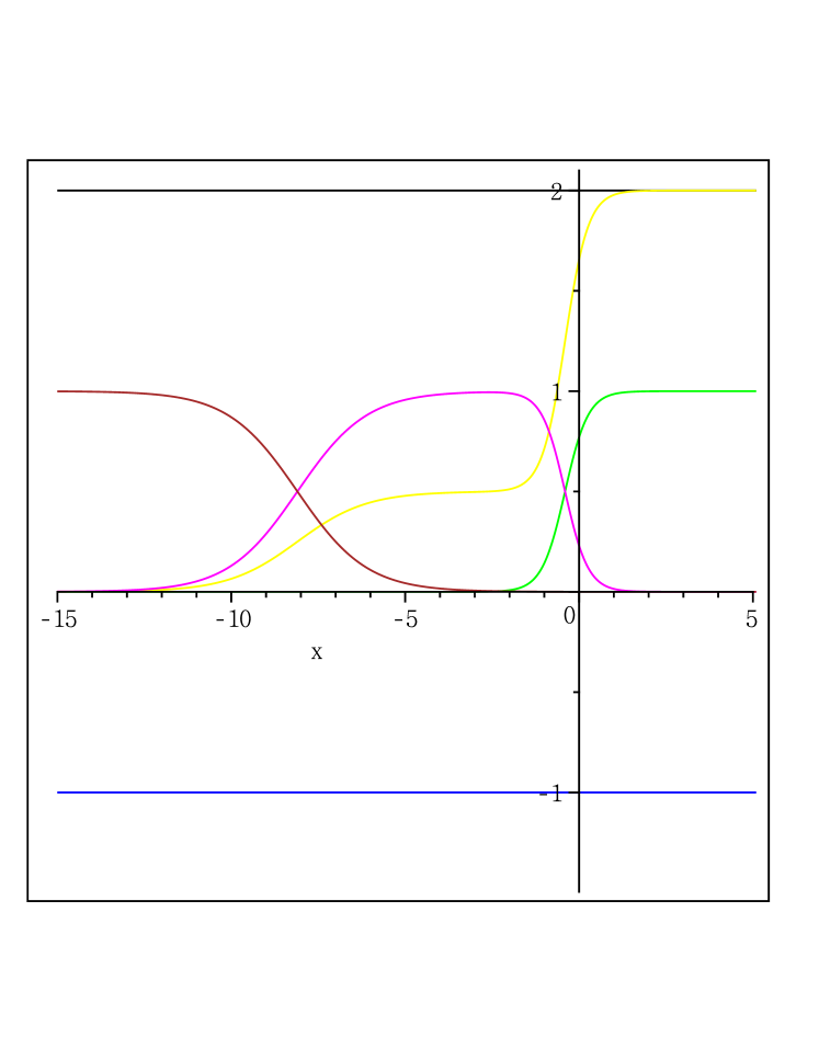
Figure 1: Time evolution of cosmological parameters for cosmological constant case: $w_{\rm DE}$(blue), $\Omega_{\rm DE}$(green), $\Omega_{\rm m}$(magenta), $\Omega_{\rm r}$(brown), and $r$(yellow) for $\Omega_{\rm m}^{0}=0.23$ and $\chi=3.04\times 10^{-4},h_{1}=-(\frac{3}{2}+\frac{\chi}{2})\Omega_{\rm m}^{0}$.

We point out that the reduced Ricci scalar $r$ takes the value of $r_{\rm dS}=2$ because of $R_{\rm dS}=12H^{2}$ for the de Sitter spacetimes.

II.2 Power-law gravity

When $f(R)$ takes the power-law form

$$f(R)=R+f_{0}R^{\alpha},$$ (33)

Its derivatives with respect to $R$ are given by

$$F(R)=1+\alpha f_{0}R^{\alpha-1},~{}~{}F^{\prime}(R)=\alpha(\alpha-1)f_{0}R^{\alpha-2}.$$ (34)

$w_{\rm DE}$ and $r$ in Figs. 2 and 3 represent the future oscillations around the phantom divide for $\alpha=1/2$ and 1/3, respectively but they do not show past oscillations around the phantom divide.

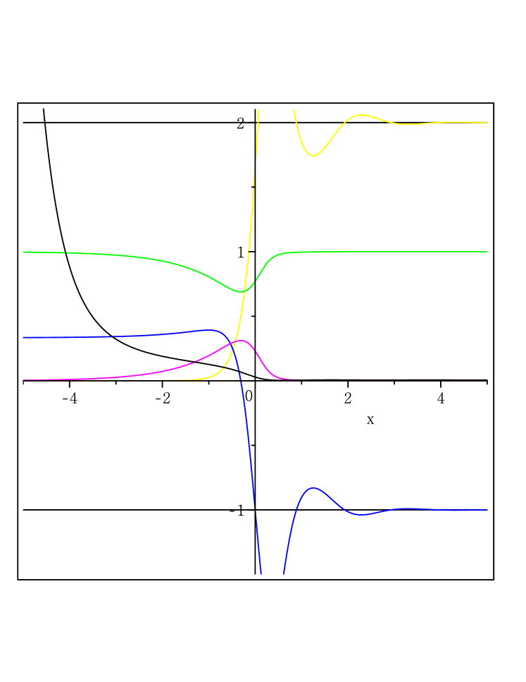
Figure 2: Time evolution of cosmological parameters for power-law case: $w_{\rm DE}$(blue), $\Omega_{\rm DE}$(green), $\Omega_{\rm m}$(magenta), $\Omega_{\rm r}$(brown), $r$(yellow), and $F^{\prime}$ (black) for ${f}_{0}=-3.6,\alpha=1/2,\Omega_{\rm m}^{0}=0.23,\chi=3.04\times 10^{-4},h_{1}=-(\frac{3}{2}+\frac{\chi}{2})\Omega_{\rm m}^{0}$.

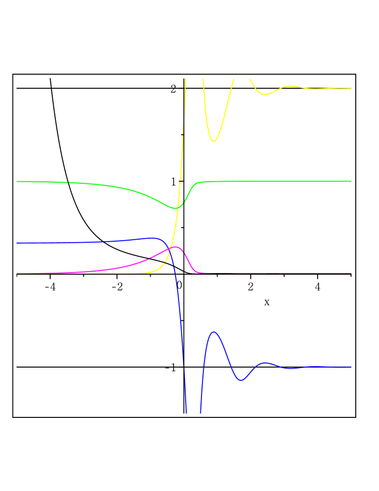
Figure 3: Time evolution of cosmological parameters for power-law case: $w_{\rm DE}$(blue), $\Omega_{\rm DE}$(green), $\Omega_{\rm m}$(magenta), $\Omega_{\rm r}$(brown), $r$(yellow), and $F^{\prime}$ (black) for ${f}_{0}=-6.5,\alpha=1/3,\Omega_{\rm m}^{0}=0.23,\chi=3.04\times 10^{-4},h_{1}=-(\frac{3}{2}+\frac{\chi}{2})\Omega_{\rm m}^{0}$.

II.3 Exponential gravity

Now we wish to apply the result of previous sub-sections to an exponential gravity. Firstly, when the function $f(R)$ is given by

$$f(R)=R-\beta R_{s}\left(1-e^{-R/R_{s}}\right),$$ (35)

its derivatives with respect to $R$ are given by

$$F(R)=1-\beta e^{-R/R_{s}},~{}~{}F^{\prime}(R)=\frac{\beta}{R_{s}}e^{-R/R_{s}}.$$ (36)

Fig. 4 indicates no the appearance of future (past) oscillations around the phantom divide for a given parameter $R_{s}=-0.05$ and $\beta=1.1$ which is the same results found in  BGLe . We note that $F^{\prime}$ does not appear in Fig. 4 because its value is extremely large as $10^{87}$.

Figure 4: Time evolution of cosmological parameters for an exponential case: $w_{\rm DE}$(blue), $\Omega_{\rm DE}$(green), $\Omega_{\rm m}$(magenta), $\Omega_{\rm r}$(brown), $r$(yellow), and $F^{\prime}$ (black) for $R_{s}=-0.05,\beta=1.1,\Omega_{\rm m}^{0}=0.23,\chi=3.04\times 10^{-4},h_{1}=-(\frac{3}{2}+\frac{\chi}{2})\Omega_{\rm m}^{0}$.

II.4 Hu and Sawicki model

The Hu and Sawicki model takes the form

$$f(R)=R-\mu R_{c}\left[1-\left(1+\frac{R^{2}}{R_{c}^{2}}\right)^{-n}\right].$$ (37)

Its derivatives with respect to $R$ are given by

$$F(R) = 1-2\mu n\frac{R}{R_{c}}\left(1+\frac{R^{2}}{R_{c}^{2}}\right)^{-(n+1)},$$ (38)

$$F^{\prime}(R) = -\frac{2\mu n}{R_{c}}\left[1-(2n+1)\frac{R^{2}}{R_{c}^{2}}\right]\left(1+\frac{R^{2}}{R_{c}^{2}}\right)^{-(n+2)}.$$ (39)

Fig. 5 shows that future oscillations around the phantom divide $w_{\rm dS}=-1$ appears for $R_{c}=-1.0,~{}\mu=-1.5,$ and $n=2$, but there is no evolution toward the past direction from $x_{c}=0$. Similarly, there are future oscillations around $r_{\rm dS}=2$ for the reduced Ricci scalar $r$. We will explain why the evolution to the past is not allowed in the Hu and Sawicki model in section IV.

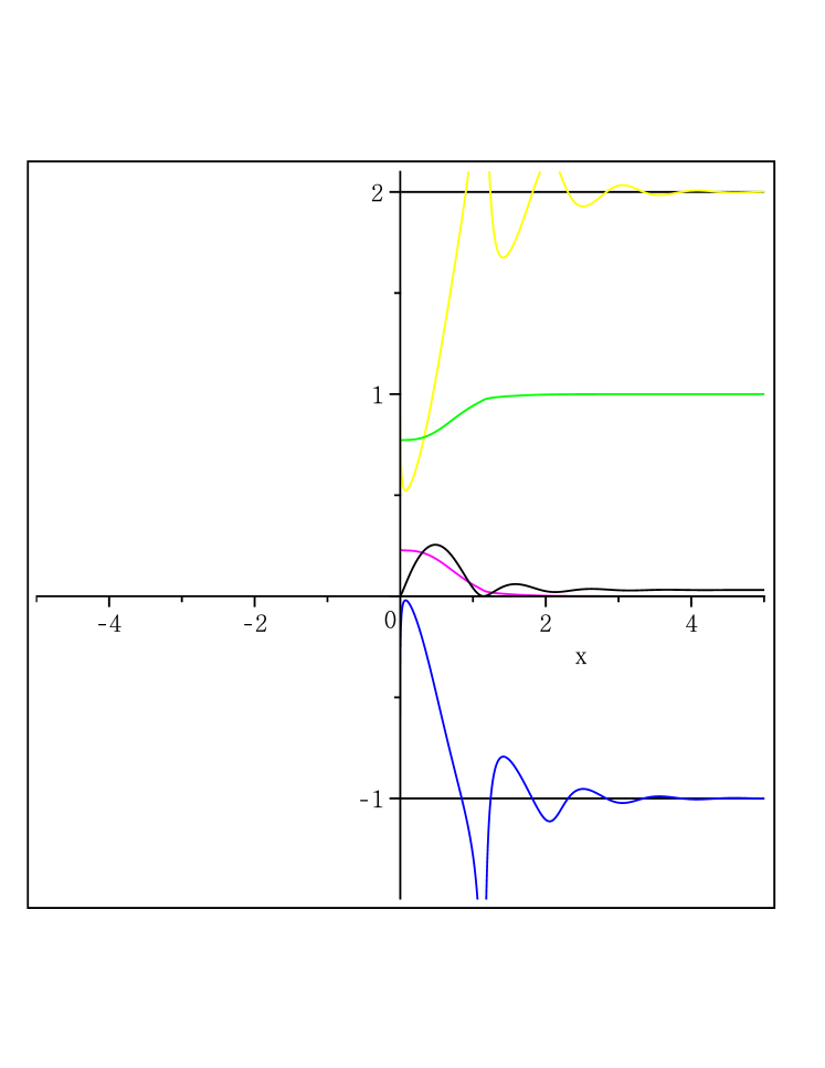
Figure 5: Time evolution of cosmological parameters for the Hu and Sawicki model: $w_{\rm DE}$(blue), $\Omega_{\rm DE}$(green), $\Omega_{\rm m}$(magenta), $\Omega_{\rm r}$(brown), $r$(yellow), and $F^{\prime}$ (black) for $R_{c}=-1.0,\mu=-1.5,n=2,\Omega_{\rm m}^{0}=0.23,\chi=3.04\times 10^{-4},h_{1}=-(\frac{3}{2}+\frac{\chi}{2})\Omega_{\rm m}^{0}$.

III Cosmological evolution in Jordan frame

In this section we derive evolution equations in Jordan frame without manipulation. From equations (4) and (5), we have

$$H^{2} = \frac{1}{3F}\Bigg{[}\kappa^{2}\rho_{\rm M}+\frac{1}{2}\left(FR-f\right)-3H{\dot{F}}\Bigg{]},$$ (40)

$$-{\dot{H}} = \frac{1}{2F}\Bigg{[}\kappa^{2}\left(\rho_{\rm M}+p_{\rm M}\right)+{\ddot{F}}-H{\dot{F}}\Bigg{]},$$ (41)

Introducing the reduced Ricci scalar $r$

$$r=\frac{R}{6H^{2}},$$ (42)

we can obtain an important relation

$$\frac{F^{\prime}}{F}\frac{dR}{dx} = -1+\Omega_{\rm m}+\Omega_{\rm r}+\frac{1}{6H^{2}}\left(R-\frac{f}{F}\right),$$ (43)

In this case, we read off energy density and pressure of the dark energy component from (40) and (41) as Jordan

$$\tilde{\rho}_{\rm DE} = \frac{1}{\kappa^{2}F}\left\{\frac{FR-f}{2}-3H{\dot{F}}\right\},$$ (44)

$$\tilde{p}_{\rm DE} = \frac{1}{\kappa^{2}F}\left\{-\frac{FR-f}{2}+2H{\dot{F}}+{\ddot{F}}\right\}.$$ (45)

Rewriting the Einstein equation (2) as

$$G_{\mu\nu}=\kappa^{2}\frac{T_{\mu\nu}^{\rm(m)}}{F}+\kappa^{2}T_{\mu\nu}^{\rm DE},$$ (46)

we obtain the non-conservation of continuity relation by requiring the Bianchi idensity

$${\dot{\tilde{\rho}}}_{\rm DE}+3H\left(\tilde{\rho}_{\rm DE}+\tilde{p}_{\rm DE}\right)=\frac{\dot{F}}{F^{2}}\rho_{\rm M}.$$ (47)

Because of the non-zero coupling term between $\rho_{M}$ and $\frac{\dot{F}}{F^{2}}$, we must define an “effective” equation of state for $f(R)$-fluid

$$w_{\rm eff}={\tilde{w}}_{\rm DE}-\frac{-1+\Omega_{\rm m}+\Omega_{\rm r}+r-\frac{f}{6H^{2}F}}{3}\Bigg{[}\frac{\Omega_{\rm m}+\Omega_{\rm r}}{1-\Omega_{\rm m}-\Omega_{\rm r}}\Bigg{]},$$ (48)

with the native equation of state $\tilde{w}_{\rm DE}=\tilde{p}_{\rm DE}/\tilde{\rho}_{\rm DE}$. This is similar to the Brans-Dicke theory approach KLM ; LKM . Defining density parameters newly as

$$\Omega_{\rm m}=\frac{\kappa^{2}}{3H^{2}}\frac{\rho_{\rm m}}{F},\,\,\Omega_{\rm r}=\frac{\kappa^{2}}{3H^{2}}\frac{\rho_{\rm r}}{F},\,\,\Omega_{\rm DE}=\frac{\kappa^{2}}{3H^{2}}\tilde{\rho}_{\rm DE},$$ (49)

relevant quantities are expressed by

$$R = 6H^{2}r,$$ (50)

$$\tilde{\rho}_{\rm DE} = \frac{3H^{2}}{\kappa^{2}}\left\{1-\Omega_{\rm m}-\Omega_{\rm r}\right\},$$ (51)

$$\tilde{p}_{\rm DE} = \frac{3H^{2}}{\kappa^{2}}\left\{-1-\frac{1}{3}\Omega_{\rm r}-\frac{2}{3}(r-2)\right\}.$$ (52)

Insereting these into the definition of native equation of state, one gets

$${\tilde{w}}_{\rm DE}=-1-\frac{2r-4+3\Omega_{\rm m}+4\Omega_{\rm r}}{3(1-\Omega_{\rm m}-\Omega_{\rm r})},$$ (53)

which is the same as Eq. (21) but their forms of $\Omega_{\rm m}$ and $\Omega_{\rm m}$ are different from those in (21).

Four equations to be solved become

$$\frac{d\Omega_{\rm m}}{dx} = -\left(2r-2+\Omega_{\rm m}+\Omega_{\rm r}+r-\frac{f}{6H^{2}F}\right)\Omega_{\rm m},$$ (54)

$$\frac{d\Omega_{\rm r}}{dx} = -\left(2r-1+\Omega_{\rm m}+\Omega_{\rm r}+r-\frac{f}{6H^{2}F}\right)\Omega_{\rm r},$$ (55)

$$\frac{dr}{dx} = -2r(r-2)+\frac{F}{6H^{2}F^{\prime}}\left(-1+\Omega_{\rm m}+\Omega_{\rm r}+r-\frac{f}{6H^{2}F}\right),$$ (56)

$$\frac{dH}{dx} = (r-2)H.$$ (57)

Finally, we have to consider the initial conditions

$$H(0)=H_{0}=1,\,\,\Omega_{\rm r}(0)=\chi\Omega_{\rm m}^{0},\,\,r_{0}=2+h_{1},h_{1}=-(1+q),$$ (58)

with $q$ the deceleration parameter.

Now we solve the above four differential equations together with initial conditions by selecting four interesting models.

III.1 $f(R)=R+\Lambda$ case

In this case, we cannot use Eq. (56), which is valid only for $F^{\prime}\neq 0$. In this case, $r$ is given by

$$r=2-\frac{3}{2}\Omega_{\rm m}-2\Omega_{\rm r}.$$ (59)

Hence the density and pressure of $f(R)$-fluid are given

$$\tilde{\rho}_{\rm DE} = \frac{3H^{2}}{\kappa^{2}}\left(1-\Omega_{\rm m}-\Omega_{\rm r}\right),$$ (60)

$$\tilde{p}_{\rm DE} = \frac{3H^{2}}{\kappa^{2}}\left(-1+\Omega_{\rm m}+\Omega_{\rm r}\right).$$ (61)

Therefore, we have $\tilde{w}_{\rm DE}=-1=w_{\rm eff}$.

$$\frac{d\Omega_{\rm m}}{dx} = -\left(2r-1\right)\Omega_{\rm m},$$ (62)

$$\frac{d\Omega_{\rm r}}{dx} = -2r\Omega_{\rm r},$$ (63)

$$r = -\frac{3}{2}\Omega_{\rm m}-2\Omega_{\rm r},$$ (64)

$$\frac{dH}{dx} = (r-2)H.$$ (65)

Note that these equations are exactly the same as the previous section. Fig. 6 shows the same result that the future oscillations around the phantom divide does not appear in the Jordan frame.

Figure 6: Time evolution of cosmological parameters for cosmological constant case, $w_{\rm DE}$(blue), $\Omega_{\rm DE}$(green), $\Omega_{\rm m}$(magenta), $\Omega_{\rm r}$(brown), $r$(yellow), for $\Omega_{\rm m}^{0}=0.23$ and $\chi=3.04\times 10^{-4},h_{1}=-(\frac{3}{2}+\frac{\chi}{2})\Omega_{\rm m}^{0}$.

We observe that the deceleration parameter $q$ is fixed by the relation

$$1+q=-\left(\frac{3}{2}+\frac{\chi}{2}\right)\Omega_{\rm m}^{0}.$$ (66)

For $\Omega_{\rm DE}^{0}=0.77,\Omega_{\rm m}^{0}=0.23,\chi=3.1\times 10^{-4}$, it gives us $q=-0.6549643500$ and $h_{1}=-0.3451398400$.

III.2 $f(R)=R+f_{0}R^{\alpha}$ case

In this case, $F(R)$ is given

$$F(R)=1+\alpha f_{0}R^{\alpha-1}.$$ (67)

Its derivatives with respect to $R$ are given by

$$F(R) = 1+\alpha f_{0}R^{\alpha-1},$$ (68)

$$F^{\prime}(R) = \alpha(\alpha-1)f_{0}R^{\alpha-2}.$$ (69)

Figs. 7 and 8 show future oscillations around the phantom divide using $\tilde{w}_{\rm DE}$ as in Figs. 2 and 3 but the past evolution is terminated near $x_{c}\simeq-2.4$ for $\alpha=1/2$ and $x_{c}\simeq 3.4$ for $\alpha=1/3$. Also, the reduced Ricci scalar $r$ shows similar oscillating behaviors. This indicates a violation of stability condition as will explain in section IV. We confirm the appearance of future oscillations around the phantom using the effective equation of state $w_{\rm eff}$.

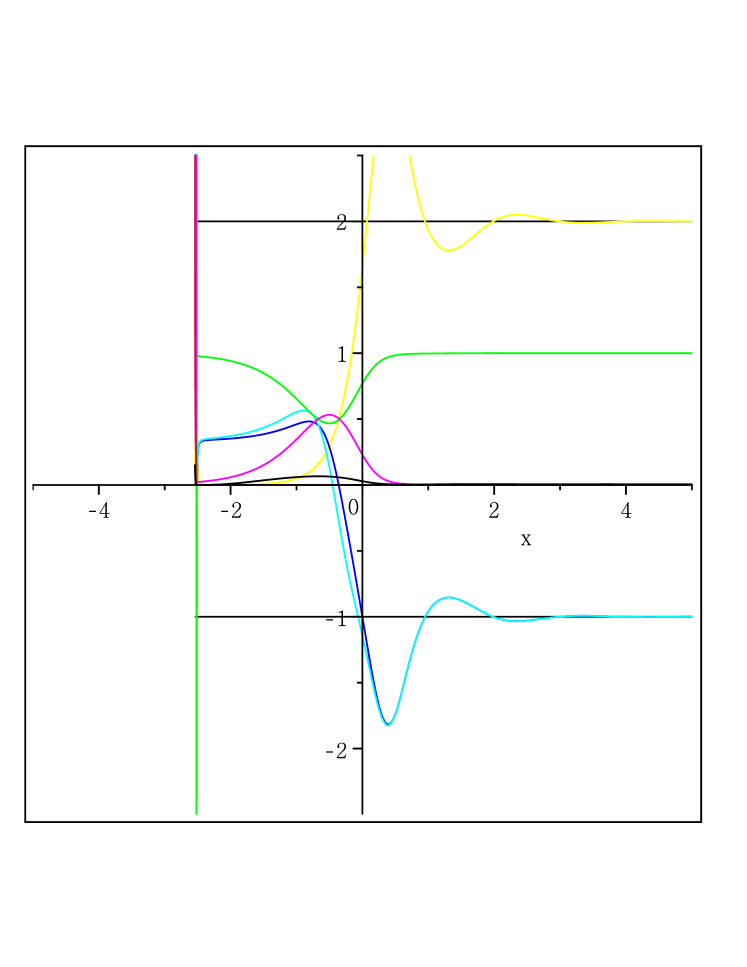
Figure 7: Time evolution of cosmological parameters for power-law case in Jordan frame: $\tilde{w}_{\rm DE}$(blue), $w_{\rm eff}$(cyan), $\Omega_{\rm DE}$(green), $\Omega_{\rm m}$(magenta), $\Omega_{\rm r}$(brown), $r$(yellow), and $F^{\prime}$ (black) for ${f}_{0}=-3.6,\alpha=1/2,\Omega_{\rm m}^{0}=0.23,\chi=3.04\times 10^{-4},h_{1}=-(\frac{3}{2}+\frac{\chi}{2})\Omega_{\rm m}^{0}$.

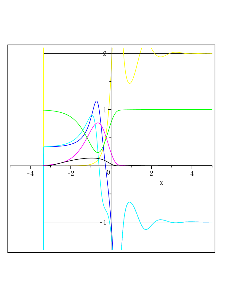
Figure 8: Time evolution of cosmological parameters for power-law case in Jordan frame: $\tilde{w}_{\rm DE}$(blue), $w_{\rm eff}$(cyan), $\Omega_{\rm DE}$(green), $\Omega_{\rm m}$(magenta), $\Omega_{\rm r}$(brown), $r$(yellow), and $F^{\prime}$ (black) for ${f}_{0}=-6.5,\alpha=1/3,\Omega_{\rm m}^{0}=0.23,\chi=3.04\times 10^{-4},h_{1}=-(\frac{3}{2}+\frac{\chi}{2})\Omega_{\rm m}^{0}$.

III.3 Exponential gravity

For the exponential gravity, the function $f(R)$ is given

$$f(R)=R-\beta R_{s}\left(1-e^{-R/R_{s}}\right).$$ (70)

Its derivatives with respect to $R$ are given by

$$F(R) = 1-\beta e^{-R/R_{s}},$$ (71)

$$F^{\prime}(R) = \frac{\beta}{R_{s}}e^{-R/R_{s}}.$$ (72)

Figs. 9 depicts that future oscillations around the phantom divide does not appear when using $\tilde{w}_{\rm DE}$ and $w_{\rm eff}$. There is no essential difference between Einstein-like (Fig. 4) and Jordan frames (Fig. 9). We would like to mention that $F^{\prime}$ does not appear in Fig. 4 because its value is extremely large as $10^{87}$.

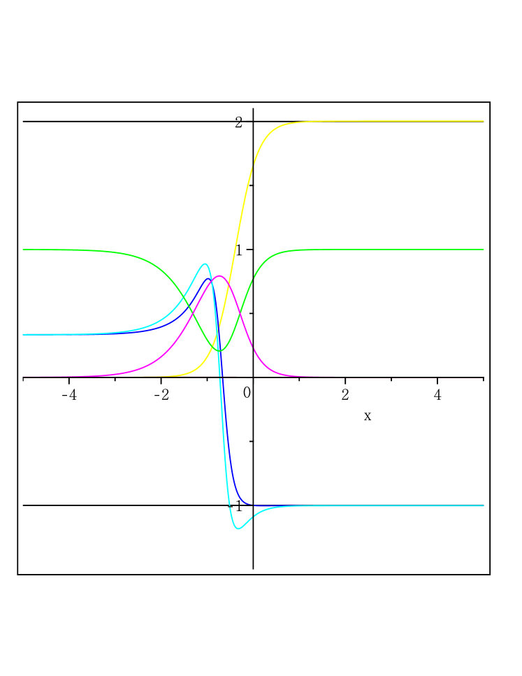
Figure 9: Time evolution of cosmological parameters for exponential case in Jordan frame: $\tilde{w}_{\rm DE}$(blue), $w_{\rm eff}$(cyan), $\Omega_{\rm DE}$(green), $\Omega_{\rm m}$(magenta), $\Omega_{\rm r}$(brown), $r$(yellow), and $F^{\prime}$ (black) for $R_{s}=-0.05,\beta=1.1,\Omega_{\rm m}^{0}=0.23,\chi=3.04\times 10^{-4},h_{1}=-(\frac{3}{2}+\frac{\chi}{2})\Omega_{\rm m}^{0}$.

III.4 Hu and Sawicki case $f(R)=R-\mu R_{c}\left[1-\left(1+\frac{R^{2}}{R_{c}^{2}}\right)^{-n}\right]$

Its derivatives with respect to $R$ are given by

$$F(R) = 1-2\mu n\frac{R}{R_{c}}\left(1+\frac{R^{2}}{R_{c}^{2}}\right)^{-(n+1)},$$ (73)

$$F^{\prime}(R) = -\frac{2\mu n}{R_{c}}\left[1-(2n+1)\frac{R^{2}}{R_{c}^{2}}\right]\left(1+\frac{R^{2}}{R_{c}^{2}}\right)^{-(n+2)}.$$ (74)

Fig. 10 shows that future oscillations around the phantom divide $w_{\rm dS}=-1$ appears for $R_{c}=-1.0,~{}\mu=-1.5,$ and $n=2$ using two equations of state $\tilde{w}_{\rm DE}$ and $w_{\rm eff}$ but there is no evolution toward the past direction from $x_{c}=0$. Also, there are future oscillations around $r_{\rm dS}=2$ for the reduced Ricci scalar $r$. This will be explained in the next section. This confirms the results (Fig. 5) in the Einstein-like frame.

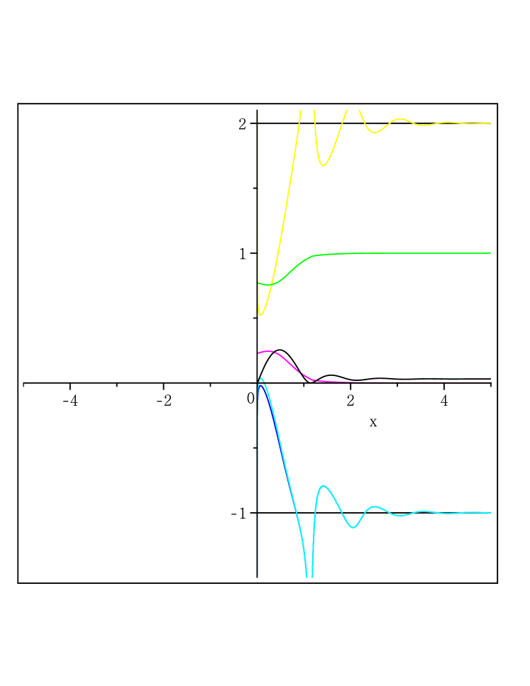
Figure 10: Time evolution of cosmological parameters for Hu and Sawicki case in Jordan frame: $\tilde{w}_{\rm DE}$(blue), $w_{\rm eff}$(cyan), $\Omega_{\rm DE}$(green), $\Omega_{\rm m}$(magenta), $\Omega_{\rm r}$(brown), $r$(yellow), and $F^{\prime}$ (black) for $R_{c}=-1.0,\mu=-1.5,n=2,\Omega_{\rm m}^{0}=0.23,\chi=3.04\times 10^{-4},h_{1}=-(\frac{3}{2}+\frac{\chi}{2})\Omega_{\rm m}^{0}$.

IV Singularity in cosmological evolutions

In this section, we wish to explain the singularities encountered in the cosmological evolution of $f(R)$-fluid Frolov . First of all, we mention that $f(R)$-gravity should satisfy the following bounds: MSY

$$f^{\prime}(R)=F(R)>0,~{}~{}f^{\prime\prime}(R)=F^{\prime}(R)>0.$$ (75)

These are necessary to guarantee that the Newtonian gravity solutions are stable and that the matter-dominated stage remains an attractor with respect to an open set of neighboring cosmological solutions in $f(R)$-gravity. In the perturbation theory, the former is necessary to show that the gravity is attractive and and the graviton is not a ghost, whereas the latter needs to ensure that the scalaron of a massive curvature scalar does not have a tachyon. We show how the singularities appear from the $f(R)$-fluid. From the observation of two equations (18) and (56) which are equivalent to two first Friedmann equations, the second term involves $F^{\prime}(R)$ as the denominator. Hence, if $F^{\prime}(R)=0$ at a certain point of $x=x_{c}$, it gives rise to an singularity at which some cosmological parameters blow up. This results from the violation of stability condition $f(R)$ gravity: the second of (75).

In order to show the presence of singularities explicitly, we use the graph of $F^{\prime}(x)$ as a function of $x$. From Fig. 5, we find that the singularity appears at $x_{c}=0$ and thus, the backward evolution is not allowed in Einstein-like frame. In the Jordan frame, the power-law gravity shows the singularities at $x_{c}\simeq-2.4$ for $\alpha=1/2$ (see Fig. 7) and $x_{c}\simeq-3.4$ for $\alpha=1/3$ (see Fig. 8), while from Fig. 10, we find that the singularity appears at $x_{c}=0$ and thus, the backward evolution is not allowed in Jordan frame. This completes the presence of singularities in the cosmological evolution of $f(R)$-fluid.

V Discussions

We have investigated the issues of future oscillations around the phantom divide for $f(R)$ gravity by introducing two types of energy density and pressure arisen from the $f(R)$-fluid. One has the conventional energy density $\rho_{\rm DE}$ and pressure $p_{\rm DE}$ even in the beginning of the Jordan frame, whose continuity equation provides the native equation of state $w_{\rm DE}=p_{\rm DE}/\rho_{\rm DE}$. Hence, we call this frame as the Einstein-like frame.

On the other hand, the other has the different forms of energy density $\tilde{\rho}_{\rm DE}$ and pressure $\tilde{p}_{\rm DE}$ which do not obviously satisfy the continuity equation. This needs to introduce the effective equation of state $w_{\rm eff}$ to describe the $f(R)$-fluid precisely, in addition to the native equation of state $\tilde{w}_{\rm DE}=\tilde{p}_{\rm DE}/\tilde{\rho}_{\rm DE}$. We confirm that future oscillations around the phantom divide always occur in $f(R)$-gravities by introducing two types of $f(R)$-gravity: one is the power-law potential (33) with the exponent $\alpha=1/2$ and 1/3 and the other is the Hu and Sawiciki model (37). In the Jordan frame, the former did not show past oscillations around the phantom divide and its evolution was terminated around $x_{c}\simeq-2.4$ for $\alpha=1/2$. On the the other hand, the latter did not provide any past evolution in both Einstein-like and Jordan frames. Similarly, we confirm that there are future oscillations around $r_{\rm dS}=2$ for the reduced Ricci scalar $r$ MSY . As was expected, the cosmological constant model has no frame-dependence and we could not find any future oscillations around the phantom divide around $w_{\rm DE}=-1$ for the exponential gravity in (35).

For whole evolution from the past to future when imposing initial conditions at the present time, the cosmological evolution is allowed in the Einstein-like frame better than in the Jordan frame. This means that the cosmological evolution of $f(R)$-fluid determined from its form of energy density and pressure, depending on the given frame. Also, it was proven that the termination (singularity) appeared in cosmological evolution is closely related to the form of $f(R)$-fluid for given frame. This has arisen from $F^{\prime}=0$ in the first Friedmann equations (18) and (56). As a result, it is so because of the violation of the stability condition (non-tachyon) of $f(R)$ gravity.

Consequently, we have successfully performed (whole) cosmological evolution of $f(R)$ gravities by choosing two different state variables of energy density and pressure, and pointed out why the singularity appeared in the backward evolution when the initial condition was chosen as the present time.

- (1) S. Perlmutter et al. [Supernova Cosmology Project Collaboration], Astrophys. J. 517 (1999) 565 [arXiv:astro-ph/9812133]; A. G. Riess et al. [Supernova Search Team Collaboration], Astron. J. 116 (1998) 1009 [arXiv:astro-ph/9805201].
- (2) D. N. Spergel et al. [WMAP Collaboration], Astrophys. J. Suppl. 170 (2007) 377 [arXiv:astro-ph/0603449].
- (3) M. Tegmark et al. [SDSS Collaboration], Phys. Rev. D 69 (2004) 103501 [arXiv:astro-ph/0310723]; D. J. Eisenstein et al. [SDSS Collaboration], Astrophys. J. 633 (2005) 560 [arXiv:astro-ph/0501171].
- (4) B. Jain and A. Taylor, Phys. Rev. Lett. 91 (2003) 141302 [arXiv:astro-ph/0306046].
- (5) S. Nojiri and S. D. Odintsov, eConf C0602061 (2006) 06 [Int. J. Geom. Meth. Mod. Phys. 4, 115 (2007)] [arXiv:hep-th/0601213].
- (6) E. J. Copeland, M. Sami and S. Tsujikawa, Int. J. Mod. Phys. D 15 (2006) 1753 [arXiv:hep-th/0603057].
- (7) T. P. Sotiriou and V. Faraoni, Rev. Mod. Phys. 82, 451 (2010) [arXiv:0805.1726 [gr-qc]].
- (8) S. Nojiri and S. D. Odintsov, arXiv:1011.0544 [gr-qc].
- (9) A. De Felice and S. Tsujikawa, Living Rev. Rel. 13, 3 (2010) [arXiv:1002.4928 [gr-qc]].
- (10) L. Pogosian and A. Silvestri, Phys. Rev. D 77 (2008) 023503 [Erratum-ibid. D 81, 049901 (2010)] [arXiv:0709.0296 [astro-ph]].
- (11) S. Capozziello, M. De Laurentis and V. Faraoni, arXiv:0909.4672 [gr-qc]; K. Nozari and T. Azizi, Phys. Lett. B 680 (2009) 205 [arXiv:0909.0351 [gr-qc]].
- (12) K. Bamba, C. Q. Geng and C. C. Lee, JCAP 1011, 001 (2010) [arXiv:1007.0482 [astro-ph.CO]].
- (13) H. Motohashi, A. A. Starobinsky and J. Yokoyama, JCAP 1106 (2011) 006 [arXiv:1101.0744 [astro-ph.CO]].
- (14) H. W. Lee, K. Y. Kim and Y. S. Myung, Eur. Phys. J. C 71, 1585 (2011) [arXiv:1010.5556 [hep-th]].
- (15) W. Zimdahl and D. Pavon, Phys. Lett. B 521 (2001) 133 [arXiv:astro-ph/0105479].
- (16) V. Paschalidis, S. M. H. Halataei, S. L. Shapiro and I. Sawicki, Class. Quant. Grav. 28 (2011) 085006 [arXiv:1103.0984 [gr-qc]].
- (17) B. Wang, Y. g. Gong and E. Abdalla, Phys. Lett. B 624 (2005) 141 [arXiv:hep-th/0506069].
- (18) H. Kim, H. W. Lee and Y. S. Myung, Phys. Lett. B 632 (2006) 605 [arXiv:gr-qc/0509040].
- (19) K. Y. Kim, H. W. Lee and Y. S. Myung, Mod. Phys. Lett. A 22 (2007) 2631 [arXiv:0706.2444 [gr-qc]].
- (20) K. Bamba, C. Q. Geng and C. C. Lee, JCAP 1008 (2010) 021 [arXiv:1005.4574 [astro-ph.CO]].
- (21) A. V. Frolov, Phys. Rev. Lett. 101 (2008) 061103 [arXiv:0803.2500 [astro-ph]].