Molecular imaging using high-order harmonic generation and above-threshold ionization

Abstract

Accurate molecular imaging via high-order harmonic generation relies on comparing the harmonic emission from a molecule and an adequate reference system. However, an ideal reference atom with the same ionization properties as the molecule does not always exist. We show that for suitably designed, very short laser pulses, a one-to-one mapping between high-order harmonic frequencies and electron momenta in above-threshold ionization exists. Comparing molecular and atomic momentum distributions then provides the electron return amplitude in the molecule for every harmonic frequency. We show that the method retrieves the molecular recombination transition moments highly accurately, even with suboptimal reference atoms.

When atoms or molecules are irradiated by a strong laser field, high-order harmonic generation (HHG) takes place and high-frequency photons are emitted Ferray et al. (1988). The interest in HHG from molecules is growing since observing the radiation is a tool to investigate the structure of molecules Lein et al. (2002a, b); Itatani et al. (2004); Haessler et al. (2010). The sensitivity of the emission spectra to the target structure can be understood within the three-step model, which provides a semiclassical interpretation of HHG in terms of (i) ionization, (ii) free propagation of the electron in the laser field and return to the parent ion, and (iii) recombination Corkum (1993). In good approximation, the HHG intensity is proportional to the modulus squared of the recombination transition dipole moment, or equivalently to the recombination cross section Itatani et al. (2004); van der Zwan et al. (2008); Lin et al. (2010). When the electron continuum states are additionally approximated as plane waves, one can obtain molecular orbitals via a tomographic retrieval based on the Fourier transform of the HHG amplitudes measured from aligned molecules Itatani et al. (2004); Haessler et al. (2010). These HHG-based molecular imaging methods rely on the comparison of the harmonic emission to the one from a reference system with known electronic structure, typically a reference atom. Assuming that the molecule and the reference atom have the same properties concerning ionization probabilities and electron propagation, the recombination cross section of the molecule can be isolated. Clearly, no reference atom with exactly the same ionization properties as the molecule exists. Therefore, a systematic method to correct for these deviations is highly desirable.

Since the probability for recombination of a returning electron is very small, it is likely that the system remains ionized, and the electron can be detected as an above-threshold ionization (ATI) electron. ATI momentum distributions have also be used for molecular imaging Kamta and Bandrauk (2006); Lin et al. (2010); Meckel et al. (2008). It appears plausible to combine HHG and ATI to improve laser-based molecular imaging. For reasons outlined in the following, however, no concrete method has been proposed up to now.

Usually, multi-cycle laser pulses have been used to drive HHG and ATI. This means that many differerent electron trajectories can potentially contribute to the same harmonic frequency or to the same electron momentum. In the case of HHG, the same frequency is generated twice per optical half cycle, namely by the well known short and long trajectory Lewenstein et al. (1994). In the case of ATI, the interference of contributions from two ionization times has been termed attosecond double-slit interference Lindner et al. (2005).

Initially it was thought there would be a direct correspondence between the HHG and ATI spectra (see Toma et al. (1999) and references therein) and attempts were made to express the harmonic yield as a sum over ATI channels plus recombination Kuchiev and Ostrovsky (1999, 2001). However, no direct link between the intensities of individual HHG and ATI peaks could be drawn as in general it is not possible to disentangle the contributions from the different trajectories. Two trajectories producing the same harmonic frequency will generally lead to different ATI energies. Here we show that, for extremely short laser pulses with suitable carrier-envelope phase this link turns out to be possible because only a very limited number of trajectories contributes. Taking also advantage of the exponential dependence of the ionization rate on the field strength, we present strong one-to-one links from HHG frequencies to ATI momenta, based on shared birth times of the HHG and ATI trajectories. We show how to use the relation between HHG and ATI to improve molecular imaging techniques such as orbital tomography.

If there is only one trajectory contributing to each ATI momentum and HHG frequency, and if both trajectories are born at the same time, the ionization steps are identical and there is a one-to-one mapping from HHG frequency $\omega$ to ATI momentum $p^{(\mathrm{A})}(\omega)$. We assume here that the ATI electron is emitted along the laser polarization axis, i.e. there is no rescattering ATI. Then, the HHG intensity $S(\omega)=|\bm{\alpha}(\omega)|2$ and ATI intensity $A(p)=|M(p)|2$ are related by by (atomic units are used throughout) Corkum (1993); van der Zwan et al. (2008); Le et al. (2009)

$$\bm{\alpha}(\omega) =a(\omega)\;\mathbf{v}_{\mathrm{rec}}(\omega),$$ (1a)

$$A(p^{(\mathrm{A})}(\omega)) =C(\omega)\;|a(\omega)|2.$$ (1b)

Here, the complex amplitude $\bm{\alpha}(\omega)$ is the Fourier transformed dipole acceleration and $a(\omega)$ describes the continuum wave packet for HHG. The velocity-form recombination matrix element for the HHG process is denoted $\mathbf{v}_{\mathrm{rec}}(\omega)$. The factor $C(\omega)$ relates HHG and ATI and includes the effect of electron motion after the return time on the momentum distribution. Below, we confirm that $C(\omega)$ only depends on the laser field and is independent of the atom or molecule. This is in contrast to the quantity $a(\omega)$, which is species-dependent. Thus, if the momentum distributions $A(p)$ are known for two different systems, the ratio of their factors $a(\omega)$ can be obtained from Eq. (1b).

Before demonstrating the improved molecular imaging scheme, we find suitable laser pulses for which the one-to-one mapping holds. To this end, we express the HHG and ATI yields using the strong-field approximation and expand around classical trajectories. For HHG we employ the Lewenstein model Lewenstein et al. (1994). In this model, the saddle-point integration over momentum gives the saddle-point momentum $k_{\mathrm{s}}(t,t^{\prime})=-\int_{t^{\prime}}^{t}A(t^{\prime\prime})dt^{\prime\prime}/(t-t^{\prime})$ with $A(t)=-\int_{-\infty}^{t}E(t^{\prime\prime})dt^{\prime\prime}$ such that an electron born at time $t^{\prime}$ returns to its initial position at recombination time $t$. for a linearly polarized laser field $E(t)$. In contrast to Chirilă and Lein (2008); van der Zwan et al. (2008), we perform both remaining integrations over $t^{\prime}$ and $t$ using the saddle-point method. The resulting spectrum is generated by trajectories with complex saddle-point times $t^{\prime}_{\mathrm{s}}$ and $t_{\mathrm{s}}$, starting with imaginary initial momentum $v_{\mathrm{i}}=i\sqrt{2I_{\mathrm{p}}}$ and returning with momentum $v_{\mathrm{r}}=\pm\sqrt{2(\omega-I_{\mathrm{p}})}$ where $I_{\mathrm{p}}$ is the ionization potential. We employ a very short pulse such that all return momenta $v_{\mathrm{r}}$ have the same sign (chosen negative here) van der Zwan and Lein (2008). The classical times $t^{\prime}_{0}$, $t_{0}$ are defined by setting $v_{\mathrm{i}}=0$. We expand the times $t^{\prime}_{\mathrm{s}}$, $t_{\mathrm{s}}$ around $t^{\prime}_{0}$, $t^{\prime}_{0}$ to second order in the Keldysh parameter $\gamma$,

$$t_{\mathrm{s}} =t_{0}+\frac{1}{2}b_{2}\gamma 2;\quad t^{\prime}_{\mathrm{s}}=t^{\prime}_{0}+a_{1}\gamma+\frac{1}{2}a_{2}\gamma 2,$$ (2)

$$a_{1} =\frac{2i\sqrt{U_{\mathrm{p}}}}{|E(t^{\prime}_{0})|};\quad b_{2}=\frac{4U_{\mathrm{p}}}{E(t^{\prime}_{0})(v_{\mathrm{r}}+(t_{0}-t^{\prime}_{0})E(t_{0}))},$$ (3)

$$a_{2} =\frac{4U_{\mathrm{p}}}{(E(t^{\prime}_{0}))2}\left(\frac{E(t_{0})}{v_{\mathrm{r}}+(t_{0}-t^{\prime}_{0})E(t_{0})}+\frac{E^{\prime}(t^{\prime}_{0})}{E(t^{\prime}_{0})}\right).$$ (4)

Expanding to fourth order for the action $S(t,t^{\prime})=\frac{1}{2}\int_{t^{\prime}}^{t}dt^{\prime\prime}\>[k_{\mathrm{s}}(t,t^{\prime})+A(t^{\prime\prime})]2+I_{\mathrm{p}}(t-t^{\prime})$, the resulting expression in a $d$-dimensional world is, denoting the bound state as $\psi_{0}(\mathbf{r})$ and using $\tau_{\mathrm{s}}=t_{\mathrm{s}}-t^{\prime}_{\mathrm{s}}$, $\tau_{0}=t_{0}-t^{\prime}_{0}$,

$$\bm{\alpha}(\omega)= -\omega\left(\frac{I_{\mathrm{p}}}{2}\right)^{-\frac{1}{4}}\mathbf{v}_{\mathrm{rec}}^{*}(v_{\mathrm{r}})\sum_{t_{0},t^{\prime}_{0}}\biggl{[}\frac{2\pi}{\epsilon+i\tau_{\mathrm{s}}}\biggr{]}^{\frac{d}{2}}$$ (5)

$$\times d_{\mathrm{ion}}(-i\>\mathrm{sgn}(E(t^{\prime}_{0}))\sqrt{2I_{\mathrm{p}}},t^{\prime}_{\mathrm{s}})$$

$$\times e^{-i(S(t_{0},t^{\prime}_{0})-\omega t_{0})}e^{if(t_{0},t^{\prime}_{0})\frac{I_{\mathrm{p}}2}{2(E(t^{\prime}_{0}))2}}$$

$$\times\sqrt{{\pi}/{\left(f(t_{0},t^{\prime}_{0})i\sqrt{2I_{\mathrm{p}}}+|E(t^{\prime}_{0})|\right)}}$$

$$\times e^{-\frac{(2I_{\mathrm{p}})^{3/2}}{3|E(t^{\prime}_{0})|}}\sqrt{\frac{2\pi i\tau_{\mathrm{s}}}{{v_{\mathrm{r}}2}+{\tau_{\mathrm{s}}}E(t_{\mathrm{s}})\>v_{\mathrm{r}}}}+\mathcal{O}(\gamma 3),$$

with $f(t_{0},t^{\prime}_{0})=\frac{E(t_{0})}{v_{\mathrm{r}}+\tau_{0}E(t_{0})}+\frac{E^{\prime}(t^{\prime}_{0})}{E(t^{\prime}_{0})}$. The ionization matrix element

$$d_{\mathrm{ion}}(k,t)=\frac{E(t)}{(2\pi)^{d/2}}\int\psi_{0}(\mathbf{r})xe^{-ikx}d^{d}\mathbf{r},$$ (6)

exhibits a pole at the saddle-point momentum for Coulombic potentials. Supported by the fact that HHG can be modeled succesfully using Gaussian bound states that do not exhibit the pole Lewenstein et al. (1994), we replace the integral in Eq. (6) by an arbitrary constant.

Similarly, we expand the ATI amplitude $M(p)$ as given by Milošević et al. Milošević et al. (2002, 2003, 2006) around classical birth times. For detailed derivations of Eqs. (2)–(5) and the analogous ATI expression, see van der Zwan (2010).

We calculate the uniqueness of a trajectory in determining harmonic $\omega$ by dividing the absolute value of the corresponding term in Eq. (5) by the total sum. Similarly, for every harmonic trajectory we also calculate the uniqueness of the ATI trajectory born at the same time in determining its associated ATI momentum. The maximum attainable product of these two factors is labeled $Q(\omega)$. For the maximum possible value $Q=1$, there is a perfect correspondence between a harmonic frequency and ATI momentum through their shared birth time. In Fig. 1(a) we show $Q(\omega)$ for different two-cycle $\sin 2$-laser pulses with intensity $I=2\times 10^{14}$ W/cm² and wavelength $\lambda=2000$ nm shining on a 1D system with the ionization potential set to $I_{\mathrm{p}}=30.2$ eV. The pulses are characterized by the carrier-envelope phase $\phi_{\mathrm{CEP}}$, i.e., the phase between the envelope and the carrier wave of the pulse.

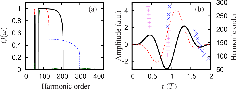
Figure 1: (Color online) (a) $Q(\omega)$ for two-cycle $\sin 2$-pulses with $\phi_{\mathrm{CEP}}=\pi$ (red dashed line), $\phi_{\mathrm{CEP}}=1.25\pi$ (black solid line), $\phi_{\mathrm{CEP}}=1.5\pi$ (blue dotted line) and $\phi_{\mathrm{CEP}}=1.75\pi$ (green dot-dashed line); (b) $E(t)$ (x40, black solid line) and $A(t)$ (red dashed line) for $\phi_{\mathrm{CEP}}=1.25\pi$. Also indicated are the birth (violet plusses) and recombination (blue crosses) times of the dominant trajectories.

We only consider ATI momenta whose amplitudes are greater than $1\,$a.u.

A two-cycle pulse with $\phi_{\mathrm{CEP}}=1.25\pi$ gives rise to a good link between HHG and ATI over a broad harmonic range. This result is nearly independent of the dimensionality $d$ (not shown). In Fig. 1(b) we plot the time-dependent electric field and vector potential of this pulse, and we indicate the birth and recombination times of the dominant trajectories. Because $|E(t)|$ is much higher during the birth time of harmonic orders $\sim 100\text{--}200$ ($t\simeq 0.92T$) than around $t\simeq 1.35T$—the only other time where ATI electrons with the same final momentum are born—the link between HHG and ATI arises. Smartly selecting experimental phase-matching conditions might allow somewhat longer pulses to provide useful links between HHG and ATI. However, for slightly longer pulses the HHG frequencies are linked to very low ATI momenta which may require including Coulomb corrections for the classical trajectories.

We verify the link between HHG and ATI by numerical solution of the time-dependent Schrödinger equation (TDSE) for 1D H${}_{2}^{+}$ with varying internuclear distance $R$. We use the softcore potential

$$V(x)=\frac{-Z}{\sqrt{(x-\frac{R}{2})2+a2}}-\frac{Z}{\sqrt{(x+\frac{R}{2})2+a2}},$$ (7)

where the softness parameter $a2$ is adjusted such that $I_{\mathrm{p}}=30.2$ eV. The TDSE is solved on a grid using the split-operator method Fleck et al. (1976); Feit et al. (1982), and the bound states are found by imaginary-time propagation Kosloff and Tal-Ezer (1986). The grid length is 24027 a.u. and it contains 143360 grid points. After the end of the laser pulse, the wave function is propagated for two more cycles. The HHG spectrum is calculated from a windowed Fourier transform of the dipole acceleration and the ATI spectrum is obtained from the momentum-space representation of the wave function after removing the bound states by windowing out the inner 40 a.u. in position space.

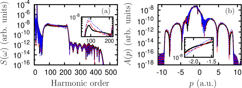
Figure 2: (Color online) (a) HHG spectra for 1D H${}_{2}^{+}$ at $R=2.00$ a.u. (black solid lines), $R=2.03$ a.u. (red dashed lines) and $R=2.06$ a.u. (blue dotted lines). (b) ATI momentum distributions. The insets show smoothed details of the spectra.

For the ground state with $Z=0.731$, the HHG spectra and ATI momentum distributions for three different internuclear distances are shown in Fig. 2. Here we employ the pulse of Fig. 1(b).

Similar to the quantitative rescattering theory Le et al. (2009); Lin et al. (2010), we calculate the 1D recombination matrix elements $v_{\mathrm{rec}}=\langle\psi_{0}(x)|x|\psi_{\mathrm{s}}(x)\rangle$ using field-free scattering states $\psi_{\mathrm{s}}$. We obtain numerically exact $\psi_{\mathrm{s}}$ by integrating the static Schrödinger equation using the Numerov method (see e.g. Blatt (1967)) on a grid with a total length of 4000 a.u. and 320000 grid points. For an electron approaching from positive $x$ we set the wave function equal to $\exp(-ik(\omega)x)$ for the two lowest grid points, where $k(\omega)=\sqrt{2(\omega-I_{\mathrm{p}})}$. After integrating upwards, we require that for large positive $x$ the wave function is given by

$$c\,\psi_{\mathrm{s}}(x)=e^{-ik(\omega)x}+R_{\mathrm{e}}e^{ik(\omega)x},$$ (8)

where $R_{\mathrm{e}}$ is the reflection coefficient. This leads to a normalization constant

$$c=2e^{-ik(\omega)x}/\left(\psi_{\mathrm{s}}(x)+i\psi_{\mathrm{s}}^{\prime}(x)/k\right).$$ (9)

In Fig. 3 we demonstrate the link between HHG and ATI as a function of $R$ using the other parameters of Fig. 2.

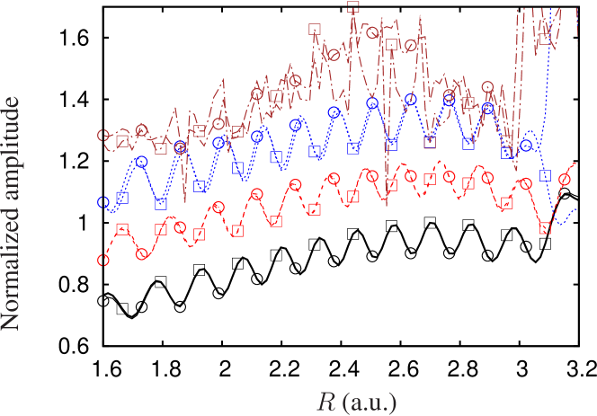
Figure 3: (Color online) Vertically aligned $|a(\omega)|$ (lines with circles) and $\sqrt{A(p^{(\mathrm{A})}(\omega))}$ (lines with squares) as a function of $R$. We consider harmonic orders 100 (black solid lines), 150 (red dashed lines), and 200 (blue dotted lines) and their associated ATI momenta $p^{(\mathrm{A})}=-1.4922$ a.u., $p^{(\mathrm{A})}=-1.8301$ a.u., and $p^{(\mathrm{A})}=-2.2315$ a.u., respectively. The curves were shifted vertically for clarity. Also shown are harmonic 150 and ATI momentum $p^{(\mathrm{A})}=-1.8301$ a.u. from a six-cycle trapezoidal pulse with 1-cycle ramps (brown dot-dashed lines), for comparison.

For three different harmonic orders we plot $|a(\omega)|$ and $\sqrt{A(p^{(\mathrm{A})}(\omega))}$ (both normalized) using the links between HHG and ATI obtained from Eqs. (5) and the corresponding ATI expression. The remarkable overlap between HHG and ATI that only breaks down for the largest $R$ confirms the strong link between HHG and ATI indicated by the black solid line in Fig. 1(a). The ratios of normalization constants correspond to $\sqrt{C(\omega)}$ (see Eq. (1b)). The oscillation in $R$ of both the HHG and ATI amplitudes in Fig. 3 is caused by excitation to the first excited state before ionization. Between two maxima the first excited state drops in energy by exactly $\omega$. We have verified that the oscillation period is inversely proportional to the laser wavelength prior to the moment of ionization. Both the fact that the HHG and ATI curves for a six-cycle pulse are less similar to each other and the fact that they exhibit wild behavior are related to multiple trajectories contributing to the yields.

The link between HHG and ATI gives the experimentalist access to the ratio of the instanteneous ionization rates of different molecules during the high-harmonic generation process, and as such is a useful tool in studying HHG and molecular imaging. In particular, the estimate for the continuum wave packet needed for the tomographic reconstruction of molecular orbitals Itatani et al. (2004) can be improved using

$$a_{\theta}(\omega)=a^{(a)}(\omega)\sqrt{A_{\theta}(p^{(\mathrm{A})}(\omega))/A^{(a)}(p^{(\mathrm{A})}(\omega))}.$$ (10)

Here $\theta$ is the orientation of the molecule in the laser field and with the superscript ‘$(a)$’ we denote quantities belonging to the reference atom in the tomographic procedure. Demonstrating numerically the possibility of combined HHG-ATI molecular imaging, we retrieve the field-free matrix elements of the first excited state of 1D H${}_{2}^{+}$ using a reference atom. We employ

$$v_{\mathrm{rec}}(\omega)\simeq\alpha(\omega)/a(\omega)$$ (11)

with either $a(\omega)=a^{(a)}(\omega)P_{\mathrm{I}}/P_{\mathrm{I}}^{(a)}$ (HHG imaging), where $P_{\mathrm{I}}$ is the total ionization probability, or with Eq. (10) (HHG-ATI imaging). Here we use for 1D H${}_{2}^{+}$ the parameters $R=2$ and $Z=1.3$ a.u. and the same laser pulse as for Fig. 2. As the reference atom we use 1D softcore models with different nuclear charges $Z^{(a)}$. For all systems the softcore parameter $a2$ is adjusted such that $I_{\mathrm{p}}=30.2$ eV. The results of the simulation can be found in Fig. 4.

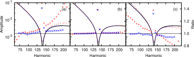
Figure 4: (Color online) Exact matrix element $v_{\mathrm{rec}}(\omega)$ for the first excited state of H${}_{2}^{+}$ (black solid lines), recovered matrix element using only HHG (red dashed lines) and recovered matrix elements using HHG and ATI (blue dotted lines). Also shown is the ratio of the recovered to the exact matrix elements on a linear scale using only HHG (red plusses) and using HHG and ATI (blue crosses); (a) $Z^{(a)}=1.4$ a.u., (b) $Z^{(a)}=2.6$ a.u., (c) $Z^{(a)}=4$ a.u.

The figure shows that when the total nuclear charge is identical for the molecule and the reference atom (Fig. 4(b)), the molecular matrix element can be accurately retrieved using only HHG from the molecule and atom Zeidler et al. (2006), thereby also demonstrating the accurateness of our field-free matrix elements Lin et al. (2010). However, when the total nuclear charge does not match (Figs. 4(a) and 4(c)) the propagation step becomes different for the atom and molecule and errors arise in the retrieval of the matrix elements. These errors largely disappear by incorporating also ATI electrons in the retrieval procedure, demonstrating the potential of Eq. (10) for orbital tomography and molecular imaging in general. The shallowing of the retrieved matrix elements comes from diffusing the HHG and ATI spectra with Gaussians with $1/e$-widths of $\Delta\omega=6\omega_{\mathrm{L}}$ a.u. and $\Delta p=2\sqrt{0.2\omega_{\mathrm{L}}}$ a.u., respectively.

In summary, we used the saddle-point approximation and expansions in $\gamma$ to evaluate strong-field expressions for HHG and ATI in terms of sums over classical trajectories. Using these expressions we have shown that for extremely short laser pulses and long laser wavelengths there exists strong links between individual frequencies and momenta of HHG and ATI. We demonstrated these links and their potential for molecular imaging using 1D model calculations. Future molecular imaging experiments will benefit from this effect.