The Similarity Renormalization Group with Novel Generators

Abstract

The choice of generator in the Similarity Renormalization Group (SRG) flow equation determines the evolution pattern of the Hamiltonian. The kinetic energy has been used in the generator for most prior applications to nuclear interactions, and other options have been largely unexplored. Here we show how variations of this standard choice can allow the evolution to proceed more efficiently without losing its advantages.

I Introduction

The Similarity Renormalization Group (SRG) uses a continuous series of unitary transformations to decouple high-momentum and low-momentum physics in an input Hamiltonian Glazek and Wilson (1993); Wegner (1994). This decoupling means that expansions of physical observables generally become more convergent. The SRG can be implemented through a flow equation for the evolving Hamiltonian $H_{s}$,

$$\frac{dH_{s}}{ds}=[\eta_{s},H_{s}]=[[G_{s},H_{s}],H_{s}]\;,$$ (1)

where $s$ is a flow parameter Wegner (1994); Kehrein (2006) and the generator $\eta_{s}$ is specified by the operator $G_{s}$. With $G_{s}$ chosen to be the relative kinetic energy $T_{\rm rel}$, the SRG has been applied successfully over the past few years to calculate nuclear structure and reactions Bogner et al. (2007a, 2008); Jurgenson et al. (2009); Hebeler et al. (2011); Bogner et al. (2010); Navratil et al. (2010, ); Jurgenson et al. (2011); Hergert et al. (2011). However, different choices for $G_{s}$ will give rise to different patterns of evolution, which may be advantageous. In this paper, two alternatives to $T_{\rm rel}$ are evaluated for their effectiveness in decoupling and, in particular, for improvements in computing speed (see Fig. 1 for a representative example). Our tests are for realistic nucleon-nucleon (NN) interactions in two-body systems and for a one-dimensional model Hamiltonian applied to few-body bound states.

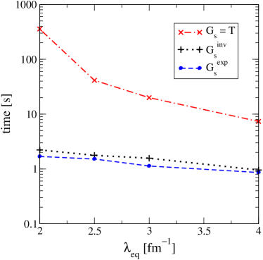
Figure 1: (Color online) Computational time to evolve the Argonne $v_{18}$ ¹S₀ potential Wiringa et al. (1995) as a function of the final value of $\lambda_{\rm eq}$ (see text) for several generators, with $\sigma=2\,\,\text{fm}^{-1}$ for $G_{s}^{\rm inv}$ and $G_{s}^{\rm exp}$.

We focus on novel generators that have $G_{s}$ as functions of $T_{\rm rel}$. (Note: we can just as well consider the full kinetic energy $T$ in our discussion, because the center-of-mass part commutes with the running Hamiltonian $H_{s}$, so we will use $T$ for convenience.) In particular, we explore the “inverse” $G_{s}$ operator

$$G_{s}=-\frac{\sigma^{2}}{1+T/\sigma^{2}}\equiv G_{s}^{\rm inv}\;,$$ (2)

and the “exponential” $G_{s}$ given by

$$G_{s}=-\sigma^{2}e^{-T/\sigma^{2}}\equiv G_{s}^{\rm exp}\;.$$ (3)

Each has a Taylor series that reduces to $T$ (up to a constant, which drops out from the commutator) at low momentum or when $\sigma$ is large. As such, the independent parameter $\sigma$ controls the separation of a low-energy region where $G_{s}$ behaves as $T$ and the potential is driven toward the diagonal, and a high-energy region where evolution is suppressed. This suppression can result in a significant computational speedup of the SRG evolution when compared to calculations with $G_{s}=T$, while not impacting the advantageous properties of the evolution for low-momentum applications.

The generators’ suppression of running in unneeded parts of the Hamiltonian could mitigate the difficulties of evolving very large matrices for calculations of light atomic nuclei Jurgenson et al. (2011), opening the door to more tailored SRG generators and more effective evolution of three- and eventually four-body interactions. Even at the two-body level there are problems when trying to evolve to large values of the flow parameter $s$. A recent example is a study of SRG decoupling with large-cutoff effective field theory (EFT) potentials, which require evolution beyond the range usually considered Wendt et al. (2011). In doing so, the SRG differential equations can become extremely stiff and take a prohibitively long time (weeks on a single processor) to evolve. This problem has hindered exploratory studies into issues such as what happens when a chiral EFT is evolved to the regime of pionless EFT.

In Sec. II, we give representative results for applications to two-body systems, including an analysis of the flow pattern. These results are extended to few-body systems in Sec. III using a model one-dimensional Hamiltonian that has proved useful in past applications Jurgenson and Furnstahl (2009); Anderson et al. (2010). We summarize and outline future studies in Sec. IV.

II Two-nucleon systems

In this section we give representative results for evolving realistic nucleon-nucleon potentials using the novel generators from Eqs. (2) and (3) in comparison to the usual choice of $G_{s}=T$.

II.1 Performance

The key advantage of the generators that we highlight is the improvement in computational performance. For example, the time needed to evolve the Argonne $v_{18}$ ¹S₀ potential Wiringa et al. (1995) to equivalent levels of decoupling with several generators is plotted in Fig. 1. The parameter $\lambda\equiv 1/s^{1/4}$, which has dimensions of a momentum, has been used to identify the momentum decoupling scale. However, different generators will evolve a given potential at different rates, so comparing results with the same definition of $\lambda$ can be misleading. Therefore, we identify an “equivalent” $\lambda_{\rm eq}$ for each generator that equalizes the degree of decoupling compared to $G_{s}=T$ (for which $\lambda_{\rm eq}=\lambda$ by definition); the details are described in Sec. II.2.

The value of $\sigma$ will also have an impact, as discussed below; in Fig. 1 we use the intermediate value $\sigma=2\,\text{fm}^{-1}$. With this choice, there is nearly an order of magnitude difference in the time to evolve the Argonne $v_{18}$ potential with $G_{s}^{\rm exp}$ and $G_{s}^{\rm inv}$ compared to $G_{s}=T$ at $\lambda_{\rm eq}=4\,\text{fm}^{-1}$ and two orders of magnitude by $\lambda_{\rm eq}=2\,\text{fm}^{-1}$. Note that nuclear interactions typically have been evolved for nuclear structure studies in the range $\lambda=1.5$–$2.2\,\text{fm}^{-1}$. The speed gains will depend on the initial potential and can be much less for the evolution of softer initial potentials; e.g., for the N³LO 500 MeV chiral EFT potential of Ref. Entem and Machleidt (2003), evolving with $G_{s}^{\rm exp}$ to $\lambda_{\rm eq}=2\,\text{fm}^{-1}$ is about 1.5 times as fast as with $G_{s}=T$ and about 3 times as fast to $\lambda_{\rm eq}=1.5\,\text{fm}^{-1}$.

The numerical solution of the SRG evolution equations requires repeated dense matrix-matrix multiplications. As a consequence, the evolution has been carried out on shared-memory computer architectures. Recent calculations using the SRG with many-body forces are approaching the limits of what is practical to evolve in memory on a single node because of the size of the model space needed Jurgenson et al. (2011). A distributed scheme to solve the equations would permit larger model spaces to be utilized; however, the dense matrix multiplication would then be limited by internode communication times. The reduced number of operations required by novel generators might help make such a scheme possible.

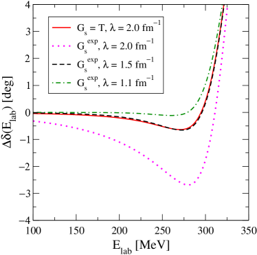
Figure 2: (Color online) Deviation of phase shifts calculated with the Argonne $v_{18}$ ¹S₀ potential Wiringa et al. (1995) evolved with $G_{s}=T$ and $G_{s}^{\rm exp}$ ($\sigma=2\,\,\text{fm}^{-1}$) to various $\lambda$ values and then truncated at $k_{\rm cut}=2\,\,\text{fm}^{-1}$ to test decoupling. Phase shifts from untruncated potentials agree precisely with those from the initial potential.

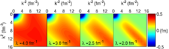
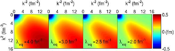
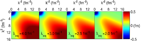
Figure 3: (Color online) Contour plots showing the evolution via Eq. (1) at several values of $\lambda_{\rm eq}$ starting from the momentum-space Argonne $v_{18}$ ¹S₀ potential Wiringa et al. (1995) using (a) $G_{s}=T$, (b) $G_{s}^{\rm inv}$ from Eq. (2) with $\sigma=2\,\,\text{fm}^{-1}$, and (c) $G_{s}^{\rm exp}$ from Eq. (3) with $\sigma=2\,\,\text{fm}^{-1}$.

II.2 Decoupling and $\lambda_{\rm eq}$

To validate the apparent computational advantages of these generators, one must confirm that the decoupling characteristics of the $G_{s}=T$ generator are also reproduced, so that calculations of physical observables also become more convergent. However, if we evolve to the same $\lambda$, the degree of decoupling for identical initial potentials differs for $G_{s}^{\rm exp}$ and $G_{s}^{\rm inv}$ compared to $G_{s}=T$. These differences are evident in the deviations of ¹S₀ phase shifts calculated from the evolved potentials using $G_{s}^{\rm exp}$ and $G_{s}=T$ from the unevolved potential shown in Fig. 2 for several different $\lambda$ values (only $G_{s}^{\rm exp}$ is shown; $G_{s}^{\rm inv}$ behaves similarly). If the full potentials were used, the phase shifts would agree – up to numerical precision – with those from the initial potential, because the evolution in all cases is unitary. However, the degree of decoupling for a given value of $\lambda$ can be made manifest by first cutting off the potential (that is, setting its matrix elements to zero) above some value of $k$ and then calculating the phase shifts. In Fig. 2, for illustration, we choose the cutoff value $k_{\rm cut}$ to be $2\,\text{fm}^{-1}$. The signature of decoupling is that the phase shifts agree at lower energies and only deviate close to and above the cutoff. This is typically observed when the potential is evolved so that $\lambda$ is less than the cut momentum Jurgenson et al. (2008); Bogner et al. (2007b).

This behavior provides us with a pragmatic way to define $\lambda_{\rm eq}$: identifying it with the decoupling behavior that is found for $G_{s}=T$ for a given $\lambda$. We use the results in Fig. 2 to illustrate the procedure. The continuous curve shows the deviation of phase shifts for the potential evolved with $G_{s}=T$ to $\lambda=2\,\,\text{fm}^{-1}$ and cut at $k=2\,\,\text{fm}^{-1}$. As expected from decoupling, the deviation is small up to roughly $k_{\rm cut}$. We use this level of agreement as the criterion for identifying equivalent $\lambda$’s for other generators. That is, a potential is evolved to a series of $\lambda$ values with a different $G_{s}$ and then cut at $k_{\rm cut}$ after evolution. The phase shifts are then compared to the level of decoupling observed for $G_{s}=T$ at $k_{\rm cut}=\lambda$. The approximate point in the novel $G_{s}$ evolution for which the cut phase shifts agree is equated with $\lambda_{\rm eq}$. Consider the phase shifts for the potential evolved with $G_{s}^{\rm exp}$ to several values of $\lambda$ and cut at $k=2\,\,\text{fm}^{-1}$, as shown in Fig. 2. For $G_{s}^{\rm exp}$, $\lambda$ evolved to $1.5\,\,\text{fm}^{-1}$ gives a similar degree of decoupling as $\lambda$ evolved to $2\,\,\text{fm}^{-1}$ with $G_{s}=T$. As a result, we define $\lambda=1.5\,\,\text{fm}^{-1}$ to be the $\lambda_{\rm eq}=2\,\,\text{fm}^{-1}$ for $G_{s}^{\rm exp}$. We use $\lambda_{\rm eq}$ for most comparisons in the following discussion.

II.3 Flow Analysis

Having chosen a working definition for the decoupling scale of evolution with our novel generators, we take a closer look at the properties of the evolved potentials. In particular, we would like to see how a potential flows with evolution using these generators compared to $G_{s}=T$ and to understand how the choice of $\sigma$ affects this flow.

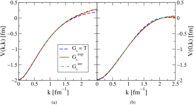
Figure 4: (Color online) Diagonal (a) and off-diagonal (b) momentum-space matrix elements for evolved Argonne $v_{18}$ ¹S₀ potential Wiringa et al. (1995) with $G_{s}=T$ and generators $G_{s}^{\rm exp}$ and $G_{s}^{\rm inv}$ at $\lambda=2\,\text{fm}^{-1}$ with $\sigma=2\,\,\text{fm}^{-1}.$

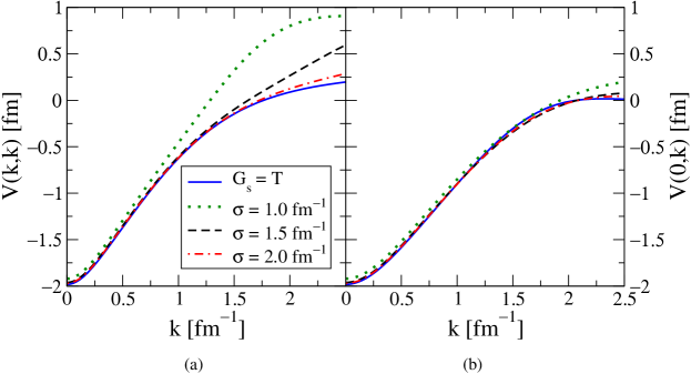
Figure 5: (Color online) Diagonal (a) and off-diagonal (b) momentum-space matrix elements for evolved Argonne $v_{18}$ ¹S₀ potential Wiringa et al. (1995) with $G_{s}=T$ and $G_{s}^{\rm exp}$ with different values of $\sigma$ each evolved to $\lambda=2\,\text{fm}^{-1}$. The lines with $\sigma=3\,\,\text{fm}^{-1}$ are indistinguishable from the ones with $G_{s}=T$.

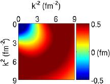
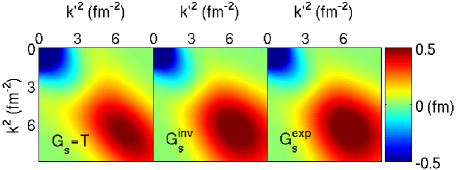
Figure 6: (Color online) (a) Unevolved N³LO 500 MeV ¹S₀ potential . (b) Contour plot showing the evolved N³LO ¹S₀ potential with different generators to $\lambda_{\rm eq}=2\,\text{fm}^{-1}$. For $G_{s}^{\rm exp}$ and $G_{s}^{\rm inv}$, $\sigma=2\,\text{fm}^{-1}.$

In Fig. 3 we compare the evolution pattern of the two-body potential in the ¹S₀ channel with different generators. Each frame is a representation of the potential matrices in momentum space; where the matrix is zero, there is no coupling between momentum components. The initial potential in all cases is Argonne $v_{18}$ Wiringa et al. (1995) and the value of $\sigma$ is taken to be $2\,\,\text{fm}^{-1}$. Note that at $\lambda=4\,\text{fm}^{-1}$, the first matrix plotted here, there is already significant evolution. As the potential is evolved, its high and low momentum components become increasingly decoupled, as expected. It is evident that the evolved potentials are similar (but not identical) in the region where $k^{2},k^{\prime}{}^{2}<\sigma^{2}$. When $\lambda<\sigma$ we find that $\sigma$ roughly defines the low-momentum region where these generators behave as $G_{s}=T$. The minor differences in this low-momentum region can be attributed to the fact that the point in evolution, $\lambda$, needed for these generators to reach the corresponding $\lambda_{\rm eq}$ occurs when $\lambda<\lambda_{\rm eq}$. At higher momenta, novel generator evolution is suppressed relative to $G_{s}=T$. The patterns here are characteristic of the particular generator and are similar for other potentials and in other channels.

This nature of the evolution is further illustrated by the plots in Figs. 4 and 5, which show a detailed view of the diagonal and off-diagonal values of the matrices at low momentum for each generator applied to the Argonne $v_{18}$ ¹S₀ potential . The flow parameter was run to $\lambda=2\,\text{fm}^{-1}$ with the generators here to distinguish between ambiguities caused by using $\lambda_{\rm eq}$. In Fig. 4, the values from different generators agree quite well for $k<\sigma$, where $\sigma\approx\lambda$. Moreover, we see that the minor “pincushion” effect seen in Fig. 3 for these generators relative to $G_{s}=T$ is indeed an artifact of using $\lambda_{\rm eq}$, as each curve falls to zero at approximately the same time. In Fig. 5 we focus on $G_{s}^{\rm exp}$ versus $G_{s}=T$ and the fact that they differ for $\sigma\leq\lambda$. However, as $\sigma\rightarrow\lambda$ it is evident that the evolution of the novel generator becomes increasingly similar to $G_{s}=T$ in the low-momentum region $k<\lambda$. For larger values of $\sigma,$ these generators become indistinguishable from $G_{s}=T$.

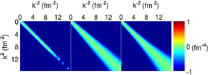
Figure 7: (Color online) Color contour plots of the first term (excluding the factor due to $V_{s}$) on the right side of Eq. (6) for $G_{s}=T$ (left), $G_{s}^{\rm inv}$ (middle), and $G_{s}^{\rm exp}$ (right). The last two use $\sigma=2\,\text{fm}^{-1}$.

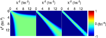
Figure 8: (Color online) Color contour plots of the first terms (excluding the factor due to $V_{s}$) on the right side of Eq. (6) for $G_{s}^{\rm exp}$ with $\sigma=1,2,$ and $3\,\text{fm}^{-1}$ from left to right.

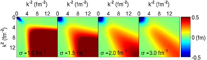
Figure 9: (Color online) Contour plot showing the evolution to $\lambda_{\rm eq}=2\,\text{fm}^{-1}$ via Eq. (1) starting from the momentum-space Argonne $v_{18}$ ¹S₀ potential Wiringa et al. (1995) using $G_{s}^{\rm exp}$ from Eq. (3) with different values of $\sigma$.

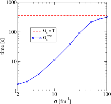
Figure 10: (Color online) Computational time to evolve the Argonne $v_{18}$ ¹S₀ potential Wiringa et al. (1995) with $G_{s}=T$ and $G_{s}^{\rm exp}$ to $\lambda_{\rm eq}=2\,\text{fm}^{-1}$ as a function of the value of $\sigma$.

As a demonstration of similar behavior for different NN potentials, an evolved potential with different generators in the ¹S₀ channel of the N³LO 500 MeV potential Entem and Machleidt (2003) is shown in Fig. 6. Note that the initial potential has significantly less coupling at high momentum compared to Argonne $v_{18}$ Bogner et al. (2010). As a result, there is correspondingly less improvement in evolution speed. However, the general features of the evolution patterns with different generators seen with Argonne $v_{18}$ are also seen for the N³LO potential.

To better understand the evolution process, we need to look further into the flow equation itself. Evaluating Eq. (1) in a two-body partial-wave momentum space basis with $G_{s}=T$ yields

$$\frac{dV_{s}(k,k^{\prime})}{ds} = -(k^{2}-k^{\prime}{}^{2})^{2}V_{s}(k,k^{\prime})$$ (4)

$$\hbox{}+\frac{2}{\pi}\int_{0}^{\infty}q^{2}dq\,(k^{2}+k^{\prime}{}^{2}-2q^{2})V_{s}(k,q)V_{s}(q,k^{\prime})\;.$$

In the far off-diagonal region, the first term dominates (this is true for the ordinary range of $\lambda$ but is modified when $\lambda$ is comparable with the binding momentum of a bound state). This implies that each off-diagonal matrix element is driven to zero as

$$V_{s}(k,k^{\prime})\stackrel{{\scriptstyle k\neq k^{\prime}}}{{\longrightarrow}}V_{s=0}(k,k^{\prime})\,e^{-s(k^{2}-k^{\prime}{}^{2})^{2}}\;.$$ (5)

For $G_{s}=f(T)$, these results are modified to

$$\frac{dV_{s}(k,k^{\prime})}{ds} = -\bigl{(}k^{2}-k^{\prime}{}^{2}\bigr{)}\bigl{(}f(k^{2})-f(k^{\prime}{}^{2})\bigr{)}V_{s}(k,k^{\prime})$$ (6)

$$\hbox{}+\frac{2}{\pi}\int_{0}^{\infty}q^{2}dq\,\bigl{(}f(k^{2})+f(k^{\prime}{}^{2})-2f(q^{2})\bigr{)}$$

$$\hbox{}\hbox{}\times V_{s}(k,q)V_{s}(q,k^{\prime})\;$$

and

$$V_{s}(k,k^{\prime})\stackrel{{\scriptstyle k\neq k^{\prime}}}{{\longrightarrow}}V_{s=0}(k,k^{\prime})\,e^{-s(k^{2}-k^{\prime}{}^{2})(f(k^{2})-f(k^{\prime}{}^{2}))}\;.$$ (7)

The difference in the exponents of Eqs. (5) and (7) for $k\sim\lambda$ leads to $\lambda_{\rm eq}<\lambda$.

The first term of the flow equation (excluding the factor due to the potential) for each of our generators is shown as a contour plot in Figs. 7 and 8. In Fig. 7 we see that $T$ works uniformly (in $k^{2}$) on the entire region of the potential. With $G_{s}^{\rm inv}$, there is much less evolution close to the diagonal. The plot for $G_{s}^{\rm exp}$ is similar, but exhibits even less evolution in the middle region.

It is evident here that the novel generators will result in less evolution at high momenta, as we have seen, and that this should be a generic result for other partial waves and for higher-body evolution, because it depends on only kinetic energy differences. We also see how the value of $\sigma$ controls the degree to which the operator $G_{s}$ is similar to $T$. This is illustrated in Fig. 8. If $\sigma=1\,\,\text{fm}^{-1}$, only the edges of the potential are modified; the shape is completely different from $T$. For $\sigma=3\,\,\text{fm}^{-1}$, there is the thinnest band on the diagonal, which is closest to $T$. At very large $\sigma$, there is a transition to $T$. In the plots of Fig. 9 we see how the final evolved flow is affected by differing choices of $\sigma$.

The limited evolution at high momenta seen in these generators suggests that the time to evolve to a given decoupling parameter $\lambda_{\rm eq}$ should be less for $G_{s}^{\rm inv}$ or $G_{s}^{\rm exp}$ than for $G_{s}=T$. The dramatic drop in evolution time seen in Fig. 1 for the generators makes it apparent that they are more efficient. However, we can also look at how the choice of $\sigma$ affects their performance. This is shown in Fig. 10 for $G^{\rm exp}_{s}$, where we see that the time spent evolving to $\lambda_{\rm eq}=2\,\,\text{fm}^{-1}$ decreases as $\sigma$ decreases. As $\sigma$ becomes smaller, the evolution at high momentum is increasingly limited, which we correlate with improvement in computation time; as $\sigma$ increases, the evolution time approaches that of $T$ (as does the flow). Note that for the Argonne $v_{18}$ potential a large $\sigma$ is needed before $G_{s}$ is effectively equal to $T$.

In practical applications, one might optimize the trade-off between decoupling and computational speedup by choosing $\sigma$ to be approximately equal to, or slightly greater than the $\lambda$ corresponding to $\lambda_{\rm eq}$. Then the decoupling properties of $G_{s}=T$ are preserved in the low momentum region of interest while still enhancing the computational performance of the evolution by limiting the evolution at high momentum. However, this prescription has not yet been tested in detail.

III Few-body tests in a one-dimensional model

The effects on matrices in a momentum basis demonstrated in the last section are generic and so should carry over to alternative bases and to higher-body forces. Calculations for realistic three-dimensional few-body systems are not yet available, but we can test the generators in a one-dimensional model of bosons that has proven to accurately predict the evolution of three-dimensional few-body forces Jurgenson and Furnstahl (2009). The model we use was originally introduced in Ref. Alexandrou et al. (1989) as a sum of two Gaussians to simulate repulsive short-range and attractive mid-range nucleon-nucleon two-body potentials. It is written in coordinate space as

$$V^{(2)}(x)=\frac{V_{1}}{\sigma_{1}\sqrt{\pi}}e^{-x^{2}/\sigma_{1}^{2}}+\frac{V_{2}}{\sigma_{2}\sqrt{\pi}}e^{-x^{2}/\sigma_{2}^{2}}$$ (8)

and in momentum space as

$$V^{(2)}(p,p^{\prime})=\frac{V_{1}}{2\pi\sqrt{2}}e^{-(p-p^{\prime})^{2}\sigma_{1}^{2}/8}+\frac{V_{2}}{2\pi\sqrt{2}}e^{-(p-p^{\prime})^{2}\sigma_{2}^{2}/8}\;,$$ (9)

where $V_{1}=12$, $\sigma_{1}=0.2$, $V_{2}=-12$, and $\sigma_{2}=0.8$ (see Ref. Alexandrou et al. (1989) for discussion of units). Also, in calculations with an initial three-body potential, a regulated contact interaction is used. This is written as

$$V^{(3)}(p,q,p^{\prime},q^{\prime})=c_{E}\,f_{\Lambda}(p,q)f_{\Lambda}(p^{\prime},q^{\prime}),$$ (10)

where $c_{E}$ corresponds to the strength of the interaction and

$$f_{\Lambda}(p,q)=e^{-((p^{2}+q^{2})/\Lambda^{2})^{n}}.$$ (11)

The regulator cutoff $\Lambda=2$, and the sharpness of the fall off is set to $n=4$. We have chosen these parameters for comparison with Ref. Jurgenson and Furnstahl (2009).

III.1 Performance

Basis	Momentum	Oscillator
System	$A=2$	$A=2$	$A=3$	$A=4$
$\sigma=2$	3.3	3.3	3.8	4.1
$\sigma=3$	2.6	2.6	2.7	2.8

Table 1: Speed up in model $A$-particle one-dimensional (1D) oscillator basis for evolution to $\lambda_{eq}\approx 3$, comparing the ratio of the time to evolve $G_{s}=T$ versus $G_{s}^{\rm exp}$. The results for $G_{s}^{\rm inv}$ are very similar.

Our first test is to confirm that the enhanced computational performance characteristics of these generators are maintained in the few-body basis. Table 1 shows the speedup obtained using the $G_{s}^{\rm exp}$ generator with the model potential described previously. The performance of the $G_{s}^{\rm inv}$ generator is very similar to the $G_{s}^{\rm exp}$ results quoted here. Results are reported at an optimal $\lambda_{\rm eq}$; we do not use a range of $\lambda$ values here because of the particularities of the oscillator basis convergence properties, which is discussed in more detail in what follows.

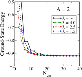
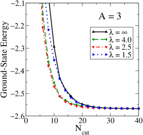
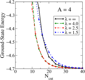
Figure 11: (Color online) Decoupling using $G_{s}^{\rm exp}$ with $\sigma=3$ for (a) $A=2$, (b) $A=3$, and (c) $A=4$. The initial two-body-only potential is evolved to each $\lambda$ shown in a basis with $N_{\rm max}=40$. Matrix elements of the potential are set to zero if one or both states have $N>N_{\rm cut}$ and the resulting Hamiltonian is diagonalized to obtain the ground-state energies plotted.

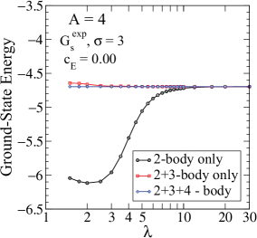
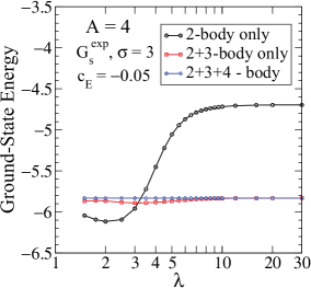
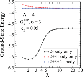
Figure 12: (Color online) The lowest bound-state energy for a four-particle system as a function of $\lambda$ evolved using the SRG $G_{s}^{\rm exp}$ generator and an $N_{\rm max}=40$ basis with an initial three-body potential with strength (a) $c_{\rm E}=0.0$, (b) $c_{\rm E}=-0.05$, and (c) $c_{\rm E}=0.05$. The (blue) curves with diamonds include the full evolution of the Hamiltonian while the (black) curves with circles use the two-body potential evolved in the two-particle system and the (red) curves with squares use the two- and three-body potentials evolved in the three-particle system. Evolution with $G_{s}^{\rm inv}$ is almost indistinguishable.

We find that the evolution of the two-body force in two-, three-, and four-particle systems with novel generators are all 2.5–4 times faster than the evolution with $G_{s}=T$ (to the same degree of decoupling). The performance enhancement is relatively basis independent, with the speedup for the momentum and oscillator bases roughly equivalent. While the speedup improvement is much smaller than that found for Argonne $v_{18}$, we do not expect a direct correspondence. The important point is that the speedup in the A=2 particle system serves as a good predictor of the speedup in the A=3 and A=4 systems. Thus, one might expect a similar improvement in few-body oscillator basis calculations with Argonne $v_{18}$ as found previously for Argonne $v_{18}$ in the two-particle partial-wave momentum basis. This will be significant as we move to novel generator calculations in realistic three-dimensional systems.

III.2 Decoupling

The measure of performance using these generators depends explicitly on their decoupling properties in the few-body harmonic oscillator basis relative to $G_{s}=T$. Ultimately, we find the level of decoupling obtained with $G_{s}=T$ to be matched by these generators.

However, the convergence properties of the oscillator basis with respect to SRG evolution, and consequently the issue of selecting an appropriate $\lambda_{\rm eq}$ in this basis, is more complicated than for the momentum basis. The convergence of observables depends on a balance of the ultraviolet (UV) and infrared (IR) cutoffs intrinsic to the choice of a particular oscillator basis. These cutoffs are given by Jurgenson et al. (2011)

$$\Lambda_{\rm UV}\sim\sqrt{mN_{\rm max}\hbar\Omega}$$ (12)

and

$$\Lambda_{\rm IR}\sim\sqrt{\frac{m\hbar\Omega}{N_{\rm max}}}\;,$$ (13)

where $\Omega$ is the oscillator frequency and $N_{\rm max}$ is the maximum number of total oscillator excitations in the basis. Thus, a cutoff in oscillator basis states results in two approximate cutoffs in momentum space. However, the SRG, using the generators considered here, provides only a means to effectively lower the UV cutoff (by decoupling high- and low-momentum degrees of freedom in the Hamiltonian). As such, convergence is not monotonically improved with respect to evolution in $\lambda$.

As a measure of the decoupling, we plot the binding energy of the lowest energy state for an $A$-particle system with respect to $N_{\rm cut}$ for evolutions of the initial Hamiltonian to various $\lambda$ (this procedure was carried out for $G_{s}=T$ using this model in Jurgenson and Furnstahl (2009)). The actual calculation is carried out by evolving the model interaction to $\lambda$ in an initial basis large enough so that the binding energy is well converged. The Hamiltonian is then truncated at $N_{\rm cut}$ and the binding energies are calculated in the reduced basis. The value of $N_{\rm cut}$ refers to the number of oscillator excitations in the basis and is the oscillator basis equivalent of the $k_{\rm cut}$ parameter in momentum space, as used in Sec. II. Again, each $N_{\rm cut}$ here corresponds to a rough $\Lambda_{\rm UV}$ and $\Lambda_{\rm IR}$ truncation in momentum space.

Results are shown in Fig. 11 for the A = 2, A= 3, and A=4 particle systems using $G_{s}^{\rm exp}$ with $\sigma=3$ for selected values of $\lambda$. The signature of decoupling is the improved convergence of the binding energy at smaller $N_{\rm cut}$ with respect to SRG evolution. As the interaction is evolved, the degree of decoupling gets better. This is true only up to some value of $\lambda$, however, at which point the degree of decoupling starts to get worse. It is the latter behavior, introduced by the IR cutoff of the oscillator basis, that complicates our efforts to choose a $\lambda_{\rm eq}$ because a one-to-one correspondence with $\lambda$ is no longer clear.

Nevertheless, a practical choice can be made by equating $\lambda$ with $\lambda_{\rm eq}$ when decoupling is found to be optimal in the $G_{s}=T$ and novel generator evolutions. The optimal levels of evolution happen to coincide at $\lambda\approx 3$ for $G_{s}=T$ and these generators. Thus, the speedup results in Table 1 were reported at $\lambda_{\rm eq}=3$. Moreover, given these values for $\lambda$ and $\lambda_{\rm eq}$, we have chosen $\sigma=3$ for most of the model space calculations in this section.

One may note that differences do exist between the $G_{s}=T$ and novel generator decoupling results, particularly at low $N_{\rm cut}$ Jurgenson and Furnstahl (2009). However, the level at which any of the generators become well converged to the exact results with respect to $N_{\rm cut}$ are effectively the same. Thus, it is reasonable to make the comparisons we have done here to determine $\lambda_{\rm eq}$.

III.3 Induced Many-Body Forces

In general, the evolution of an interaction via the SRG leads to induced many-body forces. This is evident if we examine the second quantized form of the Hamiltonian

$$H=T_{ij}a_{i}^{{\dagger}}a_{j}+V_{ijkl}a_{i}^{{\dagger}}a_{j}^{{\dagger}}a_{l}a_{k}+\cdots$$ (14)

where the dots indicate that higher-body forces may also be present in the initial interaction. When the SRG commutators in Eq. (1) are performed, one can see that many-body forces will be induced. These induced forces could pose a serious problem for few-body calculations because at some point we must truncate the model space in numerical calculations, which will alter the predicted value of observables. These can be controlled, however, if there is a hierarchy of many-body forces so that successively larger many-body components are suppressed, and one can include at most one or two induced pieces to obtain well converged results. This has been found to be the case for $G_{s}=T$ and needs to hold for any practical alternative generators.

A measure of the induced many-body forces (which has been used in previous studies Jurgenson and Furnstahl (2009); Jurgenson et al. (2009, 2011)) is to calculate the ground-state energies of the $A=3$ and A=4 particle systems starting with a two-body interaction and to examine how this energy changes with and without the induced three- and four-body components, as a function of the evolution parameter $\lambda$. We do this in Fig. 12 with a plot of the ground-state energy for the four-particle system with the initial two-body interaction embedded and evolved in the $A=2$, A=3, and A=4 body bases with the $G_{s}^{\rm exp}$ generator. The results for $G_{s}^{\rm inv}$ are virtually indistinguishable. The curves show that the hierarchy of induced many-body forces is preserved for these generators just as with $G_{s}=T$ Jurgenson and Furnstahl (2009) (see, however, Ref. Roth et al. (2011)). This hierarchy also holds for calculations with an initial three-body force and in the $A=3$ particle system.

In summary, the model results suggest that the advantageous features of SRG evolution with $G_{s}=T$ can be maintained with the added computational performance of these generators when applied to realistic three-dimensional few-body calculations.

IV Summary

In this work, novel generators for the SRG that are functions of the kinetic energy operator $T$ with an adjustable scale parameter $\sigma$ were tested. We found that functions that reduce to $T$ for basis states with kinetic energy less than $\sigma$ preserved the good features of $T$, such as decoupling, but efficiently suppressed evolution for higher kinetic energies and thereby took much less time to evolve. Specific examples were considered, but other choices with a Taylor expansion starting with $T$ should give comparable results. Their action was understood using a simple analysis of how the generators directly affect regions of high and low momentum. If $\sigma$ is large enough, the generators become equivalent to $T$. It is important to note that not only the two-body properties of $T$ were preserved by these generators, but so were its characteristics in a few-body model space. This includes decoupling and the hierarchy of induced many-body forces, which is critical for applications to larger systems of particles.

The generators allow us to evolve potentials to much smaller values of $\lambda$ than previously feasible. This should enable us to explore the transition between pionful and pionless regions of EFT potentials and further test the observations of Glazek and Perry about evolving past a bound state Glazek and Perry (2008). The original choice for $G_{s}$ advocated by Wegner and collaborators Wegner (1994); Kehrein (2006) and applied extensively in condensed matter is the diagonal component of the interaction, $G_{s}=H_{\rm diag}(s)$,

$$\langle i|H_{\rm diag}(s)|j\rangle\equiv\begin{cases}\langle i|H(s)|j\rangle&\text{if }i=j\;,\\ 0&\text{otherwise.}\end{cases}$$ (15)

In Ref. Glazek and Perry (2008), it was observed that when evolving a simple model past a bound state the Wegner evolution with $H_{\rm diag}$ will decouple the bound state by leaving it as a $\delta$ function on the diagonal of the Hamiltonian. In contrast, with $G_{s}=T$ the bound states remained coupled to low momentum and were pushed to the lowest momentum part of the matrix. This behavior was explored in Ref. Wendt et al. (2011) for leading-order, large-cutoff EFT potentials featuring deeply bound spurious states. However, it has not been studied for the physical deuteron state, which requires evolving well below $\lambda=1\,\,\text{fm}^{-1}$. This is now easily possible with the replacement of $H_{\rm diag}$ for $T$ in Eqs. (2) and (3), although there are as-yet-unsolved complications from the discretization of the momentum basis.

The most important next step for the novel generators is to apply them to evolve realistic few-body potentials, where speeding up the evolution is desirable because of the large sizes of the matrices involved. The generators can be applied directly to few-particle bases using the method described in Refs. Jurgenson and Furnstahl (2009); Jurgenson et al. (2009, 2011). Calculations in a one-dimensional model performed here imply that the speed up carries over to three-body forces and could have a significant impact in making realistic calculations with additional induced many-body forces feasible.