Crossover between two different magnetization reversal modes
in arrays of iron oxide nanotubes

Abstract

The magnetization reversal in ordered arrays of iron oxide nanotubes of 50 nm outer diameter grown by atomic layer deposition is investigated theoretically as a function of the tube wall thickness, $d_{w}$. In thin tubes ($d_{w}<13$ nm) the reversal of magnetization is achieved by the propagation of a vortex domain boundary, while in thick tubes ($d_{w}>13$ nm) the reversal is driven by the propagation of a transverse domain boundary. Magnetostatic interactions between the tubes are responsible for a decrease of the coercive field in the array. Our calculations are in agreement with recently reported experimental results. We predict that the crossover between the vortex and transverse modes of magnetization reversal is a general phenomenon on the length scale considered.

I Introduction

Magnetic nanoparticles, particles of nanometer size made from magnetic materials, have attracted increasing interest among researchers of various fields due to their promising applications in hard disk drives, magnetic random access memory, and other spintronic devices. SMW+00 ; KDA+98 ; CKA+99 ; WAB+01 ; GBH+02 Besides, these magnetic nanoparticles can be used for potential biomedical applications, such as magnetic resonance imaging (the nanoparticles can be used to trace bioanalytes in the body), cell and DNA separation, and drug delivery. ET03 To apply nanoparticles in various potential devices and architectures, it is very important to control the size and shape and to keep the thermal and chemical stability of the nanoparticles. PKA+01

The properties of virtually all magnetic materials are controlled by domains - extended regions where the spins of individual electrons are tightly locked together and point in the same direction. Where two domains meet, a domain wall forms. Measurements on elongated magnetic nanostructures WDM+96 highlighted the importance of nucleation and propagation of a magnetic boundary, or domain wall, between opposing magnetic domains in the magnetization reversal process. Domain-wall propagation in confined structures is of basic interest. AAX+03 ; THJ+06 For instance, by equating the direction of a domain’s magnetization with a binary 0 or 1, a domain wall also becomes a mobile edge between data bits: the pseudo-one-dimensional structure can thus be thought of as a physical means of transporting information in magnetic form. This is an appealing development, because computers currently record information onto their hard disk in magnetic form. Cowburn07

The trusty sphere remains the preferred shape for nanoparticles but this geometry leaves only one surface for modification, complicating the generation of multifunctional particles. Thus, a technology that could modify differentially the inner and outer surface would be highly desirable. Eisenstein05 On the one hand, over the past years there has been a surge in research on nanocrystals with core/shell architectures. Although extensive studies have been conducted on the preparation of core/shell-structured nanoparticles, the fabrication and characterization of bimetallic core/shell particles with a total size of less than 10 nm and with a monolayer metal shell remain challenging tasks. CYD+08 On the other hand, since the discovery of carbon nanotubes by Iijima in 1991, Iijima91 intense attention has been paid to hollow tubular nanostructures because of their particular significance for prospective applications. In 2002 Mitchell et al. MLT+02 used silica nanotubes offering two easy-to-modify surfaces. More recently, magnetic nanotubes have been grown SRH+05 ; NCM+05 ; Wang05 ; FMY+06 that may be suitable for applications in biotechnology, where magnetic nanostructures with low density, which can float in solutions, become much more useful for in vivo applications. Eisenstein05 In this way tiny magnetic tubes could provide an unconventional solution to several research problems, and a useful vehicle for imaging and drug delivery applications.

Although the magnetic behavior of nanowires has been intensely investigated, tubes have received less attention, in spite of the additional degree of freedom they present; not only can the length, $L$, and radius, $R$, be varied, but also the thickness of the wall, $d_{w}$. Changes in thickness are expected to strongly affect the mechanism of magnetization reversal, and thereby, the overall magnetic behavior. ELA+07 ; SSS+04 However, systematic experimental studies on this aspect were lacking for a long time, mostly due to the difficulty in preparing ordered nanotube samples of very well-defined and tunable geometric parameters.

We recently reported the synthesis and magnetic characterization of a series of Fe₃O₄ nanotube arrays (length $L=3$ $\mu$m, radius $R=25$ nm, center-to-center distance $D=105$ nm, and wall thickness $2.5$ nm $<d_{w}<22$ nm), prepared by atomic layer deposition (ALD) in a porous alumina matrix. BJK+07 In this series, the magnetic response of the array, characterized by the coercive field $H_{c}$ and the relative remanence, remanence vary strongly and non-monotonically as a function of $d_{w}$. For the thinner tubes, $H_{c}$ is enhanced by increasing $d_{w}$, until $d_{w}=13$ nm, where it presents a maximum of about $780$ Oe. For further increases of $d_{w}$, the coercive field decreases. A quantitatively similar behavior was also observed in Ni₈₀Fe₂₀ nanowire arrays, GSA+05 a different system in terms of geometry, material and preparation techniques.

This convergence of experimental observations may reflect an underlying general phenomenon. Therefore, this paper focuses on the investigation of the non-monotonic behavior of the coercive field in ferromagnetic nanotube arrays, a question that has remained unexplained until now. We start by modelling the magnetization reversal and calculate $H_{c}$ for the system reported experimentally, BJK+07 then generalize our conclusions and quantitatively predict trends for other geometries and materials.

II Experimental methods

Our approach to the preparation of magnetic nanotubes of well-controlled and tunable geometric parameters and arranged in hexagonally ordered, parallel arrays is based on the combination of two complementary aspects, namely (i) the utilization of self-ordered anodic alumina (AA) as a porous template, and (ii) the conformal coating of its cylindrical pores with thin oxide films by atomic layer deposition (ALD).

Anodic alumina is obtained from the electrochemical oxidation of aluminum metal under high voltage (usually 20 to 200 V) in aqueous acidic solutions. MF95 ; NCS+02 Under certain proper sets of experimental conditions (nature and concentration of the acid, temperature and applied voltage), the electrochemically generated layer of alumina displays a self-ordered porous structure. Cylindrical pores of homogeneous diameter are thus obtained, with their long axis perpendicular to the plane of the alumina layer and ordered in a close-packed hexagonal arrangement. With our method, anodization of Al in $0.3$ M oxalic acid under $40$ V at $8^{o}$C yields pores of $\sim 50$ nm outer diameter and with a center-to-center distance of $\sim 105$ nm (an approach which we will call Method A); anodization in $1\%$ phosphoric acid under $195$ V at $0^{o}$C yields pores of $\sim 160$ nm outer diameter and with a center-to-center distance of $\sim 460$ nm (Method B).

Atomic layer deposition is a self-limited gas-solid chemical reaction. Puurunen05 Two thermally stable gaseous precursors are pulsed alternatively into the reaction chamber, whereby direct contact of both precursors in the gas phase is prevented. Because each precursor specifically reacts with chemical functional groups present on the surface of the substrate (as opposed to non-specific thermal decomposition), one monolayer of precursor adsorbs onto the surface during each pulse despite an excess of it in the gas phase. This peculiarity of ALD makes it suitable for coating substrates of complex geometry (in particular, highly porous ones) conformally and with outstanding thickness control. LRG03 We have successfully used ALD to create Fe₂O₃ nanotubes in porous anodic alumina templates from two different chemical reactions with similar results. In Method I, oxidation of ferrocene (also called bis(cyclopentadienyl)iron, usually abbreviated Cp₂Fe) with an ozone/dioxygen (O₃ / O₂) mixture at 200^oC yields a growth rate of $\sim 0.2$ $\mathring{A}$ per cycle. Method II consists in the reaction of the dimeric iron(III) tert-butoxide, Fe₂(O^tBu)₆, with water at 140^oC, with $\sim 0.25$ $\mathring{A}$ deposited per cycle. BJK+07 Both methods yield a wall thickness distribution within each sample below 10$\%$.

The results are shown in Figs. 1 and 2. Smooth tubes of $50$ or $160$ nm outer diameters can be obtained, with aspect ratios on the order of $100$. The thickness of the wall can be accurately controlled between $1$ and $50$ nm. Subsequent reduction of the Fe₂O₃ material by H₂ at $400^{o}$C results in the formation of the strongly magnetic phase Fe₃O₄, a transformation verified by X-ray photoelectron spectroscopy and accompanied by the expected color change from yellow, orange or brown (depending on the thickness) to black. The structural quality of the tubes is unaffected by reduction, BJK+07 a consequence of the very small volume contraction caused by it. Our approach allowed us to systematically investigate the influence of structure on magnetism in a series of samples of Fe₃O₄ nanotube arrays prepared according to Methods A and II and in which the wall thickness, $d_{w}$, varies while all other geometric parameters are maintained constant.

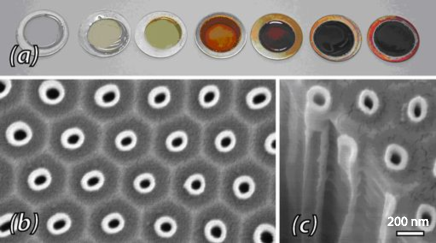
Figure 1: (Color online) Aspects of Fe₂O₃ nanotubes grown by atomic layer deposition (ALD) in a porous anodic alumina matrix. (a) Macroscopic view of the samples, consisting of a circular porous anodic alumina (AA) membrane containing the embedded tubes, surrounded by an outer circle of Al metal of 2 cm outer diameter; the tubes in the samples from left to right have walls of increasing thickness, approximately 0, 1, 2, 4, 8, 12, and 16 nm, respectively (AA obtained according to Method A, ALD performed by Method I). (b, c) Scanning electron micrographs (SEM) of tubes embedded in the porous alumina matrix, observed in top view and at an angle at a break in the sample, respectively; the scale bar represents 200 nm (AA obtained according to Method B, ALD performed by Method II).

Figure 2: Transmission electron micrographs (TEM) of isolated tubes from the alumina matrix, with walls of increasing thicknesses, approximately of 1(a), 5 (b), and 13 (c) nm, respectively; the scale bar represents 50 nm (AA obtained according to Method A, ALD performed by Method II).

In a series of Fe₃O₄ nanotube arrays of varying wall thickness $d_{w}$ (all other geometric parameters being kept constant), investigated by SQUID magnetometry, we observed a significant dependence of the coercivity and remanence upon the geometry. In particular, the coercive field $H_{c}$ can be tuned between 0 and 800 Oe (0 and 80 mT) approximately by properly adjusting $d_{w}$. Most curiously, the dependence of $H_{c}$ on $d_{w}$ is not monotonic - $H_{c}$ reaches its maximum at $d_{w}\approx 13$ nm and then decreases for further increases of the wall thickness (Figure 6b). We interpret this observation as arising from the coexistence of two distinct magnetization reversal modes in our system. Which of the two prevails in a given sample is uniquely determined by the geometric parameters of the tube array. Thus, the cusp in the $H_{c}\left(d_{w}\right)$ curve corresponds to the crossover between the two modes of magnetization reversal. The following paragraphs detail the theoretical treatment of the two modes.

III Two magnetization reversal modes

For isolated magnetic nanotubes, the magnetization reversal, that is, the change of the magnetization from one of its energy minima ($\mathbf{M}=M_{0}$ $\mathbf{\hat{z}}$) to the other ($\mathbf{M}=-M_{0}$ $\mathbf{\hat{z}}$), can occur by one of only two idealized mechanisms, the Vortex mode (V), whereby spins in rotation remain tangent to the tube wall, or the Transverse mode (T), in which a net magnetization component in the ($x$, $y$) plane appears. LAE+07 In both cases, a domain boundary appears at one end of the tube and propagates towards the other, as illustrated in Fig. 3. Starting from the equations presented by Landeros et al, LAE+07 we can calculate the zero-field energy barrier as well as the width of the domain boundary for each reversal mode as a function of the tube thickness, $d_{w}$. Figure 4a, 4b, and 4c present our results for Fe₃O₄ nanotubes using $M_{0}=4.8\times 10^{5}$ A/m³ and the stiffness constant $A=10^{-11}$ J/m. Ohandley00 Figure 4a witnesses a crossover at $d_{w}\approx 20$ nm, showing that the V mode is more stable for thinner tubes, whereas thicker tube walls favor the T mode. This result can be qualitatively explained as follows. A very thin tube should behave as a (rolled-up) thin film, in which the magnetic moments always tend to remain within the plane of the film. Conversely, tubes of large wall thicknesses approach the case of wires: surface effects are less crucial, but interactions between diametrically opposed regions become more important.

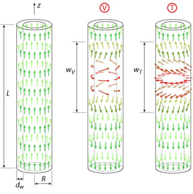
Figure 3: (Color Online) Geometric parameters and magnetization reversal modes in nanotubes. Arrows represent the orientation of magnetic moments within the tube. Left: A magnetically saturated tube ($\mathbf{M}=M_{0}$ $\mathbf{\hat{z}}$), with its geometric parameters, length $L$, radius $R$, wall thickness $d_{w}$. Center: A tube during the magnetization reversal from $M_{0}$ $\mathbf{\hat{z}}$ to $-M_{0}$ $\mathbf{\hat{z}}$ via a vortex mode, V; the domain boundary, of thickness $w_{V}$, migrates upwards. Right: The equivalent situation by means of a transverse reversal mode, T, with a domain boundary of thickness $w_{T}$.

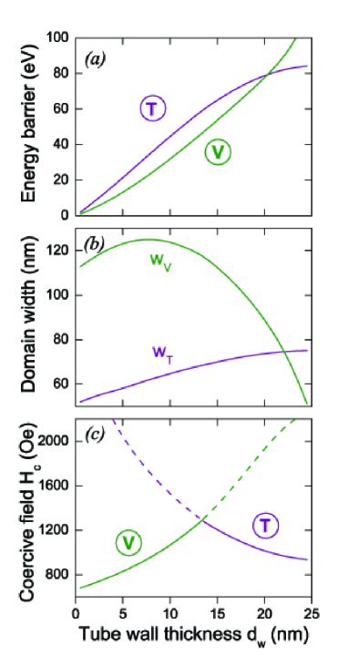
Figure 4: (Color online) Energy barrier (a) and domain boundary width (b) as a function of tube wall thickness for the V (green) and T (purple) modes of magnetization reversal. (c) Coercive fields obtained from Eqs. (1) and (2) for the V and T modes, (respectively shown in green and purple) for tube wall thicknesses varying between 0.5 and 24.5 nm. The dashed lines of the curves have no physical meaning. We have used $R=25$ nm

The presence of a crossover in Fig. 4a allows us to expect a transition from the V to the T reversal mode with increasing values of $d_{w}$. However, the curves cannot give the coercive field values directly because energies represent the difference between a completely saturated state and one with a domain boundary in the middle of the tube. Magnetization reversal, however, is initiated with a domain boundary at one end of the tube, a configuration that corresponds to a lower magnetic energy. From Fig. 4b we observe changes in boundary widths between 50 and 120 nm as a function of $d_{w}$. A crossover is found, corresponding to the one that appears between the energy curves. We shall now proceed to calculate the switching field of an isolated magnetic nanotube assuming that the magnetization reversal is driven by means of one of the two previously presented modes. coercivity

III.1 Coercive fields

For the T mode, the coercive field, $H_{n}^{T}$, can be approximated by an adapted Stoner-Wohlfarth model SW48 in which the length of the coherent rotation is replaced by the width of the domain boundary, $w_{T}$ (see Fig. 4b). Following this approach,

$$\frac{H_{n}^{T}}{M_{0}}=\frac{2K\left(w_{T}\right)}{\mu_{0}M_{0}^{2}}\ ,$$ (1)

where $K\left(l\right)=\frac{1}{4}\mu_{0}M_{0}^{2}\left(1-3N_{z}\left(l\right)\right)$ and $N_{z}\left(l\right)$ corresponds to the demagnetizing factor along $z$, given by $N_{z}\left(l\right)=\frac{2R}{\left(1-\beta^{2}\right)l}\int_{0}^{\infty}\frac{dq}{q^{2}}\left(J_{1}\left(q\right)-\beta J_{1}\left(q\beta\right)\right)^{2}\left(1-e^{-q\frac{l}{R}}\right)$, with $\beta=1-\frac{d_{w}}{R}$.

For the V mode we use an expression for the nucleation field obtained by Chang et al. CLY94 When an external field with magnitude equal to the nucleation field is applied opposite to the magnetization of the tube, infinitesimal deviations from the initially saturated state along the tube axis appear. The form of these deviations is determined by the solution of a linearized Brown’s equation. AS58 Furthermore, it has been shown numerically that the solution of this Brown’s equation is not a stable solution to the full nonlinear equation at applied fields larger than the nucleation field, and then the only possible stable states are those with uniform alignment along the axis. BB92 ; Brown58 Thus, the magnetization is assumed to reverse completely at the nucleation field. For an infinite tube, the nucleation field for the V mode, $H_{n}^{V}$, is given by

$$\frac{H_{n}^{V}}{M_{0}}=\alpha\left(\beta\right)\frac{L_{ex}^{2}}{R^{2}}\ ,$$ (2)

with $L_{ex}=\sqrt{2A/\mu_{0}M_{0}^{2}}$ and $\alpha\left(\beta\right)\equiv q^{2}$, where $q$ satisfies the condition

$$\frac{qJ_{0}\left(q\right)-J_{1}\left(q\right)}{qY_{0}\left(q\right)-Y_{1}\left(q\right)}=\frac{\beta qJ_{0}\left(\beta q\right)-J_{1}\left(\beta q\right)}{\beta qY_{0}\left(\beta q\right)-Y_{1}\left(\beta q\right)}\ .$$ (3)

Here $J_{p}\left(z\right)$ and $Y_{p}\left(z\right)$ are Bessel functions of the first and second kind, respectively. Equation (3) has an infinite number of solutions, and the physically correct solution is the smallest one.

Figure 4c illustrates the coercive field of an isolated tube with $d_{w}$ varying from $0.5$ to $24.5$ nm. We can observe a crossing of the two curves at $d_{w}=13$ nm approximately, corresponding to a magnetization reversal for which both V and T mechanisms are possible at the same coercive field. At other given values of $d_{w}$, the system will reverse its magnetization by whichever mode opens an energetically accessible route first, that is, by the mode that offers the lowest coercivity. Therefore, the curve of coercivity vs. $d_{w}$ is the solid one, and the dotted sections of curves have no physical meaning. Thus, our Fe₃O₄ tubes will reverse their magnetization by the V mode for $d_{w}<13$ nm, and by the T mode for $d_{w}>13$ nm. Our calculations for an isolated tube reproduce the non-monotonic behavior of the coercive field as a function of the wall thickness experimentally observed, with a transition between two different modes causing a cusp at $d_{w}^{V-T}=13$ nm (with $d_{w}^{V-T}$ the thickness at which the transition occurs). However, the absolute values computed for the coercivity are greater than the experimental data.

III.2 Effect of the stray field

We ascribe such difference between calculations and experimental results to the interaction of each tube with the stray fields produced by the array - an effective antiferromagnetic coupling between neighboring tubes, which reduces the coercive field (as previously demonstrated in the case of nanowires; see Fig. 6a). Hertel01 ; VPH+04 ; BAA+06 ; ELP+08 In these interacting systems, the process of magnetization reversal can be viewed as the overcoming of a single energy barrier, $\Delta E$. In an array with all the nanotubes initially magnetized in the same direction, the magnetostatic interaction between neighboring tubes favours the magnetization reversal of some of them. A reversing field aligned opposite to the magnetization direction lowers the energy barrier, thereby increasing the probability of switching. The dependence of the applied field on the energy barrier is often described Sharrock94 by the expression

$$\Delta E=U\left(1-\frac{H}{H_{0}}\right)^{2}\ ,$$

where $H$ is the applied field, and $H_{n}$ denotes the intrinsic coercivity of an isolated wire. For single-domain particles having a uniaxial shape anisotropy, the energy barrier at zero applied field, $U$, is just the energy required to switch by coherent rotation, $K\left(L\right)$. If we assume that the switching field $H_{s}$ is equal to $H_{c}$, then

$$H_{c}=H_{n}^{i}-H_{int},$$ (4)

where $H_{n}^{i}$ denotes the intrinsic coercivity $H_{n}^{V}$ or $H_{n}^{T}$ of an isolated tube, and $H_{int}$ corresponds to the stray field induced within the array given by

$$\frac{H_{int}}{M_{0}}=\frac{2K\left(L\right)}{\mu_{0}M_{0}^{2}}\left(\frac{\varepsilon\left|\tilde{E}_{int}\left(s\right)\right|}{K\left(L\right)}\right)^{1/2}\ ,$$ (5)

In the previous equation we have assumed that the reversal of individual nanotubes produces a decrease of the magnetostatic energy $E_{int}$ that equals the magnetic anisotropy barrier $\Delta E$. Besides, $\varepsilon$ is an adjustable parameter that depends on the distribution of magnetic tubes in space and on the long-distance correlation among the tubes. The value of $\varepsilon$ can not be obtained from first principles, although values between unity and some tens could be a reasonable estimate for this quantity. ACT+01 Besides, $\tilde{E}_{int}\left(s\right)$ is the magnetostatic interaction between two nanotubes separated by a distance $s$. Such interaction can be calculated by considering each tube homogeneously magnetized and is given by

$$\tilde{E}_{int}\left(s\right)\equiv\frac{E_{int}\left(s\right)}{V}=\frac{2\mu_{0}M_{0}^{2}R}{\left(1-\beta^{2}\right)L}\\ \cdot\int_{0}^{\infty}\frac{dq}{q^{2}}J_{0}\left(q\frac{s}{R}\right)\left(J_{1}\left(q\right)-\beta J_{1}\left(q\beta\right)\right)^{2}\left(1-e^{-q\frac{L}{R}}\right).$$

The resulting curve $H_{int}(d_{w})$ $(\varepsilon=20)$ is illustrated in the top panel of Fig. 6a. The stray fields produced by an array of nanotubes are significant for the experimentally investigated tubes, being on the order of $350$ Oe for $d_{w}=5$ nm to $580$ Oe by $d_{w}=21$ nm.

III.3 Results

The hysteresis loop in normalized axis of a sample of $L=3$ $\mu$m, $R=50$ nm, and $d_{w}=13$ nm is presented in Fig. 5. In this loop we have subtracted a paramagnetic background. Our results are combined in the lower panel of Fig. 6. Experimental data for the coercivity of the array are depicted by dots. In this figure we can observe the strong dependence of the coercivity as a function of the tube wall thickness, evidencing clearly the existence of a maximum. Also the coercivities of an isolated tube and interacting array obtained from our calculations are depicted in the same figure by dashed and solid lines, respectively. We consider $\varepsilon=20$ in Eq. (4). Note the good agreement between experimental datapoints and analytical results for interacting arrays for $d_{w}\geq 8$ nm.

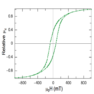
Figure 5: (Color online) Magnetic hysteresis loop measured for $L=3$ $\mu$m, $R=50$ nm, and $d_{w}=13$ nm (after substraction of a paramagnetic background and normalization.)

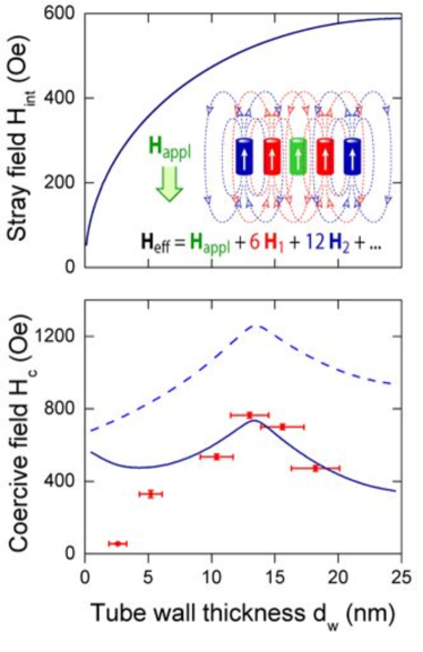
Figure 6: (Color online) (Upper panel) Stray field $H_{int}$ calculated from Eq. (5) as a function of the tube wall thickness $d_{w}$. As shown in the inset, in an array, contributions from the six nearest neighbors, the twelve second-degree neighbors, and the tubes situated farthest away from the probe tube combine to form the so-called stray field, which is in the $-z$ direction and therefore drives the probe tube to reverse its magnetization at smaller absolute values of the applied field than it would if it were isolated. (Lower panel) Coercive field as a function of the tube wall thickness for Fe₃O₄ nanotubes. The red (dark gray) dots correspond to the data measured in ordered arrays, the light blue (dashed) line represents the values calculated for an isolated tube, and the deep blue (solid) curve is calculated for an array of nanotubes. Parameters: $R=25$ nm, $L=3$ $\mu$m and $D=105$ nm. Equation (5) was used with $\varepsilon=20$.

The deviation of the experimental datapoints from the calculated curve for $d_{w}\leq 8$ nm likely originates from the structural imperfections of the tubes. Deposition of the magnetic material may lead to granular walls at the initial stages of the growth, whereas further increases in wall thickness accounted in a smoothening. Other factors not account for in our theoretical model include thermal instability, which has a stronger effect in thinner particles, possible shape irregularities, Braun93 and the finite length of the tubes.

The results presented above may be generalized. We now proceed to investigate how the curve will be affected by changes in the tube radius, $R$, and of the material, by considering the trajectories of the transition thickness, $d_{w}^{V-T}$. Such trajectories are shown in Fig. 7 for four different materials. In the range of parameters considered, we observe that an increase of the external radius, $R$, results in an increase of the transition thickness, $d_{w}^{V-T}$. Furthermore, the curves $d_{w}^{V-T}\left(R\right)$ are steeper for materials with longer exchange lengths. Figure 7 can also be interpreted as a phase diagram, in that each line separates the T mode of magnetization reversal, which prevails in the upper left region of the ($R$, $d_{w}$) space, from the V mode, found in the lower right area.

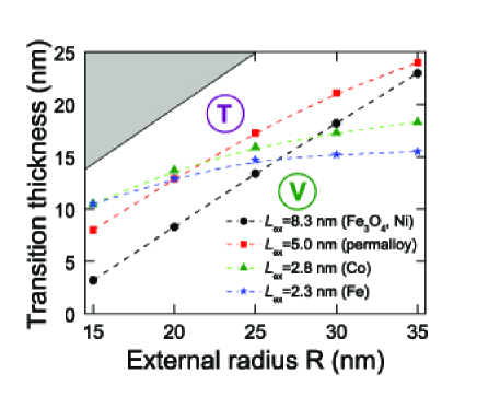
Figure 7: (Color online) Trajectories of the transition thickness, $d_{w}^{V-T}$, as a function of $R$, for Fe₃O₄ (circles, Permalloy (squares), Co (triangles) and Fe (stars). Because of the similarity of Ni and Fe₃O₄ in terms of their magnetic parameters, the results presented for Fe₃O₄ approximate the case of Ni tubes as well.

IV Conclusions

In conclusions, by means of simple models for the domain boundary that appears during the magnetization reversal in nanotubes, we can calculate the coercive field in ordered arrays of ferromagnetic nanotubes as a function of the tube wall thickness and the radius. A transition between two different modes of magnetization reversal, from a vortex boundary, in thin tubes, to a transverse boundary, in thick tubes, is responsible for the non-monotonic behavior of the coercivity as a function of wall thickness experimentally observed. The effect of the stray field originating from the magnetostatic interactions between the tubes of the array must be included to obtain a quantitative agreement between experimental and theoretical results. Because of its long range, the magnetostatic interaction strongly influences the coercivity of the array. Finally, the presence of a coercivity maximum at a certain optimum wall thickness should be a quite general phenomenon, observable for a variety of ferromagnetic materials and of tube radii. Experimental work remains to be done in order to validate these predictions.

- (1) S. Sun, C. B. Murray, D. Weller, L. Folks, and A. Moser, Science 287, 1989 (2000).
- (2) R. H. Koch, J. G. Deak, D. W. Abraham, P. L. Trouilloud, R. A. Altman, Yu Lu, W. J. Gallagher, R. E. Scheuerlein, K. P. Roche, and S. S. P. Parkin, Phys. Rev. Lett. 81, 4512-4515 (1998).
- (3) R. P. Cowburn, D. K. Koltsov, A. O. Adeyeye, M. E. Welland, and D. M. Tricker, Phys. Rev. Lett. 83, 1042-1045 (1999).
- (4) S. A. Wolf, D. D. Awschalom, R. A. Buhrman, J. M. Daughton, S. von Molnar, M. L. Roukes, A. Y. Chtchelkanova, and M. Treger, Science 294, 1488-1495 (2001).
- (5) Th. Gerrits, H. A. M. van den Berg, J. Hohlfeld, L. Bar, and Th. Rasing, Nature 418, 509-512 (2002).
- (6) D. F. Emerich, and C. G. Thanos, Expert Opin. Biol. Ther. 3, 655-663 (2003).
- (7) V. F. Puntes, K. M. Krishnan, and A. P. Alivisatos, Science 291, 2115 (2001).
- (8) W. Wernsdorfer, B. Doudin, D. Mailly, K. Hasselbach, A. Benoit, J. Meier, J. -Ph. Ansermet, and B. Barbara, Phys. Rev. Lett. 77, 1873-1876 (1996).
- (9) D. Atkinson, A. Allwood, G. Xiong, M. D. Cooke, C. C. Faulkner, and R. P. Cowburn, Nature Mat. 2, 85-87 (2003).
- (10) L. Thomas, M. Hayashi, X. Jiang, R. Moriya, C. Retener, and S. S. P. Parkin, Nature 443, 197-200 (2006).
- (11) R. P. Cowburn, Nature 448, 544-545 (2007).
- (12) M. Eisenstein, Nature Methods 2, 484 (2005).
- (13) Yumei Chen, Fan Yang, Yu Dai, Weiqi Wang, and Shengli Chen, J. Phys. Chem. C 112, 1645-1649 (2008).
- (14) S. Iijima, Nature 354, 56 (1991).
- (15) D. T. Mitchell, S. B. Lee, L. Trofin, N. Li, T. K. Nevanen, H. Soderlund, and C. R. Martin, J. Am. Chem. Soc. 124, 11864-11865 (2002).
- (16) S. J. Son, J. Reichel, B. He, M. Schushman, and S. B. Lee, J. Am. Chem. Soc. 127, 7316-7317 (2005).
- (17) K. Nielsch, F. J. Casta–o, S. Matthias, W. Lee, and C. A. Ross, Adv. Eng. Mater. 7, 217 (2005).
- (18) Z. K. Wang, H. S. Lim, H. Y. Liu, S. C. Nq, M. H. Kuok, L. L. Tay, D. J. Lockwood, M. G. Cottam, K. L. Hobbs, P. R. Larson, J. C. Keay, G. D. Lian, and M. B. Johnson, Phys. Rev. Lett. 94, 137208 (2005).
- (19) T. Feifei, G. Mingyun, J. Yuan, Z. Jianmin, X. Zheng, and X. Ziling, Adv. Mater. 18, 2161 (2006).
- (20) J. Escrig, P. Landeros, D. Altbir, E. E. Vogel, and P. Vargas, J. Magn. Magn. Mater. 308, 233-237 (2007).
- (21) Y. C. Sui, R. Skomski, K. D. Sorge, and D. J. Sellmyer, Appl. Phys. Lett. 84, 1525 (2004).
- (22) J. Bachmann, J. Jing, M. Knez, S. Barth, H. Shen, S. Mathur, U. Gosele, and K. Nielsch, J. Am. Chem. Soc. 129, 9554-9555 (2007).
- (23) That is, the x and y intercepts of the magnetic hysteresis curve, respectively: the remanence is the fraction of the saturated (maximum) magnetization that remains once the applied magnetic field has been turned off, and the coercive field is the absolute value of the magnetic field applied in the direction needed to reduce the magnetization in the direction to zero (in other words, to erase the remanence).
- (24) S. Goolaup, N. Singh, A. O. Adeyeye, V. Ng, and M. B. Jalil, Eur. Phys. J. B 44, 259 (2005).
- (25) H. Masuda, and K. Fukuda, Science 266, 1466-1468 (1995).
- (26) K. Nielsch, J. Choi, K. Schwim, R. B. Wehrspohn, and U. Gosele, Nano Lett. 2, 677-680 (2002).
- (27) R. L. Puurunen, Appl. Phys. Lett. 97, 121301 (2005), and references therein.
- (28) See for example, B. S. Lim, A. Rahtu, and R. G. Gordon, Nature Mat. 2, 749-754 (2003).
- (29) P. Landeros, S. Allende, J. Escrig, E. Salcedo, D. Altbir, and E. E. Vogel, Appl. Phys. Lett. 90, 102501 (2007).
- (30) R. C. O’Handley, Modern Magnetic Materials, Wiley, New York (2000).
- (31) Strictly speaking, the determination of the coercivity actually requires an analysis of the nonlinear regime, which is lacking at this point. Landeros et al. [29] demonstrated that the coherent mode is present only in very short tubes, and that if there is no other switching mode than V and T, results for the nucleation field corresponds to the coercivity.
- (32) E. C. Stoner, and E. P. Wohlfarth, Philos. Trans. R. Soc. London, Ser. A240, 599 (1948). [Reprinted in IEEE Trans. Magn. 27, 3475 (1991)].
- (33) Ching-Ray Chang, C. M. Lee, and Jyh-Shinn Yang, Phys. Rev. B 50, 6461 (1994).
- (34) A. Aharoni, and S. Shtrikman, Phys. Rev. 109, 1522 (1958).
- (35) J. S. Broz, and W. Baltensperger, Phys. Rev. 45, 7307 (1992).
- (36) W. F. Brown, Jr., J. Appl. Phys. 29, 470 (1958).
- (37) R. Hertel, J. Appl. Phys. 90, 5752 (2001).
- (38) M. Vazquez, K. Pirota, M. Hernandez-Velez, V. M. Prida, D. Navas, R. Sanz, F. Batallan, and J. Velazquez, J. Appl. Phys. 95, 6642 (2004).
- (39) M. Bahiana, F. S. Amaral, S. Allende, and D. Altbir, Phys. Rev. B 74, 174412 (2006).
- (40) J. Escrig, R. Lavin, J. L. Palma, J. C. Denardin, D. Altbir, A. Cortes, and H. Gomez, Nanotechnology 19, 075713 (2008).
- (41) Sharrock M P 1994 J. Appl. Phys. 76 6413-6418.
- (42) Paolo Allia, Marco Coisson, Paola Tiberto, Franco Vinai, Marcelo Knobel, M. A. Novak, and W. C. Nunes, Phys. Rev. B 64, 144420 (2001).
- (43) Hans-Benjamin Braun, Phys. Rev. Lett. 71, 3557 (1993).