figurec

Topological Schrödinger cats: Non-local quantum superpositions of topological defects

Topological defects (such as monopoles, vortex lines, or domain walls) mark locations where disparate choices of a broken symmetry vacuum elsewhere in the system lead to irreconcilable differences Mermin79-1 ; Michel80-1 . They are energetically costly (the energy density in their core reaches that of the prior symmetric vacuum) but topologically stable (the whole manifold would have to be rearranged to get rid of the defect). We show how, in a paradigmatic model of a quantum phase transition, a topological defect can be put in a non-local superposition, so that – in a region large compared to the size of its core – the order parameter of the system is “undecided” by being in a quantum superposition of conflicting choices of the broken symmetry. We dub such a topological Schrödinger cat state a ‘Schrödinger kink’, and devise a version of a double-slit experiment suitable for topological defects to describe one possible manifestation of the phenomenon. Coherence detectable in such experiments will be suppressed as a consequence of interaction with the environment. We analyze the environment-induced decoherence and discuss its role in symmetry breaking.

Topological defects are the epitome of locality. An example of a defect occurs in the quantum Ising model where a lattice of spins interact ferromagnetically with their nearest neighbors, i.e., the Hamiltonian contains an interaction of the form $-\sigma_{n}^{z}\sigma_{n+1}^{z}$ for the $n^{th}$ spin on the lattice. The entire collection of spins achieves its lowest energy when they are all aligned. However, there are two choices for this lowest energy state, $|\cdots\uparrow\uparrow\uparrow\uparrow\cdots\rangle$ or $|\cdots\downarrow\downarrow\downarrow\downarrow\cdots\rangle$. Both are energetically identical but each of them breaks the symmetry of the Hamiltonian, which has no preference between “up” and “down”.

Figure 1: A Schrödinger kink in a quantum Ising chain. (a) A topological defect in a non-local superposition and (b) The analogue of a double-slit experiment. A double-well potential (left) is used to create a superposition of a topological defect, such as a Schrödinger kink described by wavefunction representing a superposition of two locations (here we plot the corresponding probability distribution in space). The analogy with the humane version of the Schrödinger cat experiment is obvious. To carry out the double slit experiment, the two potential wells are eliminated, allowing the defect to move. In isolation, the two wavepackets emerging from the “slits” interfere creating fringes of high and low probability for the location of the kink. However, when the system interacts with the environment, such a superposition will decohere at a rate proportional to the distance $L$ – the unzipped part of the chain shown in (a), which corresponds to the size of the Schrödinger kink – resulting in a classical distribution for the defect.

A configuration that includes topological defects could arise, for example, in a driven phase transition, i.e., “a quench”. In the Ising model, a quench can be induced when the transverse field strength $g$ is changed in the Hamiltonian

$$H=-\sum_{n}\left(g\sigma_{n}^{x}+\sigma_{n}^{z}\sigma_{n+1}^{z}\right).$$ (1)

When the external field is strong enough ($g\gg 1$), it “wins” and all spins align with $\sigma^{x}$. A decrease in $g$, however, will lead to a phase transition at $g=1$ with the symmetry breaking term $-\sigma_{n}^{z}\sigma_{n+1}^{z}$ trying to align all the spins in their $z$-direction.

The choice of whether the spins will point up or down is made locally. As a result of causality and the finite speed at which signals propagate, the size of these domains will be determined by rate of change of $g$ Kibble76-1 ; Kibble80-1 ; Zurek85-1 ; Zurek93-1 ; Zurek96-1 ; Kibble07-1 . This will lead to configurations, such as $|\cdots\uparrow\uparrow\downarrow\downarrow\cdots\rangle$, where the topological defect marks the location of a “switch” from one broken symmetry ground state to the other. In this one-dimensional example, the defect is a kink (a domain wall), but, in a sense, all the topological defects (monopoles, vortex lines, and so on) that exist in higher dimensions “look the same”. A discussion of the consequences of this process for the post-transition state is beyond the scope of this work (but see, e.g., Refs. Anglin99-1, ; Zurek05-1, ; Dziarmaga05-1, ). We only note that the density of the resulting kinks will be finite.

The quantum Ising model quenches a state according to Hamiltonian (1) so, when $g$ is changed in time, superpositions of different locations of a kink (e.g., $\alpha|\cdots\uparrow\uparrow\downarrow\downarrow\downarrow\downarrow\cdots\rangle+\beta|\cdots\uparrow\uparrow\uparrow\downarrow\downarrow\downarrow\cdots\rangle+\gamma|\cdots\uparrow\uparrow\uparrow\uparrow\downarrow\downarrow\cdots\rangle$) are allowed, and, indeed, inevitable Zurek05-1 ; Dziarmaga05-1 . Spreading of a localized kink will come about as a consequence of the kinetic term, $g\sigma_{n}^{x}$, in equation (1). A convenient setting to investigate its effect is offered by a slight modification of the original Hamiltonian, so that the Ising interaction between a selected pair of sites, $n_{0},n_{0}+1$, is $-\left(1-w\right)\sigma_{n_{0}}^{z}\sigma_{n_{0}+1}^{z}$ with $w>0$, which differs somewhat from the uniform coupling of $-\sigma_{n}^{z}\sigma_{n+1}^{z}$. This difference means that the kink is energetically less expensive when localized between those two selected sites. The decrease in the coupling constant by $w$ creates a local “potential well” that binds this kink. On the other hand, the kinetic term will delocalize the kink so that the quantum wavefunction of the kink will have the form

$$\psi_{n}\propto e^{-\gamma_{0}\left|n-n_{0}\right|},$$ (2)

where $\psi_{n}$ is the amplitude for the kink to be on the link $n$ between sites $n$ and $n+1$, $n_{0}$ is the location of the potential well, and $\gamma_{0}=\sinh^{-1}\left(w/g\right)$ is the inverse decay length of the wavepacket. One can imagine measurements that will reveal such a non-local wavepacket – a kink in a superposition of many locations. We emphasize that the half-width of this wavepacket is not the size of the kink: The kink is a local object with a size given by the healing length that – in the quantum Ising model far away from the critical point – is given by the lattice spacing of the neighboring spins. The spread in equation (2) represents a superposition of many possible locations of the kink, which is bound to the weak link between sites $n_{0}$ and $n_{0}+1$, but nevertheless has some spatial extent.

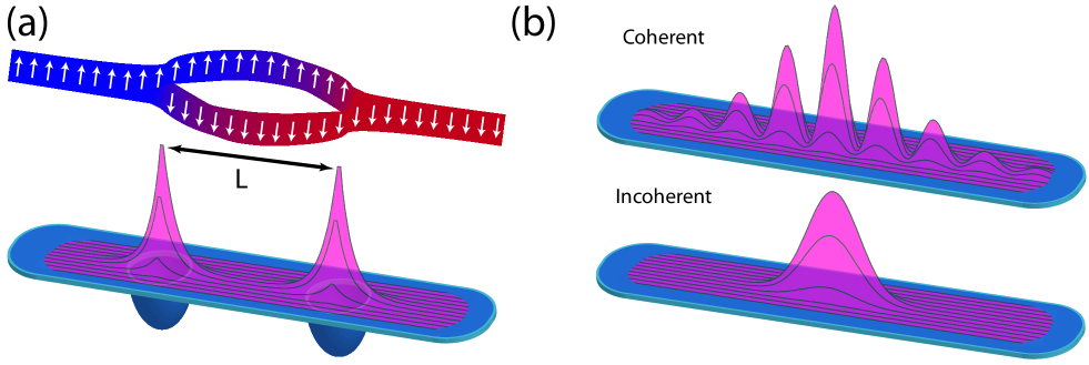
A tell-tale signature of quantum coherence is an interference pattern. To see whether a defect can interfere with itself, we devise an analogue of the double-slit experiment (see Figure 1 for a schematic). To this end, the local value of the Ising coupling can be depressed by $w$ at two locations separated by $L$ sites. The two links that bind the same kink initially are analogues of the slits in the double-slit experiment. To achieve a situation where the kink is “both here and there” one can start it on one of the two binding sites and evolve so that tunneling of the kink will result in the state

$$|\cdots\uparrow\uparrow\uparrow\overbrace{\downarrow\downarrow\cdots\downarrow\downarrow}^{L}\downarrow\downarrow\downarrow\cdots\rangle$$

$$+ |\cdots\uparrow\uparrow\uparrow\underbrace{\uparrow\uparrow\cdots\uparrow\uparrow}_{L}\downarrow\downarrow\downarrow\cdots\rangle,$$ (3)

where we have ignored the spread of the wavepacket for simplicity. This is also illustrated in Figure 1(a), where the superposition of the kink forms a “scar” in the orientation of the spins, “unzipping” the $L$-sized region of the spin chain in Fig. 1.

This is not the only way to create a “Schrödinger kink” state. As we shall see later, one can also start with a kink localized state on a single “weak link”. If the kink is released symmetrically, it will travel both left and right.

Figure 2: Interference patterns after a Schrödinger kink is released. (a) Time evolution of the Schrödinger kink for $L=50$ and $2w=0.3g$ results in an interference pattern (highlighted in red at the final time). (b) Interference pattern in the long time limit ($gt=1000$) for $L=100$ and $2w=0.3g$. (c) Interference pattern in the long time limit ($gt=1000$) for $L=50$ and $2w=0.3g$. In (b) and (c), the exact data is shown as black crosses and equation (4) is shown as the blue line. As the distance between the two “slits” where the kink is trapped decreases so does the number of interference fringes.

The double-slit experiment can be now conducted starting from this initial configuration by eliminating the two weak links. The kink is then no longer bound by the “double-well” potential: The Schrödinger kink propagates in accord with the Schrödinger equation and the two components of the wavepacket run into each other. If coherence was properly preserved between them, this will lead to an interference pattern.

Preserving phase coherence is crucial if the resulting interference pattern is to be seen in experiments. Trivial reasons for loss of coherence – such as an imprecise implementation of the two weak links – will have to be eliminated. However, the fundamental reason for the loss of coherence is environment-induced decoherence Zurek91-1 ; Paz00-1 ; Zurek03-1 ; Joos03-1 ; Schlosshauer08-1 ; Nielsen00-1 . It is important to understand its causes and its nature, as it is not just an impediment to creating superpositions described above, but the prevailing reason why topological defects we encounter are always localized.

Decoherence is caused by the interaction of individual spins with the environment $\mathcal{E}$. The pointer states Zurek81-1 ; Zurek82-1 entangle least with the environment. They are selected with the help of the interaction Hamiltonian. For instance, an individual spin $|\uparrow\rangle$ can leave a different imprint on $\mathcal{E}$ than the spin $|\downarrow\rangle$, i.e., $\left(\alpha|\uparrow\rangle+\beta|\downarrow\rangle\right)|\mathcal{E}_{0}\rangle\to\alpha|\uparrow\rangle|\mathcal{E}_{\uparrow}\rangle+\beta|\downarrow\rangle|\mathcal{E}_{\downarrow}\rangle$. The overlap $\langle\mathcal{E}_{\uparrow}|\mathcal{E}_{\downarrow}\rangle$ determines the decoherence factor, with $\langle\mathcal{E}_{\uparrow}|\mathcal{E}_{\downarrow}\rangle=0$ corresponding to the complete loss of coherence. The decoherence factor controls size of the off-diagonal terms in the density matrix. When they disappear, quantum coherence between $|\uparrow\rangle$ and $|\downarrow\rangle$ is lostZurek91-1 ; Paz00-1 ; Zurek03-1 ; Schlosshauer08-1 .

Returning to our Schrödinger kink, we note that when two locations are separated by $L$ spins, equation (3), the decoherence process will take place simultaneously in all $L$ spins. Assuming that each spin leaves its own imprint will lead to a decoherence factor that scales as $\langle\mathcal{E}_{\uparrow}|\mathcal{E}_{\downarrow}\rangle^{L}$, where $L$ is the number of unzipped spins – the spatial extent of the superposition of the “Schrödinger kink”. This exponential scaling with the extent of the superposition is intuitively obvious: We do not have to assume any specific model for the decoherence. All that is needed is the familiar assumption (see, e.g., modeling of errors in quantum error correction Nielsen00-1 ) that individual spins (or local regions) affect the environment individually.

This assumption suffices to show that the decoherence rate is proportional to the “size”, $L$, of the superposition. That is, decoherence time is $\tau_{dec}\sim 1/L$. This conclusion is confirmed by calculations employing a master equation (see the Supplemental Information). One can generalize this intuition to superpositions of topological defects in higher dimensions by noting that it is the volume of the system – the size of the domain that is suspended in indecision between two broken symmetry vacua – that is responsible for the decoherence rate.

Figure 3: A Schrödinger kink evolved in the presence of decoherence. (a) Time evolution for strong decoherence ($\Gamma=g/2$), $L=50$, and $2w=0.3g$, where the Schrödinger kink evolves into a (b) Gaussian mixture of locations (highlighted in red in (a)) at a later time, $gt=100$ (the black crosses are the exact data and the blue curve is the solution to the diffusion equation). (c) Under weak decoherence ($\Gamma=g10^{-3}/8$), the superposition is still visible at intermediate times, but the decoherence smoothes out the fringes (the black crosses are the exact data and the blue curve is the pure state solution convoluted with a Lorentzian).

Figure 4: A single kink evolved on a finite lattice with and without decoherence. (Left) Time evolution without decoherence on an $L=201$ site lattice and $2w=0.5g$. The kink travels outward on the lattice and after reflecting off the boundaries, it starts to interfere with itself. The leftmost panels show the self interference at two particular times. (Right) The same simulation except in the presence of weak decoherence ($\Gamma=3g\times 10^{-6}$). The kink can still interfere with itself, but eventually decoherence will suppress the superposition, attenuating the interference pattern. In the supplemental information, we show movies of the development of this interference pattern for different values of $w$.

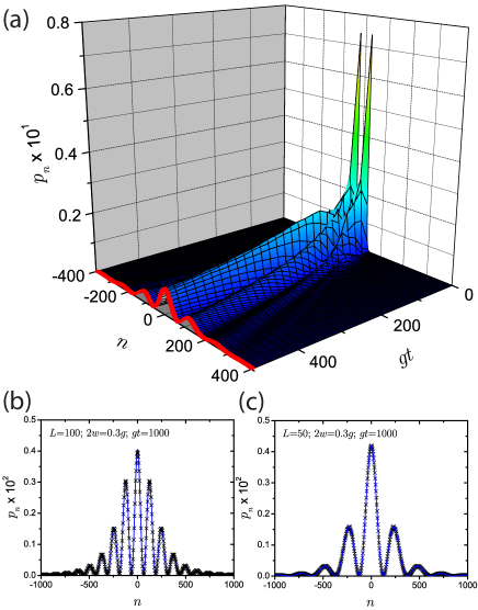
We now return to the Ising model. In the absence of decoherence, a well-defined interference pattern develops when the two initial components of the wavepacket run into each other (Fig. 2). As the distance, $L$, between these two components is increased, more fringes become visible (i.e., decreasing $L$ decreases the magnitude of the outer fringes), as seen by Figs. 2(b,c). This is demonstrated explicitly by the form of the fringes,

$$p_{n}\left(t\right)=\left|\psi_{n}\left(t\right)\right|^{2}\propto\frac{1+\cos\frac{\left(n-n_{0}-L/2\right)L}{2gt}}{\left[1+\frac{\left(n-n_{0}-L/2\right)^{2}}{\left(2\gamma_{0}gt\right)^{2}}\right]^{2}}.$$ (4)

This interference pattern is analogous to the one observed in the double-slit experiment. In the double-slit experiment the distance between fringes is $\lambda D/L$, where $L$ is the distance between the slits, $\lambda$ is the wavelength of light, and $D$ is the distance to the screen. For kinks, the distance traveled is $D=\upsilon_{k}t\approx 2gkt=2g\left(2\pi/\lambda\right)t$, where $\upsilon_{k}=d\omega/dk\approx 2gk$ is the group velocity of the kink for slow kinks that are generated when $w\ll 1$, as we assume in deriving Eq. (4) (the figures use $\upsilon_{k}=2g\sin k$, demonstrating that this assumption is sound). This linear approximation yields the fringe distance for kink interference $\lambda D/L=4\pi gt/L$, as given in equation (4). The height of the second peak relative to the first is $1/\left[1+4\pi^{2}/L^{2}\gamma_{0}^{2}\right]^{2}$. In effect, the linear approximation of $\upsilon_{k}=2g\sin k$ entitles one to think of kinks in a double slit experiment as one would think of, say, electrons or neutrons.

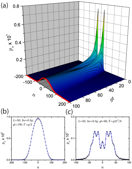
Decoherence suppresses interference. Figure 3(a,b) shows the evolution of the kink probability density (that determines the probability of finding a kink at a certain location) under strong decoherence. In presence of decoherence it evolves into a Gaussian form seen in Fig. 3(b). Even weak decoherence will attenuate interference. The decoherence time depends on $L$: Coherence disappears exponentially fast in $L$, the separation between components of the wavepacket. The evolution of the superposition under weak decoherence is shown in Fig. 3(c).

The double slit experiment for kinks we have just discussed has the advantage of a straightforward interpretation. The use of the coherent bi-local Schrödinger kink that is relatively weakly bound to the two sites allows one to linearize the dispersion relation and use $\upsilon_{k}=2gk$ for the kink velocity. This leads in turn to the simple form of the interference pattern, equation (4).

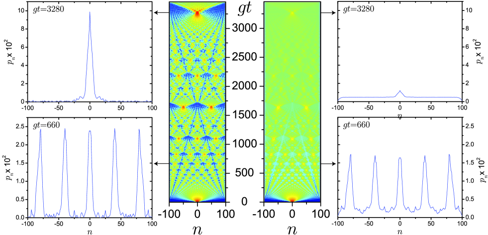
However, this ease of interpretation may come at the price of difficult implementation. In particular, preparing the initial bi-local kink wavepacket and maintaining coherence between its two pieces of the will be a challenge. A different version of Schrödinger kink that should be easier to implement is therefore illustrated in Fig. 4. Here the kink is initially bound to a specific link along the Ising chain. This kink trap is instantaneously turned off, which results in a coherent spreading of the wavepacket with a superposition of velocities and in both directions on the Ising chain.

As before, we are not satisfied with just creating a Schrödinger kink. One should confirm that quantum coherence is present. In Fig. 4 this is accomplished by reflecting the spreading wavepacket from the ends of the Ising chain. The time-evolving interference pattern is now more complicated than before, but – in absence of decoherence – it clearly exhibits quantum coherence that can be predicted by suitably “folding” the kink’s wavefunction upon itself. Decoherence (as expected) suppresses interference fringes over time: As with double slit analog, the decoherence strength will have to decrease as $\sim 1/L$, where $L$ is the support of the wavepacket, if coherence – and, hence, interference – is to survive.

The interference pattern in Fig. 4 bears the imprint of the dispersion relation on a lattice, $\omega=-2g\cos k$: When released, a tightly bound kink turns into a wavepacket that propagates as a Bessel function, $p_{n}\left(t\right)=\left|J_{n}\left(2gt\right)\right|^{2}$. Our kinks of both Fig. 4 and especially of Fig. 2 are relatively weakly bound. Therefore, the Bessel oscillation is suppressed – smoothed out by the non-local nature of the wavepacket that eliminates large $k$ contributions (see Supplementary Information). Nevertheless, small-scale jaggedness of the interference pattern visible in Fig. 4 (where $w$ is larger than in Fig. 2, and, therefore, the kink starts more tightly localized) is a remnant of these Bessel oscillations.

An obvious application of this observation is the “collapse” of the superposition of the broken symmetry vacua after a phase transition. For example, in the case of the quantum Ising model, the ferromagnetic ground state is a superposition of $|\uparrow\cdots\uparrow\rangle$ and $|\downarrow\cdots\downarrow\rangle$. The total number of spins, $N$, in the Ising chain is the size of the superposition (e.g., $|\uparrow\cdots\uparrow\rangle+|\downarrow\cdots\downarrow\rangle$), but this symmetric superposition will become a mixture of the two obvious broken symmetry states in a very short time, $\tau_{dec}\sim 1/N$. This is a simple and compelling explanation of the symmetry breaking that occurs whenever a phase transition starting from a symmetric vacuum takes place.

The effectiveness of decoherence in localizing topological defects provides novel insights into symmetry breaking dynamics. A phase transition leads to a single quasi-classical configuration pockmarked with topological defects: Decoherence is the final step in this process. It leads to the “collapse of the wavepacket” that initially contains all the possible broken-symmetry configurations.

In the end, only a simple quasi-classical configuration is in evidence. This is essentially the same course of events that takes place in quantum measurement Wheeler83-1 , where breaking of the unitary symmetry allows for a “collapse of the wavepacket”. Recent progress in emulating quantum Ising and other models Friedenauer08-1 ; Kim10-1 ; Schneider10-1 ; Bakr10-1 ; Lin11-1 ; Chen11-1 allows one to hope that experimental tests of “Schrödinger kinks” may become possible in the near future. Moreover, although models of superfluids do not allow one to develop and analyze microscopic quantum theories of double-slit experiments for the relevant topological defects with the detail we have presented above for kinks, experiments involving the generation and manipulation of such defects in, for example, gaseous Bose–Einstein condensates allow one to hope that testing of ‘topological Schrödinger cats’ involving vortex lines or solitons may also be possible.

Supplemental Information

Interference fringes

We are interested in the one-kink subspace of the Hamiltonian (1) spanned by states

$$|n\rangle=|\uparrow\uparrow\cdots\uparrow_{n}\downarrow_{n+1}\cdots\downarrow\downarrow\rangle,$$ (5)

which have a kink on the link between sites $n,n+1$. We can confine to this subspace when $g^{2}\ll 1-w$ and the magnetic field $g$ is too weak to mix with the subspaces of $3,5,..$ kinks. When there is only one weaker link, then a stationary state $|\psi\rangle=\sum_{n}\psi_{n}|n\rangle$ satisfies a Schrödinger equation

$$E\psi_{n}=-g\left(\psi_{n+1}+\psi_{n-1}\right)-2w\delta_{n_{0},n}\psi_{n}.$$ (6)

The magnetic field $g$ provides a hopping term between nearest neighbor links and the weaker link of strength $1-w$ results in a trapping potential of strength $2w$ localized on the link $n_{0}$. This potential has one localized bound state

$$\psi_{n}=\cosh\left(\gamma_{0}\right)e^{-\gamma_{0}\left|n-n_{0}\right|},$$ (7)

where $\gamma_{0}=\sinh^{-1}(w/g)$, with energy $E_{0}=-2g\cosh(\gamma_{0})\leavevmode\nobreak\ =\leavevmode\nobreak\ -2\sqrt{g^{2}+w^{2}}.$

When there are two weaker links, $n_{0}$ and $n_{0}+L$, the Schrödinger equation

$$E\psi_{n}=-g\left(\psi_{n+1}+\psi_{n-1}\right)-2w\left(\delta_{n_{0},n}+\delta_{n_{0}+L,n}\right)\psi_{n}$$ (8)

has two bound states

$$\psi_{n}^{\mp}\propto e^{-\gamma\left|n-n_{0}\right|}\mp e^{-\gamma\left|n-n_{0}-L\right|}$$ (9)

with energy $E=-2g\cosh(\gamma)$ and $\gamma$ being one of the two solutions of the equation

$$\left[1-\frac{g\sinh\left(\gamma\right)}{w}\right]^{2}=e^{-2\gamma L}.$$ (10)

The greater of the two $\gamma$’s corresponds to the symmetric ground state $\psi^{+}$.

We are interested in the “tight-binding” regime where the wave packets in equation (9) overlap weakly, i.e., $e^{-\gamma L}\ll 1$. In this regime $\gamma\approx\gamma_{0}$ in both bound states $\psi^{\mp}$, their energies are $E\approx E_{0}\pm\omega$, respectively, where the gap

$$2\omega=\frac{4w^{2}}{\sqrt{g^{2}+w^{2}}}e^{-2\gamma_{0}L}$$ (11)

is relatively small, $2\omega\ll E_{0}$. In this regime, we can initially prepare the ground state of a single well, equation (7), which, in the basis (9), reads $\psi^{+}+\psi^{-}$. After this preparation, we can either switch on the second well suddenly or turn it on adiabatically. An alternative preparation is to split a single well adiabatically and symmetrically into two wells. With a real-time preparation, the initial state evolves into $\psi_{n}^{+}e^{+i\omega t}+\psi_{n}^{-}e^{-i\omega t}\leavevmode\nobreak\$ and the state becomes an equal superposition of the left and right wells, $e^{-\gamma_{0}|n-n_{0}|}\leavevmode\nobreak\ +\leavevmode\nobreak\ i\leavevmode\nobreak\ e^{-\gamma_{0}|n-n_{0}-L|}\leavevmode\nobreak\ ,$ at the earliest time $\omega t=\frac{1}{4}\pi$. In the adiabatic case, the preparation ends in the ground state $\psi^{+}$ of the double well. Since both cases require roughly the same time $\simeq 1/\omega$, we opt for the more robust adiabatic preparation of $\psi^{+}$.

Once the state $\psi^{+}$ has been prepared, we switch off the double-well potential at $t=0$, $w\to 0$, to let the wave function freely disperse with just the hopping term,

$$i\frac{d}{dt}\psi_{n}=-g\left(\psi_{n+1}+\psi_{n-1}\right).$$ (12)

When $2g\gamma_{0}^{2}\leavevmode\nobreak\ t\leavevmode\nobreak\ \gg\leavevmode\nobreak\ 1$, the probability distribution develops an interference pattern

$$p_{n}\left(t\right)=\left|\psi_{n}\left(t\right)\right|^{2}\propto\frac{1+\cos\frac{\left(n-n_{0}-L/2\right)L}{2gt}}{\left[1+\frac{\left(n-n_{0}-L/2\right)^{2}}{\left(2\gamma_{0}gt\right)^{2}}\right]^{2}}.$$ (13)

Here the distance between fringes is $4\pi gt/L$ and the width of the Lorentzian-squared envelope is $2\gamma_{0}gt$. In the tight-binding regime, where $\gamma_{0}L\gg 1$, we obtain a large number of fringes. Equation (13) is the result we plot with the exact solution within the main text.

If, on the other hand, one starts from a single kink localized on link 0, $\psi_{n}(t=0)=\delta_{n,0}$, it will evolve into

$$\psi_{n}(t)\sim\int_{-\pi}^{\pi}dke^{2igt\cos k}e^{ikn}\sim J_{n}(2gt),$$ (14)

where $J_{n}$ is a Bessel function. This will also give interference, but not of the form in equation (13). We are interested in the regime where these “intrinsic” oscillations due to the lattice are negligible. That is, if we start with a kink wavepacket with some spread, $\gamma_{0}$ from above, then

$$\psi_{n}(t)\sim\int_{-\pi}^{\pi}dke^{2igt\cos k}e^{ikn}f[k/\gamma_{0}],$$ (15)

where $f$ will give the Fourier transform of the initial wavepacket that cuts off large $k$ compared to $\gamma_{0}$. When the kink is initially tightly bound tightly (large $w$ and $\gamma_{0}$), then $f$ is a constant for $-\pi<k<\pi$ and we obtain $\sim J_{n}(2gt)$. When $w$ is weak and $\gamma_{0}\ll 1$, then $f$ cuts off $\left|k\right|$ greater than $\gamma_{0}$ and we can approximate $\cos k\approx 1-k^{2}/2$, i.e., we can linearize the group velocity and obtain equation (13). The three movies show the development of the interference pattern (of Fig. 4) for different values of $w$.

Decoherence

Once the double-well potential has been switched off there are no energy gaps $2\omega$ or $E_{0}$ to protect against even weak decoherence. Under local, Markovian dephasing, the state, described by a density matrix $\rho\left(t\right)$, evolves according to a master equation

$$\frac{d}{dt}\rho\left(t\right)=-i\left[H_{0},\rho\left(t\right)\right]-\frac{\Gamma}{4}\sum_{n}\left[\sigma_{n}^{z},\left[\sigma_{n}^{z},\rho\left(t\right)\right]\right],$$ (16)

where $H_{0}$ is the hopping Hamiltonian that gives rise to the evolution in equation (12) and the initial state is $\rho(0)=|\psi^{+}\rangle\langle\psi^{+}|$. In the position representation, $\rho=\sum_{m,n}\rho_{m,n}|m\rangle\langle n|$, the master equation reads

$$\frac{d\rho_{m,n}}{dt}= ig\left(\rho_{m+1,n}+\rho_{m-1,n}-\rho_{m,n+1}-\rho_{m,n-1}\right)$$

$$-\Gamma\left|m-n\right|\rho_{m,n}.$$ (17)

We can consider regimes of strong or weak decoherence when either $\Gamma\gg g$ or $\Gamma\ll g$ respectively.

Strong decoherence

When we temporarily set $g=0$, the off-diagonal matrix elements decay like $\rho_{m,n}(t)=\rho(0)\exp(-\Gamma|m-n|t)$. Therefore, we can assume that deep in this regime only the diagonal elements, $\rho_{n,n}\equiv p_{n}$, and near-diagonal elements, $\rho_{n,n+1}=z_{n}$ and $\rho_{n+1,n}=z_{n}^{*}$, are non-zero. All other elements, even if they are non-zero initially, quickly become negligible. The master equation then simplifies to the set of equations

$$\frac{dp_{n}}{dt}=g\left(s_{n-1}-s_{n}\right)$$ (18)

and

$$\frac{ds_{n}}{dt}=-\Gamma s_{n}-2g\left(p_{n+1}-p_{n}\right),$$ (19)

where $s_{n}=-i\left(z_{n}-z_{n}^{*}\right)$. Since $\Gamma\gg g$, the slave field $s_{n}$ can be adiabatically eliminated and we obtain a lattice diffusion equation

$$\frac{d^{2}p_{n}}{dt^{2}}=D\left(p_{n+1}-2p_{n}+p_{n-1}\right)$$ (20)

with the diffusion constant

$$D=\frac{2g^{2}}{\Gamma}.$$ (21)

When $2Dt\gg 1$, the initial distribution $p_{n}=|\psi_{n}^{+}|^{2}$ spreads into

$$p_{n}^{(\Gamma\gg g)}(t)=\sum_{m}|\psi_{m}^{+}|^{2}\frac{1}{\sqrt{4\pi Dt}}e^{-\frac{\left(n-m\right)^{2}}{4Dt}}$$ (22)

without any interference fringes.

Weak decoherence

In case of weak decoherence, $\Gamma\ll g$, the initially smooth wavefunction does not get localized in space so we can make a long wavelength approximation (LWA) where the lattice site numbers $m,n$ are continuous coordinates. In quasimomentum representation,

$$\rho_{p,q}(t)=\sum_{m,n}\rho_{m,n}\exp[i(pm-qn)],$$ (23)

after going to the interaction picture and making the LWA,

$$\rho_{p,q}(t) = \tilde{\rho}_{p,q}(t)\exp[2igt(\cos p-\cos q)]$$ (24)

$$\approx \tilde{\rho}_{p,q}(t)\exp[-igt(p^{2}-q^{2})],$$

the master equation (17) becomes

$$\frac{d\tilde{\rho}_{p,q}}{dt}=-\Gamma\int_{-\infty}^{\infty}\frac{dk}{2\pi}\leavevmode\nobreak\ e^{-2igt(p-q)k}\leavevmode\nobreak\ \tilde{\rho}_{p+k,q+k}\leavevmode\nobreak\ \int_{-\infty}^{\infty}dm\leavevmode\nobreak\ |m|e^{-ikm}\leavevmode\nobreak\ .$$ (25)

Its exact solution gives a probability distribution in space

$$p_{n}^{(\Gamma\ll g)}(t)\leavevmode\nobreak\ =\leavevmode\nobreak\ \frac{1}{\pi}\leavevmode\nobreak\ \sum_{m}\frac{l(t)}{l^{2}(t)+m^{2}}\leavevmode\nobreak\ p_{n+m}(t),$$ (26)

where $l(t)=g\Gamma t^{2}$ and $p_{m}(t)$ is a probability distribution in the absence of decoherence, i.e., the interference fringes in equation (4).

The Lorentzian convolution (26) coarse-grains the fringes in $p_{m}(t)$ on the scale $l(t)$. $l(t)$ becomes greater than the distance between fringes at $t_{{\rm dec}}\leavevmode\nobreak\ \simeq\leavevmode\nobreak\ 4\pi/\Gamma L$. This is the (not quite unexpected) decoherence time when the environment can distinguish between the $\uparrow$ and $\downarrow$ magnetization of the $L$ sites between the potential wells.

The convolution (26) tends to a Lorentzian when $l(t)$ is much greater than the width of the envelope in equation (4) or, equivalently, $\Gamma t\gg\frac{1}{2}\gamma_{0}$. The Lorentzian is different (wider) than the Lorentzian-squared envelope in the decoherence-free fringes (4) and the asymptotic Gaussian (22) in the strong decoherence limit.