Neural network generated parametrizations of deeply virtual Compton form factors

Abstract

We have generated a parametrization of the Compton form factor (CFF) $\mathcal{H}$ based on data from deeply virtual Compton scattering (DVCS) using neural networks. This approach offers an essentially model-independent fitting procedure, which provides realistic uncertainties. Furthermore, it facilitates propagation of uncertainties from experimental data to CFFs. We assumed dominance of the CFF $\mathcal{H}$ and used HERMES data on DVCS off unpolarized protons. We predict the beam charge-spin asymmetry for a proton at the kinematics of the COMPASS II experiment.

1 Introduction

Generalized parton distributions (GPDs) [1, 2, 3] provide a detailed description of the nucleon in terms of partonic degrees of freedom, which allows, e.g., to address the three-dimensional distribution of quarks and gluons and the partonic decomposition of the nucleon spin [4]. Their determination improves our understanding of non-perturbative QCD dynamics in general. More specifically, they are a necessary (though not sufficient) input for the theoretical description of multiple-hard reactions in proton-proton collisions at LHC collider [5, 6, 7] and for other applications reaching beyond the limit of collinear QCD. Information on GPDs comes from many sides. There exists already an impressive experimental data base for exclusive reactions, which is continuously improved. A standard approach is either confrontation of model predictions [8] or least-squares fit [9] to this data. The latter approach, formulated in Mellin space, is analogous to the well-established global fitting framework of parton distribution functions (PDFs). Complementary information on moments of GPDs comes from lattice QCD [10].

However, compared to the situation for PDFs, extracting GPDs from data is a much more intricate task and model ambiguities are much larger. For instance, the theoretically cleanest process, used for the determination of GPDs, is deeply virtual Compton scattering (DVCS), $\gamma^{*}p\to\gamma p$, which can be parametrized by twelve Compton form factors (CFFs). At leading order in the (inverse) photon virtuality squared $1/\mathcal{Q}^{2}$ they are expressed as convolutions of GPDs with perturbatively calculable coefficient functions. At leading order in the QCD coupling constant and for one of the CFFs, $\mathcal{H}$, we have

$${\cal H}(x_{B},t,{\cal Q}^{2})\stackrel{{\scriptstyle\rm LO}}{{=}}\int_{-1}^{1}\!dx\,\left[\frac{1}{\xi-x-i\epsilon}-\frac{1}{\xi+x-i\epsilon}\right]H(x,\xi,t,{\cal Q}^{2})\,,$$ (1)

where $\xi=x_{B}/(2-x_{B})$, $x_{B}$ is Bjorken’s scaling variable, $t$ is the momentum transfer squared, and $H$ is the GPD. Formulae such as (1) suggest to parametrize GPDs at some input scale $\mathcal{Q}^{2}_{0}$, to employ QCD evolution equations to determine the GPDs at the desired scale $\mathcal{Q}^{2}$, then to make the momentum fraction convolution to obtain CFFs that are used to calculate measured cross-sections and asymmetries via known formulae [11, 12], and, finally, to confront the result with experimental data by means of the least-squares method. Due to the facts that GPDs cannot be fully constrained even by ideal data and that they depend at the input scale $\mathcal{Q}^{2}_{0}$ on three variables, the space of possible functions, although restricted by GPD constraints, is huge. As a result, the theoretical uncertainty induced by the choice of the fitting model is much more serious than in the PDF case, where the model functions depend at the input scale only on one variable, namely, the longitudinal momentum fraction $x$. The fact that exclusive data is typically much less precise than inclusive one exacerbates the situation further.

In this paper we explore an alternative approach, in which neural networks are used in place of specific models. This essentially eliminates the problem of model dependence and, as an additional advantage, facilitates a convenient method to propagate uncertainties from experimental measurements to the final result. In the context of nucleon structure studies, neural networks have already been successfully applied to extract PDFs by the NNPDF group [13, 14, 15] and to parametrize electromagnetic form factors [16]. Similarly, they have been employed for parametrization of spectral function of hadronic tau decays [17]. In the case of GPDs, because of the abovementioned reasons we expect that the advantages of this method should be even more pronounced.

While our long-term goal are global fits of GPDs, the data presently available allows only a less ambitious analysis, namely the fit of the dominant CFF $\mathcal{H}$ using neural networks. This reduces the mathematical complexity of the problem (increased also by GPD constraints), while still retaining the relevance for the study of hadron structure.

The imaginary part of the CFF (1) is at leading order

$$\frac{1}{\pi}\operatorname{\mathfrak{Im}}{\cal H}(x_{B}=\frac{2\xi}{1+\xi},t,{\cal Q}^{2})\stackrel{{\scriptstyle\rm LO}}{{=}}H(x,\xi=x,t,{\cal Q}^{2})-H(-x,\xi=x,t,{\cal Q}^{2})\;,$$ (2)

and so, although we consider only extraction of CFFs, $\operatorname{\mathfrak{Im}}\mathcal{H}$ provides us with direct information about the shape of GPD $H$ on the cross-over line $\xi=x$. Moreover, a “dispersion relation” [20, 21, 22, 23]

$$\operatorname{\mathfrak{Re}}{\cal H}(x_{B},t,{\cal Q}^{2})\stackrel{{\scriptstyle\rm LO}}{{=}}{\rm PV}\int_{0}^{1}\!dx\,\frac{2x}{\xi^{2}-x^{2}}\left[H(x,x,t,{\cal Q}^{2})-H(-x,x,t,{\cal Q}^{2})\right]-{\cal C}(t,{\cal Q}^{2})\,,$$ (3)

can then be used as a sum rule to pin down this GPD outside of the kinematically accessible region. Extraction of CFFs from DVCS data in a largely model-independent way was also performed in [24, 25, 26, 27]. In contrast to the work presented here, these analyses are local in the sense that they extract values of CFFs separately at each measured kinematic point. We emphasize that in Refs. [24, 25, 26] the systematic uncertainties, induced by other non-dominant CFFs, were explored with model-dependent constraints for the four twist-two related CFFs.

The paper is organized as follows. In Section 2 we describe salient features of the neural network approach. In Section 3 we present fits to a well-defined subset of available DVCS data, so that we could study neural network method in a controlled situation, free of subtleties which surface in many fits involving data coming from a number of different experiments. In particular, we used HERMES measurements of two observables, beam spin asymmetry (BSA) and beam charge asymmetry (BCA) in leptoproduction of a real proton (of which DVCS is a subprocess) [28]. This data belongs to a kinematic region where these two asymmetries are determined essentially by the imaginary and the real part of the Compton form factor $\mathcal{H}$ (1), respectively, and where dependence of $\mathcal{H}$ on $\mathcal{Q}^{2}$ is weak and, therefore, can be neglected for simplicity. The neural network parameterization of CFF $\mathcal{H}$ is then used to make a prediction for another observable, namely, the beam charge-spin asymmetry in the kinematic region to be explored by the COMPASS II experiment [29]. In Section 4 we place particular emphasis on the determination of uncertainties. To do so we fit a simple model using the standard least-squares method and compare the resulting uncertainties with those obtained by neural networks. Section 5 contains conclusions.

2 Fitting data with neural networks

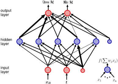
Figure 1: A neural network (multilayer perceptron with 2-5-2 architecture) parametrization of the complex-valued CFF $\mathcal{H}(x_{B},t)$. Each blob symbolizes a neuron and thickness of arrows represents the strengths of weights $w_{j}$. (Smaller blobs with no input are so-called biases — they improve the network’s properties [30].)

Neural networks have been applied to a variety of tasks, including optimization problems. One of the main attractions is their apparent ability to mimic the behavior of human brain: with their multi-connectedness and parallel processing of information they can be trained to perform relatively complex classification and pattern recognition tasks. To this end many kinds of neural networks and corresponding “learning” algorithms have been developed, see, e.g., [30]. In our study, we used one of the most popular neural network types, known as multilayer perceptron. Schematically shown on Fig. 1, it is a mathematical structure consisting of a number of interconnected “neurons” organized in several layers. Each neuron has several inputs and one output. The value at the output is given as a function $f(\sum_{j}w_{j}x_{j})$ of a sum of values at inputs $x_{1},x_{2},\cdots$, each weighted by a a certain number $w_{j}$. Consequently, a multilayer perceptron is defined by its architecture (number of layers and number of neurons in each layer), by the values of its weights, and by the shape of its activation function $f(x)$. Again somewhat inspired by biological neuron properties, the activation function is often taken as a nonlinear function with saturating properties for large and small values of its argument. We employed a very popular logistic sigmoid function

$$f(x)=1/(1+\exp(-x))$$

for neurons in inner (“hidden”) layer(s), while for input and output layers we used the identity function $f(x)=x$. By iterating over the following steps the network is then trained, i.e., it “learns” how to describe a certain set of data points:

1. Kinematic values (two in our case: $x_{B}$ and $t$) of the first data point are presented to two input-layer neurons

2. These values are then propagated through the network according to weights and activation functions. In the first iteration, weights are set to some random value.

3. As a result, the network produces some resulting values of output in its output-layer neurons. Here we have two: $\operatorname{\mathfrak{Im}}\mathcal{H}$ and $\operatorname{\mathfrak{Re}}\mathcal{H}$. Obviously, after the first iteration, these will be some random functions of the input kinematic values: $\operatorname{\mathfrak{Im}}\mathcal{H}(x_{B},t)$ and $\operatorname{\mathfrak{Re}}\mathcal{H}(x_{B},t)$.

4. Using these values of CFF(s), the observable(s) corresponding to the first data point is (are) calculated and it is (they are) compared to actually measured value(s), with squared error used for building the standard $\chi^{2}$ function.

5. The obtained error is then used to modify the network: It is, possibly weighted by the inverse uncertainty of the experimental measurement, propagated backwards through the layers of the network and each weight is adjusted such that this error is decreased. The concrete algorithm for this weight adjustment is discussed at the end of this section.

6. This procedure is then repeated with the next data point, until the whole training set is exhausted.

This sequence of steps (called training epoch) is repeated until the network is capable to describe experimental data with a sufficient accuracy — the precise stopping criterion is specified below.

From what is said it should be clear that a neural network is nothing more but a complicated non-linear multi-parameter function and that the training procedure is equivalent to the least-squares fitting of this function to data. The actual power of the approach stems from the following:

• A neural network serves as unbiased interpolating function. Its complicated dependence on parameters enables it to approximate any smooth function with comparable ease.

• Updating the weights of a given neuron by back-propagation of error uses only values and gradients of activation functions in the immediate network neighborhood. In this sense the training process is local and it is algorithmically efficient.

• This approach enables the following convenient method for propagation of experimental uncertainties (and even their correlations) into the final result: In our application a “replica data set” is interpolated. It is obtained from original data by generating random artificial data points using Gaussian probability distribution with a width defined by the error bar of experimental measurements. Taking a large number $N_{rep}$ of such replicas, the resulting family of trained neural networks $\mathcal{H}^{(1)},\ldots,\mathcal{H}^{(N_{rep})}$ defines a probability distribution of the represented CFF $\mathcal{H}(x_{B},t)$ and of any functional $\mathcal{F}[\mathcal{H}]$ thereof. Thus, the mean value of such a functional and its variance are [31, 18]

  $$\Big{\langle}\mathcal{F}[\mathcal{H}]\Big{\rangle} =\frac{1}{N_{rep}}\sum_{k=1}^{N_{rep}}\mathcal{F}[\mathcal{H}^{(k)}]\;,$$ (4)

  $$\Big{(}\Delta\mathcal{F}[\mathcal{H}]\Big{)}^{2} =\Big{\langle}\mathcal{F}[\mathcal{H}]^{2}\Big{\rangle}-\Big{\langle}\mathcal{F}[\mathcal{H}]\Big{\rangle}^{2}\;.$$ (5)

  For details of this “Monte Carlo” procedure see Refs. [18, 32] and note that this is a general method of error propagation, which is not related to neural networks themselves and can be used also for error propagation in standard least-squares fitting of model functions to data.

The power of neural networks to approximate any continuous function implies also the danger of overfitting the data (also known as overtraining). Namely, after a certain number of iterations the network will not only describe the general dependence of observables on kinematic variables, but will also adjust to the random fluctuations of data. This unwanted behavior is prevented by the cross-validation procedure in which initial data is divided into two sets: training set and validation set. Then performance of the network is continuously checked on the validation set. Since this set is not used for training, after the onset of overfitting, the error of the network’s description of validation sets will increase, see Fig. 2. This is the moment at which training is stopped.

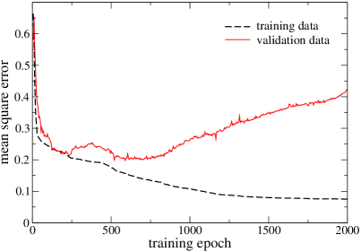
Figure 2: Typical progress of neural network training: the error for the description of training data (dashed) is monotonously decreasing, while the error for the validation data (solid) increases when the neural network is overfitted. In the plotted example one would use the network obtained after 500-700 training epochs as the final result

For more informations on neural networks we refer the reader to the vast literature on the subject, e.g. [30], while the PhD thesis [32] is a good reference for the particular approach used also in this work. In the remainder of this section, we specify some details about the neural networks we used.

In our study we employed the PyBrain software library for neural networks [33]. This choice was motivated by (i) the great flexibility of this library, which allows to explore various types of neural networks, and (ii) it being written in the Python programming language, such that it was easy to link with our already existing Python code for DVCS analysis. Like almost every other freely available neural network software (at least to our knowledge), PyBrain expects that the network output is directly compared to training data samples for error calculation. In our case, however, the network output must be transformed, i.e., the DVCS observables must be calculated from $\operatorname{\mathfrak{Im}}\mathcal{H}$ and $\operatorname{\mathfrak{Re}}\mathcal{H}$ (see step no. 4 in the training procedure described above), before the error can be evaluated. For this, we had to make some modifications to the PyBrain software.

Concerning the network architecture, the number of neurons in the input and output layers were fixed by the problem at hand to be two, see Fig. 1. To fix the number of hidden layers and their neurons, one has to consider a trade-off between two requirements: the number of neurons in the hidden layer(s) must be large enough to ensure sufficient expressive power of the network but must not be too large with respect to the number of available data points, otherwise the training will become difficult. In our case, it is already known from previous studies, e.g. [9], that CFF $\mathcal{H}$ is a reasonably well-behaved function. Thus, since we used a relatively small sample of few tens of data points, see next section, just one hidden layer with about ten neurons proved to be sufficient. The specific results presented in this paper were obtained by training series of neural networks, with 13 neurons in the hidden layer each. We checked that results do not change appreciably if a neuron is added or removed from the hidden layer, which is one of the standard tests in neural network applications.

There are various training algorithms available for updating the network weights, from a simple back-propagation algorithm [30] to genetic algorithms like the one used by the NNPDF group [32, 14]. After some experimentation we ended up using the so called resilient back-propagation algorithm [34]. This algorithm is a modification of the usual back-propagation algorithm: only the signs of the partial derivatives of the error function, and not their magnitude are taken into account. Resilient back-propagation is known to be very reliable, fast and insensitive to parameters of the network and of the learning process. More sophisticated algorithms are needed when correlations are included in the $\chi^{2}$ error function or in cases for which the connection between the network output and the experimental observables is very non-linear. The latter would, e.g. be the case when the network output would represent GPDs rather than CFFs, so that the connection would involve convolutions with QCD evolution operators and hard-scattering coefficient functions. Let us finally note that besides perceptrons, there are attempts to apply other kinds of neural networks in nucleon structure studies, such as self-organizing maps [35].

3 Example fit to data

For the first application, to assess the power of the neural network approach, we took just two sets of measurements of leptoproduction of a real photon by scattering leptons off unpolarized protons. One set consisted of 18 measurements of the first sine harmonic $A_{LU}^{\sin\phi}$ of the beam spin asymmetry (BSA)

$$BSA\equiv\frac{{\rm d}\sigma_{e^{\uparrow}}-{\rm d}\sigma_{e^{\downarrow}}}{{\rm d}\sigma_{e^{\uparrow}}+{\rm d}\sigma_{e^{\downarrow}}}\sim A_{LU}^{\sin\phi}\sin\phi\;,$$ (6)

(where $\phi$ is the azimuthal angle in the so-called Trento convention), while in the other set there were 18 measurements of the first cosine harmonic $A_{C}^{\cos\phi}$ of the beam charge asymmetry (BCA)

$$BCA\equiv\frac{{\rm d}\sigma_{e^{+}}-{\rm d}\sigma_{e^{-}}}{{\rm d}\sigma_{e^{+}}+{\rm d}\sigma_{e^{-}}}\sim A_{C}^{\cos 0\phi}+A_{C}^{\cos\phi}\cos\phi\;.$$ (7)

Both sets cover identical kinematic regions

$$0.05<x_{B}<0.24\,,\quad 0.02<-t/{\rm GeV}^{2}<0.46\,,\quad\mbox{and}\quad 1.2<\mathcal{Q}^{2}/{\rm GeV}^{2}<6.11\,.$$

As mentioned in the Introduction, we assumed that QCD evolution effects can be neglected, i.e., that CFFs are independent of $\mathcal{Q}^{2}$. Furthermore, it has been shown that the hypothesis of CFF $\mathcal{H}$ dominance leads to a successful description of this data [9] and so we relied on this assumption (with the understanding that it is only an approximation which should be given up, once sufficiently precise data is available). Thus, at present, just a single CFF $\mathcal{H}(x_{B},t)$, or two real-valued functions $\operatorname{\mathfrak{Im}}\mathcal{H}(x_{B},t)$ and $\operatorname{\mathfrak{Re}}\mathcal{H}(x_{B},t)$, are extracted from data by our neural networks.

A comment about the relation between $\operatorname{\mathfrak{Im}}\mathcal{H}$ and $\operatorname{\mathfrak{Re}}\mathcal{H}$ is in order. Analytic properties of CFF $\mathcal{H}$ relate these two functions via a “dispersion relation”, which reads in twist-two approximation:

$$\operatorname{\mathfrak{Re}}\mathcal{H}(x^{\prime}_{B}=\frac{2\xi}{1+\xi},t)={\rm PV}\frac{1}{\pi}\int_{0}^{1}\!dx\,\frac{2x}{\xi^{2}-x^{2}}\operatorname{\mathfrak{Im}}\mathcal{H}(x_{B}=\frac{2x}{1+x},t)-{\cal C}(t)\;,$$ (8)

cf. Eqs. (2) and (3). As discussed in the Introduction, this could be used to simplify the fitting function set from

$$\{\operatorname{\mathfrak{Im}}\mathcal{H}(x_{B},t),\operatorname{\mathfrak{Re}}\mathcal{H}(x_{B},t)\}\quad\mbox{to}\quad\{\operatorname{\mathfrak{Im}}\mathcal{H}(x_{B},t),\mathcal{C}(t)\}.$$

However, for two reasons we treat here the imaginary and real part of CFF $\mathcal{H}$ as independent quantities. First, assumption of “dispersion relation” (8) by itself introduces a theoretical bias we want to avoid. In Section 4 we will see that model-dependent least-squares fits that are based on the “dispersion relation” (8) link, e.g., assumptions about the low $x$ behaviour of $\operatorname{\mathfrak{Im}}\mathcal{H}$ to that of $\operatorname{\mathfrak{Re}}\mathcal{H}$ which might lead to rather misleading results. Instead, neural networks which do not make use of (8) give large uncertainties for both, which is probably more realistic.
Second, to implement the “dispersion relation” approach in a neural network framework one would need to either (i) disconnect topologically the network output representing $\mathcal{C}(t)$ from the input representing $x_{B}$, or (ii) to create a separate neural network with one input and one output (1–1) for $\mathcal{C}(t)$ and train it together with the two-inputs-one-output (2–1) network representing $\operatorname{\mathfrak{Im}}\mathcal{H}(x_{B},t)$. Certainly, taking in future all available fixed target data into account, such a strategy might be feasible, and if so, would allow to get rid of the $\mathcal{H}$ dominance hypothesis and might thus improve the phenomenological value of the final result.

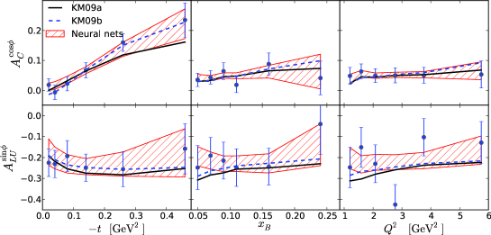
Figure 3: First cosine harmonic of beam charge asymmetry $A_{C}^{\cos\phi}$ (7) and first sine harmonic of beam spin asymmetry $A_{LU}^{\sin\phi}$ (6) resulting from neural network fit (hatched areas), shown together with data [28], used for training. Two model fits, KM09a (solid) and KM09b (dashed) from [9] are also shown for comparison.

Using the procedure described in Section 2, we created 50 replicas from the set of 36 measured data points, which were randomly divided into a training set of 25 points and a validation set of 11 points. Then we trained one neural network on each training set, monitoring progress on the validation set, as in Fig. 2. Training was performed either until the onset of overlearning, or for 2000 epochs, whichever came first. We ended up with 50 neural networks, each representing CFF $\mathcal{H}$. Most of the neural networks fit the original data set quite well (44 of our 50 neural networks have $\chi^{2}$ less than the number of data points, 36), with few poorer fits as expected due to the stochastic nature of the set of data replicas.

Using this set of neural networks as a probability distribution in a functional space of all $\mathcal{H}$ one can predict any function of $\mathcal{H}$, together with its uncertainty, using (4) and (5). As a consistency check we plot in Fig. 3 the result for the very observables that are used for training of networks. We observe that uncertainties of measurements have been correctly propagated into the corresponding uncertainties given by neural networks. This is particularly visible in the first two panels of Fig. 3, where uncertainties of both data and neural networks increase with $|t|$ in the same fashion.

Error bands here and in other figures denote the uncertainty that corresponds to one standard deviation (one sigma). We checked for departures from a Gaussian distribution of network results and found them to be small in the region where data is available. This means that a one-sigma error band corresponds indeed to a 68 % confidence level. However, as observed also by the NNPDF group [14], in the extrapolation region, where there is no data, departures from Gaussian distribution are significant, and 68 % confidence level regions are generally smaller than the one-sigma regions we plot.

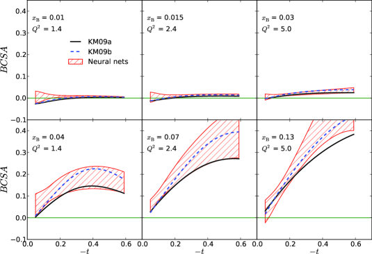
Figure 4: Predictions of neural network fits for beam charge-spin asymmetry (9) in COMPASS II kinematics ($E_{\mu}=160\,{\rm GeV}$, $\phi=0$) (hatched areas). Two model fits, KM09a (solid) and KM09b (dashed) from [9] are also shown for comparison.

As an example of a proper prediction coming from our analysis we plot in Fig. 4 the beam charge-spin asymmetry (BCSA),

$$BCSA\equiv\frac{{\rm d}\sigma_{\mu^{\downarrow+}}-{\rm d}\sigma_{\mu^{\uparrow-}}}{{\rm d}\sigma_{\mu^{\downarrow+}}+{\rm d}\sigma_{\mu^{\uparrow-}}}$$ (9)

as a function of $t$, for several kinematic points that are characteristic for the COMPASS II experiment (where the muon is taken to be massless and the polarization is set equal to 0.8). This experiment was chosen because its kinematics overlaps with that of the HERMES data used for neural network training. Hence these predictions represent partly interpolation and partly extrapolation of HERMES data, thus testing this framework in a nontrivial way.

4 Comparison with model fits and assessment of uncertainties

One of the main advantages of the neural network approach to hadron structure is that it offers a convenient way to assess the uncertainties of non-perturbative functions (GPDs, CFFs, PDFs, …). Let us now emphasize this point further by making a comparison with the common method in which one chooses some model and makes a least-squares fit of it to the data. To quantify this comparison, we took a simple model of the CFF $\mathcal{H}$ and fitted it to the very same data to which neural networks were trained.

We adopted a version of the model used in [9] for which the partonic decomposition of $\operatorname{\mathfrak{Im}}\mathcal{H}$ is:

$$\operatorname{\mathfrak{Im}}{\cal H}(x_{\rm Bj},t)=\pi\left[\left(2\,\frac{4}{9}+\frac{1}{9}\right)H^{\rm val}(\xi,\xi,t)+\frac{2}{9}H^{\rm sea}(\xi,\xi,t)\right]\,.$$ (10)

We parametrized the GPDs along the cross-over trajectory $\xi=x$ as:

$$H(x,x,t)=\frac{n\,r}{1+x}\left(\frac{2x}{1+x}\right)^{-\alpha(t)}\left(\frac{1-x}{1+x}\right)^{b}\frac{1}{\left(1-\frac{1-x}{1+x}\frac{t}{M^{2}}\right)^{p}}\,~{}~{}~{}.$$ (11)

Here $2^{-\alpha(0)}\,n$ is the normalization of PDF $q(x)=H(x,0,0)$ from PDF fits, $r$ is the skewness ratio at small $x$ (the ratio of a GPD at some point on the cross-over trajectory and the corresponding PDF), $\alpha(t)$ is the “Regge trajectory”, $b$ controls the large-$x$ behavior, and $M$ and $p$ control the $t$-dependence [36]. The parameters of the sea-quark GPD $H^{\rm sea}$ were taken to be as in [9] ($\alpha^{\rm sea}(t)=1.13+0.15\,t/{\rm GeV}^{2}$, $n^{\rm sea}=1.35$, $r^{\rm sea}=1$, $b^{\rm sea}=2$, $(M^{\rm sea})^{2}=0.5\,{\rm GeV}^{2}$, $p^{\rm sea}=2$). For the valence quark GPD $H^{\rm val}$, we also fixed $\alpha^{\rm val}(t)=0.43+0.85\,t/{\rm GeV}^{2}$, $n^{\rm val}=1.35$, and $p^{\rm val}=1$. This left $r^{\rm val}$, $b^{\rm val}$ and $M^{\rm val}$ as free parameters, to be determined by the fit to the data. We obtained $\operatorname{\mathfrak{Re}}\mathcal{H}$ from the “dispersion relation” (8), treating the subtraction constant $C$ as a fourth and final free parameter of the model.

Fitting this model to the same 36 data points used for neural network fit, using the well-known Minuit software package [37] for minimization of the $\chi^{2}$ function, resulted in a good fit ($\chi_{0}^{2}/{\rm n.d.o.f}=22.2/32$) with parameter values

$$r^{\rm val}=1.11\,,\quad b^{\rm val}=1.79\,,\quad M^{\rm val}=0.51\,{\rm GeV}\,,\quad C=2.25~{}~{}~{}~{}.$$ (12)

The uncertainty of the resulting fit is commonly determined by the so-called Hessian method. The Hessian matrix is given by the second derivatives of $\chi^{2}$ with respect to the model parameters $a_{i}$ at the minimum $\chi=\chi_{0}$:

$$H_{ij}=\left.\frac{\partial^{2}\chi^{2}}{\partial a_{i}\partial a_{j}}\right|_{\chi=\chi_{0}}\;.$$ (13)

The uncertainty $\Delta f$ of the function $f(a_{i})$ of these parameters, including the uncertainty of the parameters themselves, is given by the error propagation formula

$$(\Delta f)^{2}=\Delta\chi^{2}\sum_{ij}\frac{\partial f}{\partial a_{i}}H^{-1}_{ij}\frac{\partial f}{\partial a_{j}}\;.$$ (14)

In a textbook approach to statistics, one sigma uncertainty is obtained by taking $\Delta\chi^{2}=1$ in this formula. However, there are several problems with this simple procedure. First, $\chi^{2}$ tends to vary very differently in different directions of parameter space, yielding a Hessian with large variations in the eigenvalue spectrum which might then imply numerical difficulties. In our case, where eigenvalues vary over three orders of magnitude, the problem was not so severe. However, in DVCS fits, involving more parameters, we have also observed much stronger variations. To improve the reliability of the Hessian method, we followed an iterative procedure [38] which allows to find natural directions in parameter space and natural step sizes for the finite-difference calculation of the Hessian matrix. Second, it is known that with global fits, i.e., when one combines data from several different experiments, errors are not distributed in the expected way. Often, reasoning strictly within textbook statistics, one would have to reject some data as incompatible either with itself (i.e., because its $\chi^{2}$ is too large) or with other data sets (i.e., because likelihood curves poorly overlap). This is mainly due to systematic errors which are not understood. Without entering further into the discussion of this complex issue, we can follow the CTEQ procedure [39], where $\Delta\chi^{2}$ in (14) is increased ad hoc to $\Delta\chi^{2}=T^{2}$ in order to accommodate all experimental measurements used for fitting. The tolerance parameter $T$ is determined by calculating the average distance from the best fit along eigenvectors of the Hessian matrix at which the model is still compatible with some particular experiment at some confidence level (C.L.). In global PDF fits, with many data sets, values of $T\sim 5-10$ are common, see e.g. [40] for a recent review. Nevertheless, using this procedure, we arrived at a tolerance $T\approx 1$ (for 68 % C.L.; CTEQ use 90 %). We conclude that in our case with just two sets of data, coming from the same experiment, there are no statistical inconsistencies and we can actually use the textbook formula (14) with $\Delta\chi^{2}=1$, which we did. We note in passing that we found that model parameters are significantly more constrained by the BCA than by the BSA data.

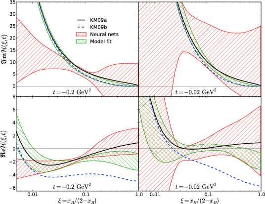
Figure 5: Neural network extraction of $\operatorname{\mathfrak{Im}}{\cal H}(x_{\rm Bj},t)$ and $\operatorname{\mathfrak{Re}}{\cal H}(x_{\rm Bj},t)$ (ascending hatches) from HERMES BCA and BSA [28] data compared with three model fits, one of which with determined uncertainties (descending hatches).

We can now compare the model fit (12), taking also into account uncertainties calculated by the procedure just described, with the neural network parameterization of the CFF $\mathcal{H}$. Both findings are displayed in Fig. 5, together with two models from [9], where $\operatorname{\mathfrak{Im}}\mathcal{H}$ (upper panels) and $\operatorname{\mathfrak{Re}}\mathcal{H}$ (lower panels) are separately plotted. We notice several interesting features:

• In the kinematic region of measured data (this is roughly the middle vertical third of the left panels), there is a good agreement of values and uncertainties of neural networks (ascending hatches) and model fit (descending hatches). This shows that both fitting methods correctly interpolate the data, and that two, quite different, statistical methods used for determination of uncertainties are mutually consistent.

• As one starts to extrapolate the fitted CFF $\cal H$ outside of the data region (left and right thirds of left panels and the whole of the right panels), the two methods predict markedly different shapes and uncertainties for the CFF $\cal H$. All model fits show effects of theoretical bias by following the $x^{-\alpha}$ functional behavior at small $x$ and claiming a small uncertainty there, whereas in neural network parameterizations it is obvious that extrapolated functions are very unconstrained. This is particularly visible in the right panels, illustrating the difficulty of a model-independent extrapolation towards $t=0$, which is a limit of particular interest for hadron structure studies.

• The model fit and the corresponding uncertainties (descending hatches) show the effect of the dispersion relation integral constraint (8) — $\operatorname{\mathfrak{Im}}\mathcal{H}$ is significantly constrained also outside of the data region. This is actually a welcome feature of the dispersion relation fits, offering the opportunity to access nucleon structure in regions not directly accessible in the experiment. However, its usefulness depends on the extent to which the functional forms used are firmly established.

• The model KM09b (dashed line), which was obtained in [9] by including additional data, and, more importantly, by extending the model to include contributions of the CFFs $\widetilde{\mathcal{H}}$ and $\widetilde{\mathcal{E}}$, disagrees for $\operatorname{\mathfrak{Re}}\mathcal{H}$ with the other three fits. This emphasizes that the assumed $\mathcal{H}$ dominance might substantially affect the quality of our results.

5 Conclusions and outlook

Based on HERMES measurements of lepton scattering off unpolarized protons, a reaction which should be dominated by the CFF ${\cal H}$, we performed the first neural network analysis of deeply virtual Compton scattering data and obtained a neural network representation of the CFF $\mathcal{H}$. This was then used to make a prediction for the beam charge-spin asymmetry, measurable at COMPASS II. The Monte Carlo method of propagation of experimental errors enabled us to determine also the uncertainty of the resulting CFF, and we have found that (in the kinematic region where data is available) it agrees well with the uncertainty determined by model fits and standard statistical procedures. However, neural networks combined with Monte Carlo error propagation are a conceptually cleaner and practically simpler method. The propagation of uncertainty from experimental data is intrinsic. Most importantly, this provides essentially a model-independent approach to determine CFFs and GPDs.

One could argue that the neural network approach, just because it is essentially model-independent, does nothing more than faithfully representing the information available in the experimental data by universal objects: CFFs (as presented here) or GPDs (yet to be extracted by this approach). This is valuable in itself but can also be considered as a stepping stone towards improved model-dependent studies, that in principle offer the advantage that our detailed theoretical and phenomenological understanding of QCD dynamics can be taken into account. Such a two-step procedure would be quite natural as models can be more directly compared to neural-network determined CFFs or GPDs than to actual measured observables.

Finally, let us stress that we consider the presented neural network study only as a first step in the analysis of DVCS data. The problem here is that the number of observables measured at a given kinematic point is in practice not sufficient to pin down all twelve CFFs, some of which are kinematically suppressed.

Acknowledgments

K.K. thanks Juan Rojo for many valuable comments and Zvonimir Vlah for discussions on neural networks. D.M. and K.K. are grateful to the Institut für Theoretische Physik, University of Regensburg and to Theory Group of the Nuclear Science Division at Lawrence Berkeley National Laboratory for their warm hospitality. This work was supported by the BMBF grant under the contract no. 06RY9191, by EU FP7 grant HadronPhysics2, by DFG grant, contract no. 436 KRO 113/11/0-1 and by Croatian Ministry of Science, Education and Sport, contract no. 119-0982930-1016.

References

- [1] D. Müller, D. Robaschik, B. Geyer, F. M. Dittes and J. Hořejši, Wave functions, evolution equations and evolution kernels from light-ray operators of QCD, Fortschr. Phys. 42 (1994) 101 [hep-ph/9812448].
- [2] A. V. Radyushkin, Scaling limit of deeply virtual Compton scattering, Phys. Lett. B380 (1996) 417–425 [hep-ph/9604317].
- [3] X.-D. Ji, Deeply-virtual compton scattering, Phys. Rev. D55 (1997) 7114–7125 [hep-ph/9609381].
- [4] X.-D. Ji, Gauge invariant decomposition of nucleon spin, Phys. Rev. Lett. 78 (1997) 610–613 [hep-ph/9603249].
- [5] L. Frankfurt, M. Strikman and C. Weiss, Dijet production as a centrality trigger for collisions at CERN LHC, Phys.Rev. D69 (2004) 114010 [hep-ph/0311231].
- [6] B. Blok, Y. Dokshitzer, L. Frankfurt and M. Strikman, The four jet production at LHC and Tevatron in QCD, Phys. Rev. D83 (2011) 071501 [1009.2714].
- [7] M. Diehl and A. Schäfer, Theoretical considerations on multiparton interactions in QCD, Phys. Lett. B698 (2011) 389–402 [1102.3081].
- [8] S. V. Goloskokov and P. Kroll, The role of the quark and gluon GPDs in hard vector-meson electroproduction, Eur. Phys. J. C53 (2008) 367–384 [0708.3569].
- [9] K. Kumerički and D. Müller, Deeply virtual Compton scattering at small and the access to the GPD H, Nucl. Phys. B841 (2010) 1–58 [0904.0458].
- [10] LHPC Collaboration, J. D. Bratt et. al., Nucleon structure from mixed action calculations using 2+1 flavors of asqtad sea and domain wall valence fermions, Phys. Rev. D82 (2010) 094502 [1001.3620].
- [11] A. V. Belitsky, D. Müller and A. Kirchner, Theory of deeply virtual compton scattering on the nucleon, Nucl. Phys. B629 (2002) 323–392 [hep-ph/0112108].
- [12] A. Belitsky and D. Müller, Exclusive electroproduction revisited: treating kinematical effects, Phys.Rev. D82 (2010) 074010 [1005.5209].
- [13] NNPDF Collaboration, R. D. Ball et. al., A determination of parton distributions with faithful uncertainty estimation, Nucl. Phys. B809 (2009) 1–63 [0808.1231].
- [14] NNPDF Collaboration, R. D. Ball, L. Del Debbio, S. Forte, A. Guffanti, J. I. Latorre et. al., A first unbiased global NLO determination of parton distributions and their uncertainties, Nucl.Phys. B838 (2010) 136–206 [1002.4407].
- [15] R. D. Ball et. al., Impact of Heavy Quark Masses on Parton Distributions and LHC Phenomenology, 1101.1300.
- [16] K. M. Graczyk, P. Plonski and R. Sulej, Neural Network Parameterizations of Electromagnetic Nucleon Form Factors, JHEP 09 (2010) 053 [1006.0342].
- [17] J. Rojo and J. I. Latorre, Neural network parametrization of spectral functions from hadronic tau decays and determination of QCD vacuum condensates, JHEP 0401 (2004) 055 [hep-ph/0401047].
- [18] S. Forte, L. Garrido, J. I. Latorre and A. Piccione, Neural network parametrization of deep-inelastic structure functions, JHEP 05 (2002) 062 [hep-ph/0204232].
- [19] NNPDF Collaboration, L. Del Debbio, S. Forte, J. I. Latorre, A. Piccione and J. Rojo, Unbiased determination of the proton structure function F(2)**p with faithful uncertainty estimation, JHEP 0503 (2005) 080 [hep-ph/0501067].
- [20] O. V. Teryaev, Analytic properties of hard exclusive amplitudes, hep-ph/0510031.
- [21] K. Kumerički, D. Müller and K. Passek-Kumerički, Towards a fitting procedure for deeply virtual Compton scattering at next-to-leading order and beyond, Nucl. Phys. B794 (2008) 244–323 [hep-ph/0703179].
- [22] M. Diehl and D. Y. Ivanov, Dispersion representations for hard exclusive processes, Eur. Phys. J. C52 (2007) 919–932 [0707.0351].
- [23] K. Kumerički, D. Müller and K. Passek-Kumerički, Sum rules and dualities for generalized parton distributions: is there a holographic principle?, Eur. Phys. J. C58 (2008) 193–215 [0805.0152].
- [24] M. Guidal, A fitter code for Deep Virtual Compton Scattering and Generalized Parton Distributions, Eur. Phys. J. A37 (2008) 319–332 [0807.2355].
- [25] M. Guidal and H. Moutarde, Generalized Parton Distributions from Deeply Virtual Compton Scattering at HERMES, Eur. Phys. J. A42 (2009) 71–78 [0905.1220].
- [26] M. Guidal, Generalized Parton Distributions from Deep Virtual Compton Scattering at CLAS, Phys. Lett. B689 (2010) 156–162 [1003.0307].
- [27] H. Moutarde, Extraction of the Compton Form Factor H from DVCS measurements at Jefferson Lab, Phys. Rev. D79 (2009) 094021 [0904.1648].
- [28] HERMES Collaboration, A. Airapetian et. al., Separation of contributions from deeply virtual Compton scattering and its interference with the Bethe–Heitler process in measurements on a hydrogen target, JHEP 11 (2009) 083 [0909.3587].
- [29] COMPASS Collaboration, F. Gautheron et. al., COMPASS-II Proposal, CERN-SPSC-2010-014 (2010) SPSC–P–340. [http://wwwcompass.cern.ch/compass/proposal/compass-II_proposal/compass%-II_proposal.pdf].
- [30] S. Haykin, Neural Networks, A Comprehensive Foundation. Prentice Hall, 2nd ed., 1999.
- [31] W. T. Giele, S. A. Keller and D. A. Kosower, Parton distribution function uncertainties, hep-ph/0104052.
- [32] J. C. Rojo, The Neural network approach to parton distribution functions, hep-ph/0607122. PhD Thesis.
- [33] T. Schaul, J. Bayer, D. Wierstra, Y. Sun, M. Felder, F. Sehnke, T. Rückstieß and J. Schmidhuber, PyBrain, The Journal of Machine Learning Research 11 (2010) 743–746.
- [34] M. Riedmiller, Advanced supervised learning in multi-layer perceptrons, Comput. Standards Interfaces 16 (1994), no. 5 265–278.
- [35] H. Honkanen, S. Liuti, J. Carnahan, Y. Loitiere and P. Reynolds, New avenue to the Parton Distribution Functions: Self-Organizing Maps, Phys.Rev. D79 (2009) 034022 [0810.2598].
- [36] D. S. Hwang and D. Müller, Implication of the overlap representation for modelling generalized parton distributions, Phys. Lett. B660 (2008) 350–359 [0710.1567].
- [37] F. James and M. Roos, Minuit: A system for function minimization and analysis of the parameter errors and correlations, Comput. Phys. Commun. 10 (1975) 343–367.
- [38] J. Pumplin, D. R. Stump and W. K. Tung, Multivariate fitting and the error matrix in global analysis of data, Phys. Rev. D65 (2001) 014011 [hep-ph/0008191].
- [39] J. Pumplin, D. Stump, J. Huston, H. Lai, P. M. Nadolsky et. al., New generation of parton distributions with uncertainties from global QCD analysis, JHEP 0207 (2002) 012 [hep-ph/0201195].
- [40] A. De Roeck and R. Thorne, Structure Functions, 1103.0555.