Shortcuts to adiabaticity for non-Hermitian systems

Abstract

Adiabatic processes driven by non-Hermitian, time-dependent Hamiltonians may be sped up by generalizing inverse engineering techniques based on Berry’s transitionless driving algorithm or on dynamical invariants. We work out the basic theory and examples described by two-level Hamiltonians: the acceleration of rapid adiabatic passage with a decaying excited level and of the dynamics of a classical particle on an expanding harmonic oscillator.

I Introduction

We refer to fast time-dependent processes that reproduce the effect of a slow, adiabatic driving of a quantum system as “shortcuts to adiabaticity” ion ; David ; MN08 ; Muga09 ; S09a ; S09b ; Berry09 ; Salamon09 ; Calarco09 ; Ch10 ; ChenPRL10b ; ChenET10 ; Nice10 ; MN10 ; Muga10 ; Li10 ; Nice11 ; Chen11 ; optimal_control ; Wu11 ; Adol11 ; transport ; transport2 . We also apply the term to the inverse engineering methods used to design these processes. In the adiabatic process of reference the external control parameters are modified slowly from some initial configuration to a final one. In the corresponding shortcut the system is driven in a predetermined short time to a final state which reproduces in the instantaneous basis the initial populations, as the adiabatic process would do, but possibly allowing for some transient excitation along the way. There is nowadays considerable interest in these questions for fundamental and practical reasons. Adiabatic methods are ubiquitous in cold-atom and atomic-physics laboratories to manipulate and prepare atomic states in principle in a robust way. An obvious drawback is that the times required may be too long for practical applications. Moreover the ideal robustness may be spoiled by the accumulation of perturbations and decoherence due to noise and undesired interactions. Studies and experiments to speed up adiabatic processes have been carried out for transport ion ; David ; MN08 ; Calarco09 ; transport ; transport2 , wave splitting S09a ; S09b , expansions and compressions Muga09 ; Salamon09 ; Ch10 ; Muga10 ; ChenET10 ; MN10 ; Nice10 ; Nice11 ; Li10 ; optimal_control ; Wu11 ; Adol11 , or internal state control Berry09 ; ChenPRL10b ; Chen11 . These studies have so far been performed for Hermitian Hamiltonians, but many systems admit an effective non-Hermitian description. In this paper we put forward shortcuts to adiabaticity techniques for non-Hermitian Hamiltonians. Specifically we shall generalize the inverse engineering method proposed by Berry Berry09 and the one based on dynamical invariants Ch10 . While these methods are intimately connected as shown in Chen11 and may in fact be considered potentially equivalent, in standard applications they are used in different ways and provide different answers so we shall consider them separately here. As study cases we shall discuss a two-level decaying atom and the motion of a classical particle in a harmonic oscillator with time-dependent frequency.

I.1 Non-Hermitian Hamiltonians: basic formulae

Non-Hermitian Hamiltonians typically describe subsystems of a larger system Muga04 . We shall first review a basic set of relations and notation Muga04 . We shall assume a non-Hermitian time-dependent Hamiltonian $H_{0}(t)$ with $N$ non-degenerate right eigenstates $\{|n(t)\rangle\}$, $n=1,2...,N$,

$$H_{0}(t)|n(t)\rangle=E_{n}(t)|n(t)\rangle,$$ (1)

and biorthogonal partners $\{|\hat{n}(t)\rangle\}$,

$$H^{{\dagger}}_{0}(t)|\hat{n}(t)\rangle=E_{n}^{*}(t)|\hat{n}(t)\rangle,$$ (2)

where the star means “complex conjugate” and the dagger denotes the adjoint operator. They satisfy

$$\langle\hat{n}(t)|m(t)\rangle=\delta_{nm}$$ (3)

and the closure relations

$$\sum_{n}|\hat{n}(t)\rangle\langle n(t)|=\sum_{n}|n(t)\rangle\langle\hat{n}(t)|=1.$$ (4)

$\langle\hat{n}(t)|$ is the left eigenvector of $H_{0}(t)$,

$$\langle\hat{n}(t)|H_{0}(t)=\langle\hat{n}(t)|E_{n}(t),$$ (5)

and $\langle n(t)|$ the left eigenvector of $H^{{\dagger}}_{0}(t)$,

$$\langle n(t)|H^{{\dagger}}_{0}(t)=\langle n(t)|E_{n}^{*}(t).$$ (6)

We can thus write the Hamiltonian and its adjoint as

$$H_{0}(t) = \sum_{n}|n(t)\rangle E_{n}(t)\langle\hat{n}(t)|,$$

$$H^{{\dagger}}_{0}(t) = \sum_{n}|\hat{n}(t)\rangle E_{n}^{*}(t)\langle n(t)|.$$ (7)

The time-dependent Schrödinger equations for a generic state $|\Psi(t)\rangle$ and for its biorthogonal partner $|\hat{\Psi}(t)\rangle$ satisfying $\langle\hat{\Psi}(t)|\Psi(t)\rangle=1$ are

$$i\hbar\partial_{t}|\Psi(t)\rangle = H_{0}(t)|\Psi(t)\rangle,$$ (8)

$$i\hbar\partial_{t}|\hat{\Psi}(t)\rangle = H^{{\dagger}}_{0}(t)|\hat{\Psi}(t)\rangle.$$ (9)

II Transitionless driving algorithm

In Berry09 M. V. Berry proposed a method to design a Hermitian Hamiltonian $H(t)$ for which the approximate adiabatic dynamics driven by the Hermitian Hamiltonian $H_{0}(t)$ becomes exact. We shall generalize this method for non-Hermitian Hamiltonians. First we need the adiabatic approximation when $H_{0}(t)$ is non-Hermitian adNH1 ; adNH2 . A general time-dependent state $|\Psi(t)\rangle$ is a linear combination of instantaneous eigenvectors $|n(t)\rangle$ of $H_{0}(t)$ with time-dependent coefficients. Similarly $|\hat{\Psi}(t)\rangle$ is a linear combination of instantaneous eigenvectors $|\hat{n}(t)\rangle$ of $H^{\dagger}_{0}(t)$. In the adiabatic approximation we assume that only one of these eigenvectors is populated. To determine the corresponding phase factor we insert

$$|\varphi_{n}(t)\rangle = e^{i\beta_{n}(t)}|n(t)\rangle,$$ (10)

$$|\hat{\varphi}_{n}(t)\rangle = e^{i\hat{\beta}_{n}(t)}|\hat{n}(t)\rangle,$$ (11)

into Eqs. (8) and (9). Thus we have

$$i\dot{\beta}_{n}|n(t)\rangle+|\partial_{t}n(t)\rangle=\frac{H_{0}(t)}{i\hbar}|n(t)\rangle,$$ (12)

$$i\dot{\hat{\beta}}_{n}|\hat{n}(t)\rangle+|\partial_{t}\hat{n}(t)\rangle=\frac{H^{{\dagger}}_{0}(t)}{i\hbar}|\hat{n}(t)\rangle,$$ (13)

where the dot denotes the derivative with respect to time. Multiplying Eq. (12) by $\langle\hat{n}(t)|$ and Eq. (13) by $\langle n(t)|$, taking into account Eqs. (1) and (2), and integrating, we find

$$\beta_{n}(t) = \int^{t}_{0}\left[\frac{-E_{n}(t^{\prime})}{\hbar}+i\langle\hat{n}(t^{\prime})|\partial_{t^{\prime}}n(t^{\prime})\rangle\right]dt^{\prime},$$ (14)

$$\hat{\beta}_{n}(t) = \int^{t}_{0}\left[\frac{-E^{*}_{n}(t^{\prime})}{\hbar}+i\langle n(t^{\prime})|\partial_{t^{\prime}}\hat{n}(t^{\prime})\rangle\right]dt^{\prime},$$ (15)

where the initial phases are set to zero. As $\langle n(t)|\partial_{t}\hat{n}\rangle^{*}=\langle\partial_{t}\hat{n}|n(t)\rangle$ and, from Eq. (3), $\langle\partial_{t}\hat{n}|n(t)\rangle=-\langle\hat{n}(t)|\partial_{t}n\rangle$, we have that $\hat{\beta}_{n}=\beta_{n}^{*}$.

As in Berry09 , we now impose that all $|\varphi_{n}(t)\rangle$ satisfy exactly the Schrödinger equation for a yet unknown $H(t)$,

$$i\hbar\partial_{t}|\varphi_{n}(t)\rangle=H(t)|\varphi_{n}(t)\rangle.$$ (16)

Similarly,

$$i\hbar\partial_{t}|\hat{\varphi}_{n}(t)\rangle=H^{{\dagger}}(t)|\hat{\varphi}_{n}(t)\rangle.$$ (17)

The states $|\varphi_{n}(t)\rangle$ and $|\hat{\varphi}_{n}(t)\rangle$ can be written in terms of the corresponding evolution operators $U(t)$ and $\hat{U}(t)$,

$$|\varphi_{n}(t)\rangle = U(t)|n(0)\rangle,$$

$$|\hat{\varphi}_{n}(t)\rangle = \hat{U}(t)|\hat{n}(0)\rangle.$$ (18)

The Hamiltonian $H(t)$ can be found from

$$i\hbar\partial_{t}U(t)=H(t)U(t),$$ (19)

as

$$H(t)=i\hbar\partial_{t}U(t)\hat{U}^{{\dagger}}(t),$$ (20)

since Muga04

$$\hat{U}^{{\dagger}}(t)U(t)=1_{op}.$$ (21)

The evolution operators can be written as

$$U(t) = \sum_{n}e^{i\beta_{n}(t)}|n(t)\rangle\langle\hat{n}(0)|,$$

$$\hat{U}(t) = \sum_{n}e^{i\hat{\beta}_{n}(t)}|\hat{n}(t)\rangle\langle n(0)|.$$ (22)

Using now Eq. (20),

$$H(t)=H_{0}(t)+H_{1}(t),$$ (23)

where

$$H_{1}(t) = i\hbar\sum_{n}[|\partial_{t}n(t)\rangle\langle\hat{n}(t)|$$ (24)

$$- \langle\hat{n}(t)|\partial_{t}n(t)\rangle|n(t)\rangle\langle\hat{n}(t)|].$$

$H(t)$ drives the system along the adiabatic paths defined by $H_{0}(t)$.

As noted in Berry09 and Chen11 this Hamiltonian is not unique. For a given set $|n(t)\rangle$ the same final populations are found by choosing different phases. Let us rewrite $|\varphi_{n}(t)\rangle$ and $|\hat{\varphi}_{n}(t)\rangle$ in terms of arbitrary phases, $\xi_{n}(t)$ and $\hat{\xi}_{n}(t)$, which we now consider manipulable functions obeying $\xi_{n}(t)=\hat{\xi}_{n}^{*}(t)$ so that $\langle\hat{\varphi}_{n}(t)|\varphi_{n}(t)\rangle=1$,

$$|\varphi_{n}(t)\rangle=e^{i\xi_{n}(t)}|n(t)\rangle,\,\,|\hat{\varphi}_{n}(t)\rangle=e^{i\hat{\xi}_{n}(t)}|\hat{n}(t)\rangle.$$ (25)

We assume $\xi_{n}(0)=\hat{\xi}_{n}(0)=0$ and define the new evolution operators

$$U_{\xi}(t) = \sum_{n}e^{i\xi_{n}(t)}|n(t)\rangle\langle\hat{n}(0)|,$$

$$\hat{U}_{\xi}(t) = \sum_{n}e^{i\hat{\xi}_{n}(t)}|\hat{n}(t)\rangle\langle n(0)|.$$ (26)

From Eq. (20), the corresponding Hamiltonian becomes

$$H_{\xi}(t)=-\hbar\sum_{n}|n(t)\rangle\dot{\xi}_{n}(t)\langle\hat{n}(t)|+i\hbar\sum_{n}|\partial_{t}n(t)\rangle\langle\hat{n}(t)|.$$ (27)

III Transitionless driving algorithm applied to a decaying two-level atom

III.1 $H_{1}(t)$ applied to a decaying two-level atom

As an example of the approach of the previous section we shall speed up adiabatic processes in a two-level atom with spontaneous decay. If the decayed atom escapes from the trap by recoil, a Hamiltonian (rather than master equation) description is enough. We shall also assume a semiclassical treatment of the interaction between a laser electric field linearly polarized in $x$-direction, and a decay rate (inverse life-time) $\Gamma$ from the excited state.

Applying the electric dipole approximation, a laser-adapted interaction picture and the rotating wave approximation, the Hamiltonian is

$$H_{a0}(t)=\frac{\hbar}{2}\left(\begin{array}[]{cc}-\Delta(t)&\Omega_{R}(t)\\ \Omega_{R}(t)&\Delta(t)-i\Gamma\end{array}\right),$$ (28)

in the atomic basis $|1\rangle=\left(\begin{array}[]{rccl}1\\ 0\end{array}\right)$, $|2\rangle=\left(\begin{array}[]{rccl}0\\ 1\end{array}\right)$. The detuning from the atomic transition frequency $\omega_{0}$ is $\Delta(t)=\omega_{0}-\omega_{i}(t)$, where $\omega_{i}(t)$ is the instantaneous field frequency. We assume a slowly varying pulse envelope so that the Rabi frequency $\Omega_{R}(t)$, assumed real, depends on time. In the example below we shall take $\Gamma$ as a constant although, in a general case, it could also depend on time, $\Gamma=\Gamma(t)$, as an effective decay rate controlled by further interactions, see e.g. Zeno . The eigenvalues of this Hamiltonian are

$$E_{\pm}(t)=\frac{\hbar}{4}\left\{-i\Gamma\pm\sqrt{-[\Gamma+2i\Delta(t)]^{2}+4\Omega^{2}_{R}(t)}\right\},$$ (29)

and the normalized eigenstates are

$$|\chi_{+}(t)\rangle=\sin\left(\frac{\alpha}{2}\right)|1\rangle+\cos\left(\frac{\alpha}{2}\right)|2\rangle,$$

$$|\chi_{-}(t)\rangle=\cos\left(\frac{\alpha}{2}\right)|1\rangle-\sin\left(\frac{\alpha}{2}\right)|2\rangle,$$ (30)

where the mixing angle $\alpha=\alpha(t)$ is complex and defined as

$$\tan\alpha=\frac{\Omega_{R}}{\Delta-i\Gamma}.$$ (31)

The adjoint of $H_{a0}(t)$ is

$$H_{a0}^{{\dagger}}(t)=\frac{\hbar}{2}\left(\begin{array}[]{cc}-\Delta(t)&\Omega_{R}(t)\\ \Omega_{R}(t)&\Delta(t)+i\Gamma\end{array}\right),$$ (32)

with eigenvalues $E_{\pm}^{*}(t)$ and normalized eigenstates

$$|\hat{\chi}_{+}(t)\rangle=\sin\left(\frac{\alpha^{*}}{2}\right)|1\rangle+\cos\left(\frac{\alpha^{*}}{2}\right)|2\rangle,$$

$$|\hat{\chi}_{-}(t)\rangle=\cos\left(\frac{\alpha^{*}}{2}\right)|1\rangle-\sin\left(\frac{\alpha^{*}}{2}\right)|2\rangle.$$ (33)

Note that the coefficients are complex conjugate of those in Eq. (30) because $H_{a0}(t)$ is equal to its transpose Muga04 . For this system Eq. (24) takes the form

$$H_{a1}(t) = i\hbar[|\partial_{t}\chi_{+}(t)\rangle\langle\hat{\chi}_{+}(t)|$$ (34)

$$- \langle\hat{\chi}_{+}(t)|\partial_{t}\chi_{+}(t)\rangle|\chi_{+}(t)\rangle\langle\hat{\chi}_{+}(t)|$$

$$+ |\partial_{t}\chi_{-}(t)\rangle\langle\hat{\chi}_{-}(t)|$$

$$- \langle\hat{\chi}_{-}(t)|\partial_{t}\chi_{-}(t)\rangle|\chi_{-}(t)\rangle\langle\hat{\chi}_{-}(t)|],$$

where, according to Eqs. (30) and (33),

$$\langle\hat{\chi}_{\pm}(t)|\partial_{t}\chi_{\pm}(t)\rangle = 0,$$

$$\langle\hat{\chi}_{\mp}(t)|\partial_{t}\chi_{\pm}(t)\rangle = \pm\frac{\dot{\alpha}}{2},$$ (35)

so

$$H_{a1}(t)=\hbar\left(\begin{array}[]{cc}0&C(t)\\ -C(t)&0\end{array}\right),$$ (36)

where $C(t)=i\dot{\alpha}/2$ and

$$\dot{\alpha}=\frac{\dot{\Omega}_{R}[\Delta(t)-i\Gamma/2]-\Omega_{R}(t)(\dot{\Delta}-i\dot{\Gamma}/2)}{[\Delta(t)-i\Gamma/2]^{2}+\Omega^{2}_{R}(t)}.$$ (37)

Then, the Hamiltonian $H_{a}(t)=H_{a0}+H_{a1}$ takes the form

$$H_{a}(t)=\frac{\hbar}{2}\left(\begin{array}[]{cc}-\Delta(t)&\Omega_{R}(t)+2C(t)\\ \Omega_{R}(t)-2C(t)&\Delta(t)-i\Gamma\end{array}\right).$$ (38)

The practical realization of this Hamiltonian is not straightforward. In particular the off-diagonal terms are not the complex conjugate of each other unless the real part of $C(t)$ becomes zero. We shall explore in the following subsection the possibility to manipulate this result by playing with different phases as in Eq. (27).

III.2 $H_{\xi}(t)$ applied to a decaying two-level atom

For the decaying two-level atom, using Eq. (27) with phases $\xi_{+}=\xi_{+}(t)$ and $\xi_{-}=\xi_{-}(t)$ associated with $|\chi_{+}(t)\rangle$ and $|\chi_{-}(t)\rangle$, we find

$$\frac{H_{\xi a}(t)}{\hbar}=$$

$$\!\!\!\!\!\!\left[\!\!\begin{array}[]{cc}-\sin^{2}\!{\left(\frac{\alpha}{2}\right)}\dot{\xi}_{+}-\cos^{2}\!{\left(\frac{\alpha}{2}\right)}\dot{\xi}_{-}\!&\!\frac{\sin{\alpha}}{2}(\dot{\xi}_{-}-\dot{\xi}_{+})+C\\ \frac{\sin{\alpha}}{2}(\dot{\xi}_{-}-\dot{\xi}_{+})-C\!&\!-\cos^{2}\!{\left(\frac{\alpha}{2}\right)}\dot{\xi}_{+}-\sin^{2}\!{\left(\frac{\alpha}{2}\right)}\dot{\xi}_{-}\end{array}\!\!\right]\!\!.$$ (41)

The phases in the matrix elements $H_{\xi a,12}(t)$ and $H_{\xi a,21}(t)$ only affect the first terms, which are equal. In general the manipulation of the phases is not enough to make the non-diagonal terms complex conjugate of each other since this requires not only ${\rm{Im}}[(\dot{\xi}_{-}-\dot{\xi}_{+})\sin\alpha]=0$ but ${\rm{Re}}[C(t)]=0$ too. We also add potentially complex terms in the diagonal that again could complicate the physical realization.

In summary, the phase manipulation does not help to implement the shortcut. In some parameter regimes, however, an approximation to $H_{a1}$ that leads to essentially the same results may be easily realized, as discussed next.

III.3 Forced population inversion

We study now the forced coherent decay from the upper level of a two-level system with slow spontaneous decay. This decay may be driven and accelerated adiabatically with a “rapid” adiabatic passage (RAP) technique, sweeping the laser frequency across resonance. The adjective “rapid” here could be misleading: it simply means “faster than the spontaneous decay” but, as the approach is adiabatic, it fails for short enough times. The adiabaticity criterion is worked out in the appendix. To go beyond the time limits imposed by the breakdown of adiabaticity, shortcut techniques may be applied.

Figure 1: Population of the ground state, $P_{1}(t)$ (solid line), and of the excited state, $P_{2}(t)$ (dashed line), for the Hamiltonian $H_{a0}(t)$. Parameters: $\Gamma=2\pi\times 2$ MHz, $a=(2\pi)^{2}\times 0.01$ GHz², $b=(2\pi)^{2}\times 0.00025$ GHz², and $\Omega_{0}=2\pi\times 100$ MHz.

We consider a linearly chirped Gaussian pulse with detuning $\Delta(t)=\omega_{0}-\omega(t)=-2bt$ and Gaussian Rabi frequency $\Omega_{R}(t)=\Omega_{0}e^{-at^{2}}$.

The initial conditions are $P_{1}(0)=0$ and $P_{2}(0)=1$. In Fig. 1 we show that the application of a RAP pulse with $H_{a0}(t)$ is only partially successful. Note the slow spontaneous decay before and after the pulse, and a faster forced transition during the pulse around $t=0$. Since the pulse duration is too short, adiabaticity fails. Fig. 2 shows the fast full population inversion when adding the Hamiltonian $H_{a1}(t)$ in Eq. (36). This Hamiltonian has off-diagonal terms with real and imaginary parts depicted in Fig. 3. Whereas the imaginary parts, the bigger bumps in Fig. 3, are realizable ChenPRL10b , the real parts constitute a non-Hermitian contribution. They are however small, and an approximation of $H_{a1}(t)$ neglecting them provides essentially the same dynamics, as shown in Fig. 2. This remains valid in the strong-driving regime in which $\Gamma\ll\Omega_{0}$ and the natural lifetime is large compared to the duration of the forced decay.

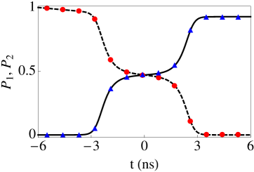
Figure 2: (Color online) Population of the ground state, $P_{1}(t)$ (solid line), and of the excited state, $P_{2}(t)$ (dashed line), for the total Hamiltonian $H_{a}(t)$, coinciding with the populations $P_{1}(t)$ (triangles) and $P_{2}(t)$ (circles) when $H_{a}(t)$ is approximated by neglecting ${\rm{Re}}[C(t)]$. Parameters as in Fig. 1.

Figure 3: Real (solid line) and imaginary (dashed line) parts of $C$. Parameters as in Fig. 1.

IV Invariants based inverse engineering

Lewis and Riesenfeld LR proposed the use of dynamical invariants of a quantum mechanical system to perform expansions of arbitrary time-dependent wave functions by superposition of eigenstates of the invariant. This may be generalized to non-Hermitian Hamiltonians Gao91 ; Gao92 ; Gao93 . We shall assume that for a Hamiltonian $H_{0}(t)$ with the features described in Sec. I.1, there is a generalized invariant $I(t)$ that satisfies

$$\frac{\partial{I}(t)}{\partial{t}}-{\frac{i}{\hbar}}[I(t),H_{0}(t)]=0,$$ (43)

so that $\frac{d}{dt}\langle\hat{\Psi}(t)|I(t)|\Psi(t)\rangle=0$. Note that this is not an ordinary expectation value $\langle\Psi(t)|I(t)|\Psi(t)\rangle/\langle\Psi(t)|\Psi(t)\rangle$, in this sense the concept of generalized invariant differs from the one for Hermitian Hamiltonians.

Let us assume also that $I(t)$ has a non-degenerate complete biorthonormal set of instantaneous eigenstates, $\{|\psi_{n}(t)\rangle,|\hat{\psi}_{n}(t)\rangle\}$, where $n$ varies from $1$ to $N$, that satisfy

$$I(t)|\psi_{n}(t)\rangle = I_{n}(t)|\psi_{n}(t)\rangle,$$ (44)

$$I^{{\dagger}}(t)|\hat{\psi}_{n}(t)\rangle = I_{n}^{*}(t)|\hat{\psi}_{n}(t)\rangle,$$ (45)

$$\langle\hat{\psi}_{m}(t)|\psi_{n}(t)\rangle = \delta_{mn},$$ (46)

$$\sum_{n}|\hat{\psi}_{n}(t)\rangle\langle\psi_{n}(t)| = 1.$$ (47)

We can write the general solutions of the Schrödinger equations for $H_{0}(t)$ and $H_{0}^{{\dagger}}(t)$, Eqs. (8) and (9), as

$$|\Psi(t)\rangle = \sum_{n}d_{n}e^{i\alpha_{n}(t)}|\psi_{n}(t)\rangle,$$ (48)

$$|\hat{\Psi}(t)\rangle = \sum_{n}\hat{d}_{n}e^{i\alpha_{n}^{*}(t)}|\hat{\psi}_{n}(t)\rangle,$$ (49)

where the coefficients $\{d_{n}\}$ and $\{\hat{d}_{n}\}$ do not depend on time, and the generalized Lewis-Riesenfeld phases are

$$\alpha_{n}(t)=\int_{0}^{t}\bigg{\langle}\hat{\psi}_{n}(t^{\prime})\bigg{|}i\frac{\partial}{\partial{t^{\prime}}}-H(t^{\prime})\bigg{|}\psi_{n}(t^{\prime})\bigg{\rangle}dt^{\prime}.$$ (50)

Inverse engineering techniques rely on designing the invariant eigenvectors and phase factors first, possibly taking into account partial information on the structure of the Hamiltonian, and then deducing the Hamiltonian from them.

V Classical particle in an expanding harmonic trap

It is possible to study a classical particle with position $q(t)$ and momentum $p(t)$ in a harmonic trap as a formal quantum two-level system with non-Hermitian Hamiltonian, by rewriting the classical canonical equations of motion in matrix form Gao91 ; Gao92 . The Hamiltonian of a classical harmonic oscillator with a time dependent frequency $\omega(t)$ is

$$H_{ho}(t)=\frac{p^{2}}{2m}+\frac{1}{2}m\omega^{2}(t)q^{2},$$ (51)

where $m$ is the mass of the particle. We shall consider an expansion from $\omega_{0}=\omega(0)$ at $t=0$ to $\omega_{f}=\omega(t_{f})$ at the final time $t=t_{f}$, with $\omega_{f}<\omega_{0}$. The corresponding classical canonical equations

$$\dot{q}_{j} = \frac{\partial{H_{ho}}}{\partial{p}_{j}}=\frac{p(t)}{m},$$ (52)

$$\dot{p}_{j} = -\frac{\partial{H_{ho}}}{\partial{q}_{j}}=-m\omega^{2}(t)q(t),$$ (53)

can be written as

$$\left(\begin{array}[]{cc}\dot{q}\\ \dot{p}\end{array}\right)=\left(\begin{array}[]{cc}0&1/m\\ -m\omega^{2}(t)&0\end{array}\right)\left(\begin{array}[]{cc}q(t)\\ p(t)\end{array}\right),$$ (54)

due to their linear dependence on $q$ and $p$. Multiplying both sides of the equality by $i$ we obtain a Schrödinger-like equation ($\hbar=1$) with the “effective” non-Hermitian Hamiltonian

$$\mathcal{H}(t)=i\left(\begin{array}[]{cc}0&1/m\\ -m\omega^{2}(t)&0\end{array}\right).$$ (55)

This is a useful but formal analogy, since this Hamiltonian does not have units of energy, in fact different matrix elements have different units as the “state vector” components $q$ and $p$ have also different units. Nevertheless we may apply the generalized invariant theory, and expand the state vector in terms of formal eigenvectors of the generalized invariants. Defining Gao92

$$\mathcal{I}(t)=\left(\begin{array}[]{cc}b(t)&c(t)\\ -a(t)&-b(t)\end{array}\right),$$ (56)

and imposing Eq. (43), without $\hbar$,

$$a(t) = m\left[\frac{\omega_{0}}{\varrho^{2}(t)}+\frac{1}{\omega_{0}}\dot{\varrho}^{2}(t)\right],$$ (57)

$$b(t) = \frac{-1}{\omega_{0}}\varrho(t)\dot{\varrho}(t),$$ (58)

$$c(t) = \frac{\varrho^{2}(t)}{\omega_{0}m},$$ (59)

where the dimensionless scaling function $\varrho(t)$ satisfies the auxiliary equation

$$\ddot{\varrho}(t)+\omega^{2}(t)\varrho(t)=\frac{\omega^{2}_{0}}{\varrho^{3}(t)},$$ (60)

which is the Ermakov equation, the same equation for the scaling function that defines the invariants in the expansion of the quantum harmonic oscillator Ch10 . For $\mathcal{I}(t)$, whose eigenvalues are $I_{\pm}=\mp i$, the eigenstates are

$$|\psi_{\pm}(t)\rangle=\left(\begin{array}[]{cc}c(t)\\ \pm i\left[1\pm ib(t)\right]\end{array}\right),$$ (61)

in the basis used in Eq. (55). The Lewis-Riesenfeld phases $\alpha_{\pm}(t)$ are

$$\alpha_{\pm}(t) = \int_{0}^{t}\bigg{\langle}\hat{\psi}_{\pm}(t^{\prime})\bigg{|}i\frac{\partial}{\partial{t^{\prime}}}-\mathcal{H}(t^{\prime})\bigg{|}\psi_{\pm}(t^{\prime})\bigg{\rangle}dt^{\prime}$$ (62)

$$= i\ln{\sqrt{\frac{c(t)}{c(0)}}}\pm\omega_{0}\int_{0}^{t}\frac{1}{\varrho^{2}(t^{\prime})}dt^{\prime}.$$

Then, the phase-space trajectory is given by

$$\left(\begin{array}[]{cc}q(t)\\ p(t)\end{array}\right) = d_{+}e^{i\alpha_{+}(t)}|\psi_{+}(t)\rangle+d_{-}e^{i\alpha_{-}(t)}|\psi_{-}(t)\rangle$$ (65)

$$= \!R\!\left(\!\!\begin{array}[]{cc}\varrho(t)\cos{\theta(t)}\\ -\frac{m\omega_{0}}{\varrho(t)}\sin{\theta(t)}+m\dot{\varrho}(t)\cos{\theta(t)}\end{array}\!\!\right)\!,$$ (68)

where $R=2r\sqrt{c(0)/m\omega_{0}}$ is a distance, $d_{+}=d_{-}^{*}=r\exp{(i\theta_{0})}$ can be determined by the initial conditions at $t=0$, and

$$\theta(t)=\omega_{0}\int_{0}^{t}\frac{1}{\varrho^{2}(t^{\prime})}dt^{\prime}+\theta_{0},$$ (69)

with $\theta_{0}$ the initial phase.

Imposing the boundary conditions $\varrho(0)=1$ and $\dot{\varrho}(0)=0$, and $\varrho(t_{f})=(\omega_{0}/\omega_{f})^{1/2}$ and $\dot{\varrho}(t_{f})=0$, which consistently with the Ermakov equation imply $\ddot{\varrho}(0)=\ddot{\varrho}(t_{f})=0$, we find $E_{0}:=E(t=0)=\omega_{0}^{2}R^{2}m/2$ and $E_{f}:=E(t_{f})=\omega_{f}E_{0}/\omega_{0}$. In other words, these boundary conditions guarantee that the value of the classical adiabatic invariant $E(t)/\omega(t)$ at initial and final times coincides, even though it may take different values at intermediate times.

To design the process, $\varrho(t)$ has to be interpolated at intermediate times. We assume here a polynomial form, $\varrho(t)=\sum_{n=0}^{5}a_{n}t^{n}$, where the coefficients $a_{n}$ are fixed from the boundary conditions. Then we get $\omega(t)$ from the Ermakov equation,

$$\omega(t)=\sqrt{\frac{\omega_{0}^{2}}{\varrho^{4}(t)}-\frac{\ddot{\varrho}(t)}{\varrho(t)}}.$$ (70)

In Fig. 4 we have represented the shortcut trajectory in phase space between the initial and final times, $t=0$ and $t=t_{f}$, for the frequency $\omega(t)$ given by Eq. (70). We have also added a period $T_{0}=2\pi/\omega_{0}$ before $t=0$, and a period $T_{f}=2\pi/\omega_{f}$ after $t=t_{f}$, for which the particle evolves for fixed $\omega_{0}$ and $\omega_{f}$, respectively, so as to depict complete initial and final ellipses. The shortcut trajectory that connects the initial and final ellipses is clearly not an adiabatic path, that would be formed by a succession of slowly varying ellipses from the initial to the final one.

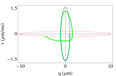
Figure 4: (Color online) Parametric velocity-position trajectory. The initial ellipse (solid blue thin line) and the final ellipse (red dashed line) are connected by the shortcut trajectory (green solid thick line). Parameters: $\theta_{0}=0$ corresponding to $q_{0}=q(t=0)=1$ $\mu$m and $v_{0}=v(t=0)=0$ $\mu$m/ms, $\omega_{0}=2\pi\times 250$ Hz, $\omega_{f}=2\pi\times 2.5$ Hz, $t_{f}=25$ ms, and the mass of an atom of Rubidium-87, $m=1.44\times 10^{-25}$ kg.

VI Discussion and Conclusion

We have generalized shortcut to adiabaticity techniques for non-Hermitian Hamiltonian systems and provided application examples. Experimental implementations are at reach. Related open questions are the application of similar concepts to master equations, or developing means to implement arbitrary non-Hermitian interactions. Another interesting research avenue is to combine shortcut techniques with optimal control Li10 ; optimal_control taking into account physically imposed constraints.

Appendix A Adiabaticity condition for time-dependent non-Hermitian Hamiltonians applied to a decaying two-level atom

The adiabaticity condition for time-dependent Hermitian Hamiltonians is given by

$$|\langle n(t)|\partial_{t}m(t)\rangle|\ll\frac{1}{\hbar}|E_{n}(t)-E_{m}(t)|,\;n\neq m,$$ (71)

in terms of instantaneous eigenstates and eigenvalues. Following closely its derivation in Schiff we generalize it for non-Hermitian Hamiltonians as

$$|\langle\hat{n}(t)|\partial_{t}{m}(t)\rangle|\ll\frac{1}{\hbar}|E_{n}(t)-E_{m}(t)|.$$ (72)

For the two-level decaying atom this condition is

$$|\langle\hat{n}_{+}(t)|\partial_{t}{n}_{-}(t)\rangle|\ll\frac{1}{\hbar}|E_{+}(t)-E_{-}(t)|.$$ (73)

Introducing here Eqs. (29), (30) and (33), the adiabaticity condition for this system takes the form

$$2|\Omega_{a}(t)|\ll|\Omega(t)|,$$ (74)

where $\Omega(t)=\sqrt{-[\Gamma+2i\Delta(t)]^{2}+4\Omega^{2}_{R}(t)}$ and $\Omega_{a}(t)=-\dot{\alpha}/2$.

References

- (1) R. Reichle, D. Leibfried, R. B. Blakestad, J. Britton, J. D. Jost, E. Knill, C. Langer, R. Ozeri, S. Seidelin, and D. J. Wineland, Fortschr. Phys. 54, 666 (2006).
- (2) A. Couvert, T. Kawalec, G. Reinaudi, and D. Guéry-Odelin, Europhys. Lett. 83, 13001 (2008).
- (3) S. Masuda and K. Nakamura, Phys. Rev. A 78, 062108 (2008).
- (4) M. Murphy, L. Jiang, N. Khaneja, and T. Calarco, Phys. Rev. A 79, 020301(R) (2009).
- (5) E. Torrontegui, S. Ibáñez, X. Chen, A. Ruschhaupt, D. Guéry-Odelin, and J. G. Muga, Phys. Rev. A 83, 013415 (2011).
- (6) E. Torrontegui, X. Chen, M. Modugno, S. Schmidt, A. Ruschhaupt, and J. G. Muga, arXiv:1103.2532.
- (7) J. Grond, J. Schmiedmayer, and U. Hohenester, Phys. Rev. A 79, 021603 (2009).
- (8) J. Grond, G. von Winckel, J. Schmiedmayer, and U. Hohenester, Phys. Rev. A 80, 053625 (2009).
- (9) J. G. Muga, X. Chen, A. Ruschhaupt, and D. Guéry-Odelin, J. Phys. B 42, 241001 (2009).
- (10) P. Salamon, K. H. Hoffmann, Y. Rezek, and R. Kosloff, Phys. Chem. Chem. Phys. 11, 1027 (2009).
- (11) X. Chen, A. Ruschhaupt, S. Schmidt, A. del Campo, D. Guéry-Odelin, and J. G. Muga, Phys. Rev. Lett. 104, 063002 (2010).
- (12) X. Chen and J. G. Muga, Phys. Rev. A 82, 053403 (2010).
- (13) J. F. Schaff, X. L. Song, P. Vignolo, and G. Labeyrie, Phys. Rev. A 82, 033430 (2010).
- (14) S. Masuda and K. Nakamura, Proc. R. Soc. A 466, 1135 (2010).
- (15) J. G. Muga, X. Chen, S. Ibáñez, I. Lizuain, and A. Ruschhaupt, J. Phys. B 43, 085509 (2010).
- (16) D. Stefanatos, J. Ruths, and Jr-Shin Li, Phys. Rev. A 82, 063422 (2010).
- (17) J. F. Schaff, X. L. Song, P. Capuzzi, P. Vignolo, and G. Labeyrie, Europhys. Lett. 93, 23001 (2011).
- (18) Y. Li, L.-A. Wu, and Z.-D. Wang, Phys. Rev. A 83, 043804 (2011).
- (19) A. del Campo, arXiv:1103.0714.
- (20) B. Andresen, K. H. Hoffmann, J. Nulton, A. Tsirlin, and P. Salamon, Eur. J. Phys. 32, 827 (2011).
- (21) M. V. Berry, J. Phys. A 42, 365303 (2009).
- (22) X. Chen, I. Lizuain, A. Ruschhaupt, D. Guéry-Odelin, and J. G. Muga, Phys. Rev. Lett. 105, 123003 (2010).
- (23) X. Chen, E. Torrontegui, and J. G. Muga, (2011) arXiv: 1102.3449v1, accepted in Phys. Rev. A.
- (24) J. G. Muga, J. P. Palao, B. Navarro, and I. L. Egusquiza, Phys. Rep. 395, 357 (2004).
- (25) J. C. Garrison and E. M. Wright, Phys. Lett. A 128, 177 (1988).
- (26) A. Mostafazadeh, J. Math. Phys. 40, 3311 (1999).
- (27) J. G. Muga, J. Echanobe, A. del Campo, and I Lizuain, J. Phys. B: At. Mol. Opt. Phys. 41, 175501 (2008).
- (28) H. R. Lewis and W. B. Riesenfeld, J. Math. Phys. 10, 1458 (1969).
- (29) X. C. Gao, J. B. Xu, and T. Z. Qian, Phys. Rev. A 44, 7016 (1991).
- (30) X. C. Gao, J. B. Xu, and T. Z. Qian, Phys. Rev. A 46, 3626 (1992).
- (31) T. Z Qian, X. C. Gao, and J. B. Xu, Phys. Rev. A 48, 11401 (1993).
- (32) L. I. Schiff, Quantum Mechanics (McGraw-Hill, New York, 1981).