Orthogonal Matching Pursuit with Replacement

Abstract

In this paper, we consider the problem of compressed sensing where the goal is to recover almost all the sparse vectors using a small number of fixed linear measurements. For this problem, we propose a novel partial hard-thresholding operator that leads to a general family of iterative algorithms. While one extreme of the family yields well known hard thresholding algorithms like ITI and HTPMalekiD10 ; Foucart10 , the other end of the spectrum leads to a novel algorithm that we call Orthogonal Matching Pursuit with Replacement (OMPR). OMPR, like the classic greedy algorithm OMP, adds exactly one coordinate to the support at each iteration, based on the correlation with the current residual. However, unlike OMP, OMPR also removes one coordinate from the support. This simple change allows us to prove that OMPR has the best known guarantees for sparse recovery in terms of the Restricted Isometry Property (a condition on the measurement matrix). In contrast, OMP is known to have very weak performance guarantees under RIP. Given its simple structure, we are able to extend OMPR using locality sensitive hashing to get OMPR-Hash, the first provably sub-linear (in dimensionality) algorithm for sparse recovery. Our proof techniques are novel and flexible enough to also permit the tightest known analysis of popular iterative algorithms such as CoSaMP and Subspace Pursuit. We provide experimental results on large problems providing recovery for vectors of size up to million dimensions. We demonstrate that for large-scale problems our proposed methods are more robust and faster than existing methods.

1 Introduction

We nowadays routinely face high-dimensional datasets in diverse application areas such as biology, astronomy, finance and the web. The associated curse of dimensionality is often alleviated by prior knowledge that the object being estimated has some structure. One of the most natural and well-studied structural assumption for vectors is sparsity. Accordingly, a huge amount of recent work in machine learning, statistics and signal processing has been devoted to finding better ways to leverage sparse structures. Compressed sensing, a new and active branch of modern signal processing, deals with the problem of designing measurement matrices and recovery algorithms, such that almost all sparse signals can be recovered from a small number of measurements. It has important applications in imaging, computer vision and machine learning (see, for example, DuarteDTLSKB08 ; WrightMMSHY10 ; HsuKLZ10 ).

In this paper, we focus on the compressed sensing setting (CandesT05, ; Donoho06, ) where we want to design a measurement matrix $A\in\mathbb{R}^{m\times n}$ such that a sparse vector $x^{\star}\in\mathbb{R}^{n}$ with $\|x^{\star}\|_{0}:=|\operatorname{supp}(x^{\star})|\leq k<n$ can be efficiently recovered from the measurements $b=Ax^{\star}\in\mathbb{R}^{m}$. Initial work focused on various random ensembles of matrices $A$ such that, if $A$ was chosen randomly from that ensemble, one would be able to recover all or almost all sparse vectors $x^{\star}$ from $Ax^{\star}$. CandesT05 isolated a key property called the restricted Isometry property (RIP) and proved that, as long as the measurement matrix $A$ satisfies RIP, the true sparse vector can be obtained by solving an $\ell_{1}$-optimization problem,

$$\min\ \|x\|_{1}\text{ s.t. }Ax=b\ .$$

The above problem can be easily formulated as a linear program and is hence efficiently solvable. We recall for the reader that a matrix $A$ is said to satisfy RIP of order $k$ if there is some $\delta_{k}\in[0,1)$ such that, for all $x$ with $\|x\|_{0}\leq k$, we have

$$(1-\delta_{k})\|x\|^{2}\leq\|Ax\|^{2}\leq(1+\delta_{k})\|x\|^{2}\ .$$

Several random matrix ensembles are known to satisfy $\delta_{ck}<\theta$ with high probability provided one chooses $m=O\left(\frac{ck}{\theta^{2}}\log\frac{n}{k}\right)$ measurements. Candes08 showed that $\ell_{1}$-minimization recovers all $k$-sparse vectors provided $A$ satisfies $\delta_{2k}<0.414$ although the condition has been recently improved to $\delta_{2k}<0.473$ (Foucart10b, ). Note that, in compressed sensing, the goal is to recover all, or most, $k$-sparse signals using the same measurement matrix $A$. Hence, weaker conditions such as restricted convexity NRWY09 studied in the statistical literature (where the aim is to recover a single sparse vector from noisy linear measurements) typically do not suffice. In fact, if RIP is not satisfied then multiple sparse vectors $x$ can lead to the same observation $b$, hence making recovery of the true sparse vector impossible.

Based on its RIP guarantees, $\ell_{1}$-minimization can guarantee recovery using just $O(k\log(n/k))$ measurements, but it has been observed in practice that $\ell_{1}$-minimization is too expensive in large scale applications (DonohoMaMo09, ), for example, when the dimensionality is in the millions. This has sparked a huge interest in iterative methods for sparse recovery. An early classic iterative method is Orthogonal Matching Pursuit (OMP) (PatiRK93, ; DavidMA97, ) that greedily chooses elements to add to the support. It is a natural, easy-to-implement and fast method but unfortunately lacks strong theoretical guarantees. Indeed, it is known that, if run for $k$ iterations, OMP cannot uniformly recover all $k$-sparse vectors under an RIP condition of the form $\delta_{2k}\leq\theta$ (Rauhut08, ; MoS11, ). However, Zhang10 showed that OMP, if run for $30k$ iterations, recovers the optimal solution for $\delta_{31k}\leq 1/3$; a significantly more restrictive condition than the ones required by other methods like $\ell_{1}$-minimization.

Several other iterative approaches have been proposed that include Iterative Soft Thresholding (IST) (MalekiD10, ), Iterative Hard Thresholding (IHT) (BlumensathD09, ), Compressive Sampling Matching Pursuit (CoSaMP) (NeedellT09, ), Subspace Pursuit (SP) (DaiM09, ), Iterative Thresholding with Inversion (ITI) (Maleki09, ), Hard Thresholding Pursuit (HTP) (Foucart10, ) and many others. Among the family of iterative hard thresholding algorithms, following MalekiD10 , we can identify two major subfamilies: one- and two-stage algorithms. As their names suggest, the distinction is based on the number of stages in each iteration of the algorithm. One-stage algorithms such as IHT, ITI and HTP, decide on the choice of the next support set and then usually solve a least squares problem on the updated support. The one-stage methods always set the support set to have size $k$, where $k$ is the target sparsity level. On the other hand, two-stage algorithms, notable examples being CoSaMP and SP, first enlarge the support set, solve a least squares on it, and then reduce the support set back again to the desired size. A second least squares problem is then solved on the reduced support. These algorithms typically enlarge and reduce the support set by $k$ or $2k$ elements. An exception is the two-stage algorithm FoBa Zhang08 that adds and removes single elements from the support. However, it differs from our proposed methods as its analysis requires very restrictive RIP conditions ($\delta_{8k}<0.1$ as quoted in HsuKLZ10 ) and the connection to locality sensitive hashing (see below) is not made. Another algorithm with replacement steps appears in ShwartzSZ10 . However, the algorithm and the setting under which it is analyzed are different from ours.

In this paper, we present, and provide a unified analysis for a family of one-stage iterative hard thresholding algorithms. The family is parameterized by a positive integer $l\leq k$. At the extreme value $l=k$, we recover the algorithm ITI/HTP. At the other extreme $k=1$, we get a novel algorithm that we call Orthogonal Matching Pursuit with Replacement (OMPR). OMPR can be thought of as a simple modification of the classic greedy algorithm OMP: instead of simply adding an element to the existing support, it replaces an existing support element with a new one. Surprisingly, this change allows us to prove sparse recovery under the condition $\delta_{2k}<0.499$. This is the best $\delta_{2k}$ based RIP condition under which any method, including $\ell_{1}$-minimization, can be shown to provably perform sparse recovery.

OMPR also lends itself to a faster implementation using locality sensitive hashing (LSH). This allows us to provide recovery guarantees using an algorithm whose run-time is provably sub-linear in $n$, the number of dimensions. An added advantage of OMPR, unlike many iterative methods, is that no careful tuning of the step-size parameter is required even under noisy settings or even when RIP does not hold. The default step-size of $1$ is always guaranteed to converge to at least a local optima.

Finally, we show that our proof techniques used in the analysis of the OMPR family are useful in tightening the analysis of two-stage algorithms, such as CoSaMP and SP, as well. As a result, we are able to prove better recovery guarantees for these algorithms — $\delta_{4k}<0.35$ for CoSaMP and $\delta_{3k}<0.35$ for SP. We hope that this unified analysis sheds more light on the interrelationships between the various kinds of iterative hard thresholding algorithms.

In summary, the contributions of this paper are as follows.

• We present a family of iterative hard thresholding algorithms that on one end of the spectrum includes existing algorithms such as ITI/HTP while on the other end gives OMPR. OMPR is an improvement over the classical OMP method as it enjoys better theoretical guarantees and is also better practically as shown in our experiments.

• Unlike other improvements over OMP, such as CoSaMP or SP, OMPR changes only one element of the support at a time. This allows us to use Locality Sensitive Hashing (LSH) to speed it up resulting in the first provably sub-linear (in the ambient dimensionality $n$) time sparse recovery algorithm.

• We provide a general proof for all the algorithms in our partial hard thresholding based family. In particular, we can guarantee recovery using OMPR, under both noiseless and noisy settings, provided $\delta_{2k}<0.499$. This is the least restrictive $\delta_{2k}$ condition under which any efficient sparse recovery method is known to work. Furthermore, our proof technique can be used to provide a general theorem that provides the least restrictive known guarantees for all the two-stage algorithms such as CoSamp and SP (see Appendix D).

All proofs omitted from the main body of the paper can be found in the appendix.

2 Orthogonal Matching Pursuit with Replacement

Orthogonal matching pursuit (OMP), is a classic iterative algorithm for sparse recovery. At every stage, it selects a coordinate to include in the current support set by maximizing the inner product between columns of the measurement matrix $A$ and the current residual $b-Ax^{t}$. Once the new coordinate has been added, it solves a least squares problem to fully minimize the error on the current support set. As a result, the residual becomes orthogonal to the columns of $A$ that correspond to the current support set. Thus, the least squares step is also referred to as orthogonalization by some authors (DavenportW10, ).

Let us briefly explain some of our notation. We use the MATLAB notation:

$$A\backslash b:=\operatorname*{argmin}_{x}\|Ax-b\|_{2}\ .$$

The hard thresholding operator $H_{k}(\cdot)$ sorts its argument vector in decreasing order (in absolute value) and retains only the top $k$ entries. It is defined formally in the next section. Also, we use subscripts to denote sub-vectors and submatrices, e.g. if $I\subseteq[n]$ is a set of cardinality $k$ and $x\in\mathbb{R}^{n}$, $x_{I}\in\mathbb{R}^{k}$ denotes the sub-vector of $x$ indexed by $I$. Similarly, $A_{I}$ for a matrix $A\in\mathbb{R}^{m\times n}$ denotes a sub-matrix of size $m\times k$ with columns indexed by $I$. The complement of set $I$ is denoted by $\bar{I}$ and $x_{\bar{I}}$ denotes the subvector not indexed by $I$. The support (indices of non-zero entries) of a vector $x$ is denoted by $\operatorname{supp}(x)$.

Our new algorithm called Orthogonal Matching Pursuit with Replacement (OMPR ), shown as Algorithm 1, differs from OMP in two respects. First, the selection of the coordinate to include is based not just on the magnitude of entries in $A^{T}(b-Ax^{t})$ but instead on a weighted combination $x^{t}+\eta A^{T}(b-Ax^{t})$ with the step-size $\eta$ controlling the relative importance of the two addends. Second, the selected coordinate replaces one of the existing elements in the support, namely the one corresponding to the minimum magnitude entry in the weighted combination mentioned above.

Once the support ${I_{t+1}}$ of the next iterate has been determined, the actual iterate $x^{t+1}$ is obtained by solving the least squares problem:

$$x^{t+1}=\operatorname*{argmin}_{x\>:\>\operatorname{supp}(x)={I_{t+1}}}\ \|Ax-b\|_{2}\ .$$

Note that if the matrix $A$ satisfies RIP of order $k$ or larger, the above problem will be well conditioned and can be solved quickly and reliably using an iterative least squares solver.

Algorithm 1 OMPR

1:  Input: matrix $A$, vector $b$, sparsity level $k$

2:  Parameter: step size $\eta>0$

3:  Initialize $x^{1}$ s.t. $|\operatorname{supp}(x^{1})|=k$

4:  for $t=1$ to $T$ do

5:     $z^{t+1}\leftarrow x^{t}+\eta A^{T}(b-Ax^{t})$

6:     $j_{t+1}\leftarrow\operatorname*{argmax}_{j\notin I_{t}}|z^{t+1}_{j}|$

7:     $J_{t+1}\leftarrow I_{t}\cup\{j_{t+1}\}$

8:     $y^{t+1}\leftarrow H_{k}\left(z^{t+1}_{J_{t+1}}\right)$

9:     ${I_{t+1}}\leftarrow\operatorname{supp}(y^{t+1})$

10:     $x^{t+1}_{I_{t+1}}\leftarrow A_{{I_{t+1}}}\backslash b,\ x^{t+1}_{\bar{I}_{t+1}}\leftarrow\mathbf{0}$

11:  end for

Algorithm 2 OMPR ($l$)

1:  Input: matrix $A$, vector $b$, sparsity level $k$

2:  Parameter: step size $\eta>0$

3:  Initialize $x^{1}$ s.t. $|\operatorname{supp}(x^{1})|=k$

4:  for $t=1$ to $T$ do

5:     $z^{t+1}\leftarrow x^{t}+\eta A^{T}(b-Ax^{t})$

6:     $\mathrm{top}_{t+1}\leftarrow$ indices of top $l$ elements of $|z^{t+1}_{\bar{I}_{t}}|$

7:     $J_{t+1}\leftarrow I_{t}\cup\mathrm{top}_{t+1}$

8:     $y^{t+1}\leftarrow H_{k}\left(z^{t+1}_{J_{t+1}}\right)$

9:     ${I_{t+1}}\leftarrow\operatorname{supp}(y^{t+1})$

10:     $x^{t+1}_{I_{t+1}}\leftarrow A_{{I_{t+1}}}\backslash b,\ x^{t+1}_{\bar{I}_{t+1}}\leftarrow\mathbf{0}$

11:  end for

We will show that OMPR, unlike OMP, recovers any $k$-sparse vector under the RIP based condition $\delta_{2k}\leq 0.499$. This appears to be the least restrictive recovery condition (i.e., best known condition) under which any method, be it basis pursuit ($\ell_{1}$-minimization) or some iterative algorithm, is guaranteed to recover all $k$-sparse vectors.

In the literature on sparse recovery, RIP based conditions of a different order other than $2k$ are often provided. It is seldom possible to directly compare two conditions, say, one based on $\delta_{2k}$ and the other based on $\delta_{3k}$. Foucart (Foucart10, ) has given a heuristic to compare such RIP conditions based on the number of samples it takes in the Gaussian ensemble to satisfy a given RIP condition. This heuristic says that an RIP condition of the form $\delta_{ck}<\theta$ is less restrictive if the ratio $c/\theta^{2}$ is smaller. For the OMPR condition $\delta_{2k}<0.499$, this ratio is $2/0.499^{2}\approx 8$ which makes it heuristically the least restrictive RIP condition for sparse recovery.

Theorem 1 (Noiseless Case).

Suppose the vector $x^{\star}\in\mathbb{R}^{n}$ is $k$-sparse and the matrix $A$ satisfies $\delta_{2k}<0.499$ and $\delta_{2}<0.002$. Then OMPR  recovers $\epsilon$ approximation to $x^{\star}$ from measurements $b=Ax^{\star}$ in $O(k\log k/\epsilon)$ iterations.

Theorem 2 (Noisy Case).

Suppose the vector $x^{\star}\in\mathbb{R}^{n}$ is $k$-sparse and the matrix $A$ satisfies $\delta_{2k}<.499$ and $\delta_{2}<0.002$. Then, in O($k\log k/\epsilon$) iterations OMPR  converges to $C+\epsilon$ approximate solution, i.e., $f(x)=1/2\|A(x-x^{*})+e\|^{2}\leq\frac{C+\epsilon}{2}\|e\|^{2}$ from measurements $b=Ax^{\star}+e$. $C>0$ is a universal constant and is dependent only on $\delta_{2k}$.

The above theorems are actually special cases of our convergence results for a family of algorithms that contains OMPR as a special case. We now turn our attention to this family. We note that the condition $\delta_{2}<0.002$ is very mild and will typically hold for standard random matrix ensembles as soon as the number of rows sampled is larger than a fixed universal constant.

3 A New Family of Iterative Algorithms

In this section we show that OMPR  is one particular member of a family of algorithms parameterized by a single integer $l\in\{1,\ldots,k\}$. The $l$-th member of this family, OMPR ($l$), shown in Algorithm 2, replaces at most $l$ elements of the current support with new elements. OMPR  corresponds to the choice $l=1$. Hence, OMPR  and OMPR ($1$) refer to the same algorithm.

Our first result in this section connects the OMPR  family to hard thresholding. Given a set $I$ of cardinality $k$, define the partial hard thresholding operator

$$H_{k}\left(z;I,l\right) :=\operatorname*{argmin}_{\stackrel{{\scriptstyle\|y\|_{0}\leq k}}{{|\operatorname{supp}(y)\backslash I|\leq l}}}\ \|y-z\|\ .$$ (1)

As is clear from the definition, the operator tries to find a vector $y$ close to a given vector $z$ under two constraints: (i) the vector $y$ should have bounded support ($\|y\|_{0}\leq k$), and (ii) its support should not include more than $l$ new elements outside a given support $I$.

The name partial hard thresholding operator is justified because of the following reasoning. When $l=k$, the constraint $|\operatorname{supp}(y)\backslash I|\leq l$ is trivially implied by $\|y\|_{0}\leq k$ and hence the operator becomes independent of $I$. In fact, it becomes identical to the standard hard thresholding operator

$$H_{k}\left(z;I,k\right)=H_{k}\left(z\right) :=\operatorname*{argmin}_{\|y\|_{0}\leq k}\ \|y-z\|\ .$$ (2)

Even though the definition of $H_{k}\left(z\right)$ seems to involve searching through $\binom{n}{k}$ subsets, it can in fact be computed efficiently by simply sorting the vector $z$ by decreasing absolute value and retaining the top $k$ entries.

The following result shows that even the partial hard thresholding operator is easy to compute. In fact, lines 6–8 in Algorithm 2 precisely compute $H_{k}\left(z^{t+1};I_{t},l\right)$.

Proposition 3.

Let $|I|=k$ and $z$ be given. Then $y=H_{k}\left(z;I,l\right)$ can be computed using the sequence of operations

$$\mathrm{top}=\text{indices of top $l$ elements of }|z_{\bar{I}}|,\quad J=I\cup\mathrm{top},\quad y=H_{k}\left(z_{J}\right)\ .$$

The proof of this proposition is straightforward and elementary. However, using it, we can now see that the OMPR ($l$) algorithm has a simple conceptual structure. In each iteration (with current iterate $x^{t}$ having support $I_{t}=\operatorname{supp}(x^{t})$), we do the following:

1. (Gradient Descent) Form $z^{t+1}=x^{t}-\eta A^{T}(Ax^{t}-b)$. Note that $A^{T}(Ax^{t}-b)$ is the gradient of the objective function $\tfrac{1}{2}\|Ax-b\|^{2}$ at $x^{t}$.

2. (Partial Hard Thresholding) Form $y^{t+1}$ by partially hard thresholding $z^{t+1}$ using the operator $H_{k}\left(\cdot;I_{t},l\right)$.

3. (Least Squares) Form the next iterate $x^{t+1}$ by solving a least squares problem on the support ${I_{t+1}}$ of $y^{t+1}$.

A nice property enjoyed by the entire OMPR  family is guaranteed sparse recovery under RIP based conditions. Note that the condition under which OMPR ($l$) recovers sparse vectors becomes more restrictive as $l$ increases. This could be an artifact of our analysis, as in experiments, we do not see any degradation in recovery ability as $l$ is increased.

Theorem 4 (Noiseless Case).

Suppose the vector $x^{\star}\in\mathbb{R}^{n}$ is $k$-sparse. Then OMPR ($l$) recovers an $\epsilon$ approximation to $x^{\star}$ from measurements $b=Ax^{\star}$ in $O(\frac{k}{l}\log(1/\epsilon))$ iterations provided we choose a step size $\eta$ that satisfies $\eta(1+\delta_{2l})<1$ and $\eta(1-\delta_{2k})>1/2$.

Theorem 5 (Noisy Case).

Suppose the vector $x^{\star}\in\mathbb{R}^{n}$ is $k$-sparse. Then OMPR ($l$) converges to a $C+\epsilon$-approximate solution, i.e., $f(x)=1/2\|Ax-b\|^{2}\leq\frac{C+\epsilon}{2}\|e\|^{2}$ from measurements $b=Ax^{\star}+e$ in $O(\frac{k}{l}\log((k+\|e\|^{2})/\epsilon))$ iterations provided we choose a step size $\eta$ that satisfies $\eta(1+\delta_{2l})<1$ and $\delta_{2k}<1-\frac{1}{2D\eta}$, where $D=\frac{C-\sqrt{C}}{(\sqrt{C}+1)^{2}}$.

Proof.

Here we provide a rough sketch of the proof of Theorem 4; the complete proof is given in Appendix A.

Our proof uses the following crucial observation regarding the structure of the vector $z^{t+1}=x^{t}-\eta A^{T}(Ax^{t}-b)\ .$ Due to the least squares step of the previous iteration, the current residual $Ax^{t}-b$ is orthogonal to columns of $A_{I_{t}}$. This means that

$$z^{t+1}_{I_{t}}=x^{t}_{I_{t}}\ ,\quad z^{t+1}_{\bar{I}_{t}}=-\eta A_{\bar{I}_{t}}^{T}(Ax^{t}-b)\ .$$ (3)

As the algorithm proceeds, elements come in and move out of the current set $I_{t}$. Let us give names to the set of found and lost elements as we move from $I_{t}$ to ${I_{t+1}}$:

$$\text{(found)}:\ \ F_{t}={I_{t+1}}\backslash I_{t},\qquad\text{(lost)}:L_{t}=I_{t}\backslash{I_{t+1}}.$$

Hence, using (3) and updates for $y_{t+1}$: $y_{F_{t}}^{t+1}=z^{t+1}_{F_{t}}=-\eta A_{F_{t}}^{T}A(x^{t}-x^{\star})$, and $z^{t+1}_{L_{t}}=x_{L_{t}}^{t}$. Now let $f(x)=1/2\|Ax-b\|^{2}$, then using upper RIP and the fact that $|\operatorname{supp}(y^{t+1}-x^{t})|=|F_{t}\cup L_{t}|\leq 2l$, we can show that (details are in the Appendix A):

$$f(y^{t+1})-f(x^{t}) \leq\left(\frac{1+\delta_{2l}}{2}-\frac{1}{\eta}\right)\|y_{F_{t}}^{t+1}\|^{2}+\frac{1+\delta_{2l}}{2}\|x_{L_{t}}^{t}\|^{2}.$$ (4)

Furthermore, since $y^{t+1}$ is chosen based on the $k$ largest entries in $z^{t+1}_{J_{t+1}}$, we have: $\|y_{F_{t}}^{t+1}\|^{2}=\|z^{t+1}_{F_{t}}\|^{2}\geq\|z^{t+1}_{L_{t}}\|^{2}=\|x_{L_{t}}^{t}\|^{2}\ .$ Plugging this into (4), we get:

$$f(y^{t+1})-f(x^{t})\leq\left(1+\delta_{2l}-\frac{1}{\eta}\right)\|y_{F_{t}}^{t+1}\|^{2}\ .$$ (5)

The above expression shows that if $\eta<\frac{1}{1+\delta_{2l}}$ then our method monotonically decreases the objective function and converges to a local optimum even if RIP is not satisfied (note that upper RIP bound is independent of lower RIP bound, and can always be satisfied by normalizing the matrix appropriately).

However, to prove convergence to the global optimum, we need to show that at least one new element is added at each step, i.e., $|F_{t}|\geq 1$. Furthermore, we need to show sufficient decrease, i.e, $\|y_{F_{t}}^{t+1}\|^{2}\geq c\frac{l}{k}f(x^{t})$. We show both these conditions for global convergence in Lemma 6, whose proof is given in Appendix A.

Assuming Lemma 6, (5) shows that at each iteration OMPR ($l$) reduces the objective function value by at least a constant fraction. Furthermore, if $x^{0}$ is chosen to have entries bounded by $1$, then $f(x^{0})\leq(1+\delta_{2k})k$. Hence, after $O(k/l\log(k/\epsilon))$ iterations, the optimal solution $x^{\star}$ would be obtained within $\epsilon$ error. ∎

Lemma 6.

Let $\delta_{2k}<1-\frac{1}{2\eta}$ and $1/2<\eta<1$. Then assuming $f(x^{t})>0$, at least one new element is found i.e. $F_{t}\neq\emptyset$. Furthermore, $\|y_{F_{t}}^{t+1}\|>\frac{l}{k}cf(x^{t})$, where $c=\min(4\eta(1-\eta)^{2},2(2\eta-\frac{1}{1-\delta_{2k}}))>0$ is a constant.

Special Cases: We have already observed that the OMPR  algorithm of the previous section is simply OMPR ($1$). Also note that Theorem 1 immediately follows from Theorem 4.

The algorithm at the other extreme of $l=k$ has appeared at least three times in the recent literature: as Iterative (hard) Thresholding with Inversion (ITI) in Maleki09 , as SVP-Newton (in its matrix avatar) in JainMD10 , and as Hard Thresholding Pursuit (HTP) in Foucart10 ). Let us call it IHT-Newton as the least squares step can be viewed as a Newton step for the quadratic objective. The above general result for the OMPR  family immediately implies that it recovers sparse vectors as soon as the measurement matrix $A$ satisfies $\delta_{2k}<1/3$.

Corollary 7.

Suppose the vector $x^{\star}\in\mathbb{R}^{n}$ is $k$-sparse and the matrix $A$ satisfies $\delta_{2k}<1/3$. Then IHT-Newton  recovers $x^{\star}$ from measurements $b=Ax^{\star}$ in $O(\log(k))$ iterations.

4 Tighter Analysis of Two Stage Hard Thresholding Algorithms

Recently, MalekiD10 proposed a novel family of algorithms, namely two-stage hard thresholding algorithms. During each iteration, these algorithms add a fixed number (say $l$) of elements to the current iterate’s support set. A least squares problem is solved over the larger support set and then $l$ elements with smallest magnitude are dropped to form next iterate’s support set. Next iterate is then obtained by again solving the least squares over next iterate’s support set. See Appendix D for a more detailed description of the algorithm.

Using proof techniques developed for our proof of Theorem 4, we can obtain a simple proof for the entire spectrum of algorithms in the two-stage hard thresholding family.

Theorem 8.

Suppose the vector $x^{\star}\in\{-1,1\}^{n}$ is $k$-sparse. Then the Two-stage Hard Thresholding algorithm with replacement size $l$ recovers $x^{\star}$ from measurements $b=Ax^{\star}$ in $O(k)$ iterations provided: $\delta_{2k+l}\leq.35.$

Note that CoSaMP NeedellT09 and Subspace Pursuit(SP) (DaiM09, ) are popular special cases of the two-stage family. Using our general analysis, we are able to provide significantly less restrictive RIP conditions for recovery.

Corollary 9.

CoSaMPNeedellT09 recovers $k$-sparse $x^{\star}\in\{-1,1\}^{n}$ from measurements $b=Ax^{\star}$ provided $\delta_{4k}\leq 0.35.$

Corollary 10.

Subspace PursuitDaiM09 recovers $k$-sparse $x^{\star}\in\{-1,1\}^{n}$ from measurements $b=Ax^{\star}$ provided $\delta_{3k}\leq 0.35.$

Note that CoSaMP’s analysis given by NeedellT09 requires $\delta_{4k}\leq\mathbf{0.1}$ while Subspace Pursuit’s analysis given by DaiM09 requires $\delta_{3k}\leq\mathbf{0.205}$. See Appendix D in the supplementary material for proofs of the above theorem and corollaries.

5 Fast Implementation Using Hashing

In this section, we discuss a fast implementation of the OMPR method using locality-sensitive hashing. The main intuition behind our approach is that the OMPR method selects at most one element at each step (given by $\operatorname*{argmax}_{i}|A_{i}^{T}(Ax^{t}-b)|$); hence, selection of the top most element is equivalent to finding the column $A_{i}$ that is most “similar” (in magnitude) to $\bm{r}_{t}=Ax^{t}-b$, i.e., this may be viewed as the similarity search task for queries of the form $\bm{r}_{t}$ and $-\bm{r}_{t}$.

To this end, we use locality sensitive hashing (LSH)  (GionisIM99, ), a well known data-structure for approximate nearest-neighbor retrieval. Note that while LSH is designed for nearest neighbor search (in terms of Euclidean distances) and in general might not have any guarantees for the similar neighbor search task, we are still able to apply it to our task because we can lower-bound the similarity of the most similar neighbor.

We first briefly describe the LSH scheme that we use. LSH generates hash bits for a vector using randomized hash functions that have the property that the probability of collision between two vectors is proportional to the similarity between them. For our problem, we use the following hash function: $h_{u}(x)=\text{sign}(u^{T}x)$, where $u\sim N(0,I)$ is a random hyper-plane generated from the standard multivariate Gaussian distribution. It can be shown that GW94

$$Pr[h_{u}(x_{1})=h_{u}(x_{2})]=1-\frac{1}{\pi}\cos^{-1}\left(\frac{x_{1}^{T}x_{2}}{\|x_{1}\|\|x_{2}\|}\right).$$

Now, an $s$-bit hash key is created by randomly sampling hash functions $h_{u}$, i.e., $g(x)=[h_{u_{1}}(x),h_{u_{2}}(x),\dots,h_{u_{s}}(x)]$, where each $u_{i}$ is sampled randomly from the standard multivariate Gaussian distribution. Next, $q$ hash tables are constructed during the pre-processing stage using independently constructed hash key functions $g_{1},g_{2},\dots,g_{q}$. During the query stage, a query is indexed into each hash table using hash-key functions $g_{1},g_{2},\dots,g_{q}$ and then the nearest neighbors are retrieved by doing an exhaustive search over the indexed elements.

Below we state the following theorem from GionisIM99 that guarantees sub-linear time nearest neighbor retrieval for LSH.

Theorem 11.

Let $s=O(\log n)$ and $q=O(\log 1/\delta)n^{\frac{1}{1+\epsilon}}$, then with probability $1-\delta$, LSH recovers $(1+\epsilon)$-nearest neighbors, i.e., $\|x^{\prime}-\bm{r}\|^{2}\leq(1+\epsilon)\|x^{*}-\bm{r}\|^{2},$ where $x^{*}$ is the nearest neighbor to $\bm{r}$ and $x^{\prime}$ is a point retrieved by LSH.

However, we cannot directly use the above theorem to guarantee convergence of our hashing based OMPR algorithm as our algorithm requires finding the most similar point in terms of magnitude of the inner product. Below, we provide appropriate settings of the LSH parameters to guarantee sub-linear time convergence of our method under a slightly weaker condition on the RIP constant. A detailed proof of the theorem below can be found in Appendix B.

Theorem 12.

Let $\delta_{2k}<1/4-\gamma$ and $\eta=1-\gamma$, where $\gamma>0$ is a small constant, then with probability $1-\delta$, OMPR with hashing converges to the optimal solution in $O(kmn^{1/(1+\Omega(1/k))}\log k/\delta)$ computational steps.

The above theorem shows that the time complexity is sub-linear in $n$. However, currently our guarantees are not particularly strong as for large $k$ the exponent of $n$ will be close to $1$. We believe that the exponent can be improved by more careful analysis and our empirical results indicate that LSH does speed up the OMPR method significantly.

6 Experimental Results

In this section we present empirical results to demonstrate accurate and fast recovery by our OMPR method. In the first set of experiments, we present phase transition diagram for OMPR and compare it to the phase transition diagram of OMP and IHT-Newton with step size $1$. For the second set of experiments, we demonstrate robustness of OMPR compared to many existing methods when measurements are noisy or smaller in number than what is required for exact recovery. For the third set of experiments, we demonstrate efficiency of our LSH based implementation by comparing recovery error and time required for our method with OMP and IHT-Newton (with step-size $1$ and $1/2$). We do not present results for the $\ell_{1}$/basis pursuit methods, as it has already been shown in several recent papers (Foucart10, ; MalekiD10, ) that the $\ell_{1}$ relaxation based methods are relatively inefficient for very large scale recovery problems.

In all the experiments we generate the measurement matrix by sampling each entry independently from the standard normal distribution ${\cal N}(0,1)$ and then normalize each column to have unit norm. The underlying $k$-sparse vectors are generated by randomly selecting a support set of size $k$ and then each entry in the support set is sampled uniformly from $\{+1,-1\}$. We use our own optimized implementation of OMP and IHT-Newton. All the methods are implemented in MATLAB and our hashing routine uses mex files.

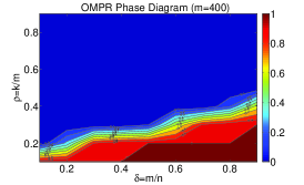
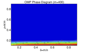
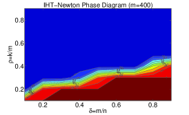
(a) OMPR	(b) OMP	(c) IHT-Newton

Figure 1: Phase Transition Diagrams for different methods. Red represents high probability of success while blue represents low probability of success. Clearly, OMPR recovers correct solution for a much larger region of the plot than OMP and is comparable to IHT-Newton. (Best viewed in color)

6.1 Phase Transition Diagrams

We first compare different methods using phase transition diagrams which are commonly used in compressed sensing literature to compare different methods (MalekiD10, ). We first fix the number of measurements to be $m=400$ and generate different problem sizes by varying $\rho=k/m$ and $\delta=m/n$. For each problem size $(m,n,k)$, we generate random $m\times n$ Gaussian measurement matrices and $k$-sparse random vectors. We then estimate the probability of success of each of the method by applying the method to 100 randomly generated instances. A method is considered successful for a particular instance if it recovers the underlying $k$-sparse vector with at most $1\%$ relative error.

In Figure 1, we show the phase transition diagram of our OMPR method as well as that of OMP and IHT-Newton (with step size 1). The plots shows probability of successful recovery as a function of $\rho=m/n$ and $\delta=k/m$. Figure 1 (a) shows color coding of different success probabilities; red represents high probability of success while blue represents low probability of success. Note that for Gaussian measurement matrices, the RIP constant $\delta_{2k}$ is less than a fixed constant if and only if $m=Ck\log(n/k)$, where $C$ is a universal constant. This implies that $\frac{1}{\delta}=C\log\rho$ and hence a method that recovers for high $\delta_{2k}$ will have a large fraction in the phase transition diagram where successful recovery probability is high. We observe this phenomenon for both OMPR and IHT-Newton method which is consistent with their respective theoretical guarantees (see Theorem 4). On the other hand, as expected, the phase transition diagram of OMP has a negligible fraction of the plot that shows high recovery probability.

6.2 Performance for Noisy or Under-sampled Observations

Next, we empirically compare performance of OMPR to various existing compressed sensing methods. As shown in the phase transition diagrams in Figure 1, OMPR provides comparable recovery to the IHT-Newton method for noiseless cases. Here, we show that OMPR is fairly robust under the noisy setting as well as in the case of under-sampled observations, where the number of observations is much smaller than what is required for exact recovery.

For this experiment, we generate random Gaussian measurement matrix of size $m=200,n=3000$. We then generate random binary vector $x$ of sparsity $k$ and add Gaussian noise to it. Figure 2 (a) shows recovery error ($\|Ax-b\|$) incurred by various methods for increasing $k$ and noise level of $10\%$. Clearly, our method outperforms the existing methods, perhaps a consequence of guaranteed convergence to a local minima for fixed step size $\eta=1$. Similarly, Figure 2 (b) shows recovery error incurred by various methods for fixed $k=50$ and varying noise level. Here again, our method outperforms existing methods and is more robust to noise. Finally, in Figure 2 (c) we show difference in error incurred along with confidence interval (at $95\%$ signficance level) by IHT-Newton and OMPR for varying levels of noises and $k$. Our method is better than IHT-Newton (at $95\%$ signficance level) in terms of recovery error in around 30 cells of the table, and is not worse in any of the cells but one.

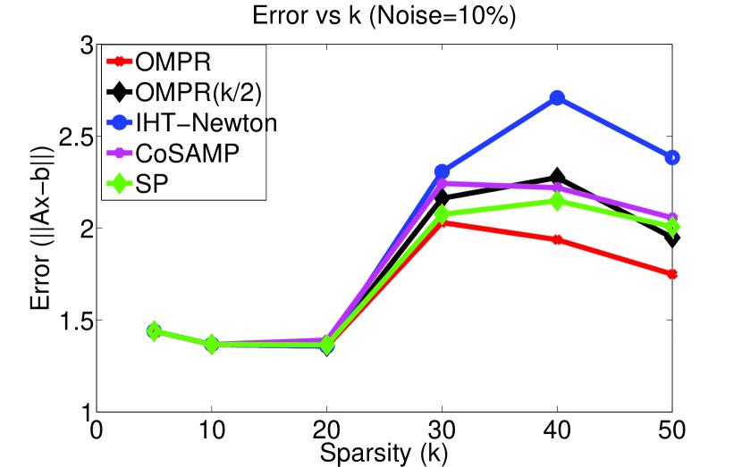
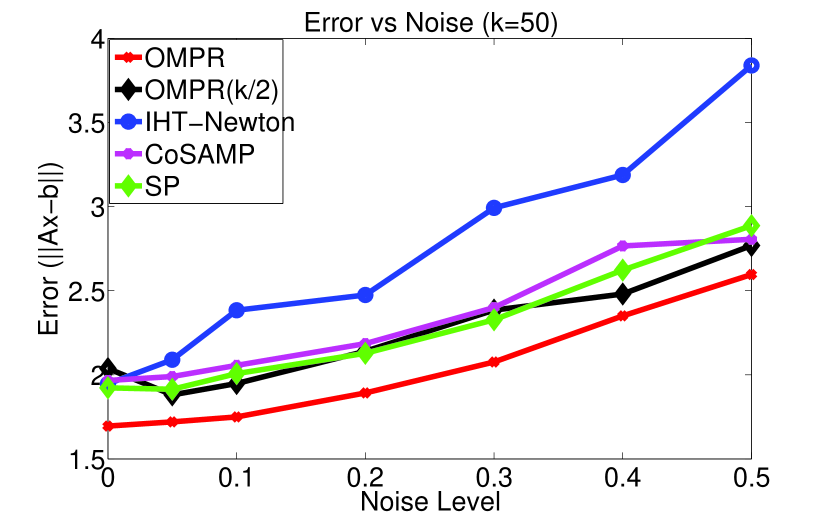
		Noise/ k 10 30 50 0.00 0.00(0.0) -0.21(0.6) 0.25(0.3) 0.05 0.00(0.0) 0.13(0.3) 0.37(0.3) 0.10 0.00(0.0) 0.28(0.3) 0.63(0.4) 0.20 0.03(0.0) 0.62(0.2) 0.58(0.5) 0.30 0.18(0.1) 0.92(0.3) 0.92(0.6) 0.40 0.31(0.1) 1.19(0.3) 0.84(0.5) 0.50 0.37(0.1) 1.48(0.3) 1.24(0.6)
(a)	(b)	(c)

Figure 2: Error in recovery ($\|Ax-b\|$) of $n=3000$ dimensional vectors from $m=200$ measurements. (a): Error incurred by various methods as the sparsity level $k$ increases. Note that OMPR  incurs the least error as it provably converges to at least a local minima for fixed step size $\eta=1$. (b): Error incurred by various methods as the noise level increases. Here again OMPR performs significantly better than the existing methods. (c): Difference in error incurred by IHT-Newton and OMPR , i.e., Error(IHT-Newton)-Error(OMPR ). Numbers in bracket denote confidence interval at 95% significance level.

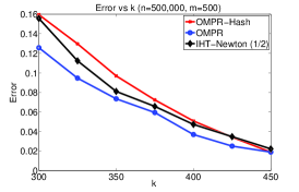
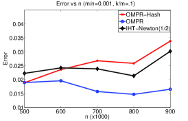
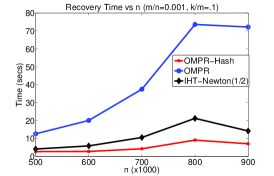
(a)	(b)	(c)

Figure 3: (a): Error ($\|Ax-b\|$) incurred by various methods as $k$ increases. The measurements $b=Ax$ are computing by generating $x$ with support size $m/10$. (b),(c): Error incurred and time required by various methods to recover vectors of support size $0.1m$ as $n$ increases. IHT-Newton(1/2) refers to the IHT-Newton method with step size $\eta=1/2$.

6.3 Performance of LSH based implementation

Next, we empirically study recovery properties of our LSH based implementation of OMPR ( OMPR-Hash ) in the following real-time setup: Generate a random measurement matrix from the Gaussian ensemble and construct hash tables offline using hash functions specified in Section 5. Next, during the reconstruction stage, measurements arrive one at a time and the goal is to recover the underlying signal accurately in real-time.For our experiments, we generate measurements using random sparse vectors and then report recovery error $\|Ax-b\|$ and computational time required by each of the method averaged over $20$ runs.

In our first set of experiments, we empirically study the performance of different methods as $k$ increases. Here, we fix $m=500$, $n=500,000$ and generate measurements using $n$-dimensional random vectors of support set size $m/10$. We then run different methods to estimate vectors $x$ of support size $k$ that minimize $\|Ax-b\|$. For our OMPR-Hash method, we use $s=20$ bits hash-keys and generate $q=\sqrt{n}$ hash-tables. Figure 3 (a) shows the error incurred by OMPR , OMPR-Hash , and IHT-Newton for different $k$ (recall that $k$ is an input to both OMPR and IHT-Newton). Note that although OMPR-Hash performs an approximation at each step, it is still able to achieve error similar to OMPR and IHT-Newton. Also, note that since the number of measurements are not enough for exact recovery by the IHT-Newton method, it typically diverges after a few steps. As a result, we use IHT-Newton with step size $\eta=1/2$ which is always guaranteed to monotonically converge to at least a local minima (see Theorem 4). In contrast, in OMPR and OMPR-Hash can always set step size $\eta$ aggressively to be $1$.

Next, we evaluate OMPR-Hash as dimensionality of the data $n$ increases. For OMPR-Hash , we use $s=\log_{2}(n)$ hash-keys and $q=\sqrt{n}$ hash-tables. Figures 3(b) and (c) compare error incurred and time required by OMPR-Hash with OMPR and IHT-Newton. Here again we use step size $\eta=1/2$ for IHT-Newton as it does not converge for $\eta=1$. Note that OMPR-Hash is an order of magnitude faster than OMPR while incurring slightly higher error. OMPR-Hash is also nearly $2$ times faster than IHT-Newton.

Appendix A Proofs related to OMPR: Exact Recovery Case

Let us denote the objective function by $f(x)=\frac{1}{2}\|Ax-b\|^{2}$. Let $I_{t}$ denote the support set of $x^{t}$ and $I^{\star}$ be the support set of $x^{\star}$. Define the sets

$$FA_{t} =I_{t}\backslash I^{\star}$$ (false alarms)

$$MD_{t} =I^{\star}\backslash I_{t}$$ (missed detections)

$$CO_{t} =I_{t}\cap I^{\star} \text{(correct detections)}\ .$$

As the algorithms proceed, elements get in and move in and out of the current set $I_{t}$. Let us give names to the set of found and lost elements as we move from $I_{t}$ to ${I_{t+1}}$:

$$F_{t} ={I_{t+1}}\backslash I_{t}$$ (found)

$$L_{t} =I_{t}\backslash{I_{t+1}} \text{(lost)}\ .$$

We first state two technical lemmas that we will need. These can be found in [19].

Lemma 13.

For any $S\subset[n]$, we have,

$$\|I-A_{S}^{T}A_{S}\|\leq\delta_{|S|}.$$

Lemma 14.

For any $S,T\subset[n]$ such that $S\cap T=\emptyset$, we have,

$$\|A_{S}^{T}A_{T}\|_{2}\leq\delta_{|S\cap T|}.$$

Proof of Theorem 3

Lemma 15.

Let $\delta_{2k}<1-\frac{1}{2\eta}$. Then, in OMPR ($l$),

$$0<2(2\eta-\frac{1}{1-\delta_{2k}})f(x^{t})\leq\|z_{MD_{t}}^{t+1}\|^{2}-\|x_{FA_{t}}^{t}\|^{2}.$$

Proof.

Since $x_{I_{t}}^{t}$ is the solution to the least squares problem $\min_{x}\|A_{I_{t}}x-b\|^{2}$,

$$A_{I_{t}}^{T}(A_{I_{t}}x_{I_{t}}^{t}-b)=\mathbf{0}.$$ (6)

Now, note that

$$f(x^{t}) =\frac{1}{2}\|A_{I_{t}}x_{I_{t}}^{t}-A_{I^{\star}}x_{I^{\star}}^{\star}\|^{2},$$

$$=\frac{1}{2}((x_{I_{t}}^{t})^{T}A_{I_{t}}^{T}(A_{I_{t}}x^{t}-A_{I^{\star}}x^{*})-(x_{I^{\star}}^{\star})^{T}A_{I^{\star}}^{T}(A_{I_{t}}x^{t}-A_{I^{\star}}x^{*})),$$

$$=-\frac{1}{2}(x_{MD_{t}}^{\star})^{T}A_{MD_{t}}^{T}(A_{I_{t}}x_{I_{t}}^{t}-A_{I^{\star}}x_{I^{\star}}^{\star}),\qquad\text{by \eqref{eq:ls}}$$

$$=\frac{1}{2\eta}(x_{MD_{t}}^{\star})^{T}z_{MD_{t}}^{t+1}.\qquad\text{by \eqref{eq:zt}}$$ (7)

Hence,

$$\|x_{MD_{t}}^{\star}-z_{MD_{t}}^{t+1}\|^{2} =\|x_{MD_{t}}^{\star}\|^{2}+\|z_{MD_{t}}^{t+1}\|^{2}-2(x_{MD_{t}}^{\star})^{T}z_{MD_{t}}^{t+1}$$

$$=\|x_{MD_{t}}^{\star}\|^{2}+\|z_{MD_{t}}^{t+1}\|^{2}-4\eta f(x^{t}).$$ (8)

That is,

$$4\eta f(x^{t}) \leq\|x_{MD_{t}}^{\star}\|^{2}+\|z_{MD_{t}}^{t+1}\|^{2},$$

$$\leq\|x_{MD_{t}}^{\star}\|^{2}+\|x_{FA_{t}}^{t}\|^{2}+\|x_{CO_{t}}^{t}-x_{CO_{t}}^{\star}\|^{2}-\|x_{FA_{t}}^{t}\|^{2}+\|z_{MD_{t}}^{t+1}\|^{2},$$

$$=\|x^{t}-x^{\star}\|^{2}+\|z_{MD_{t}}^{t+1}\|^{2}-\|x_{FA_{t}}^{t}\|^{2},$$

$$\leq\frac{1}{1-\delta_{2k}}\|A(x^{t}-x^{\star})\|^{2}+\|z_{MD_{t}}^{t+1}\|^{2}-\|x_{FA_{t}}^{t}\|^{2},\qquad\text{by RIP}$$

$$=\frac{2}{1-\delta_{2k}}f(x^{t})+\|z_{MD_{t}}^{t+1}\|^{2}-\|x_{FA_{t}}^{t}\|^{2},$$

where the third line follows from the fact that $MD_{t}$, $FA_{t}$, and $CO_{t}$ are disjoint sets.

As $f(x^{t})>0$ and $\delta_{2k}<1-\frac{1}{2\eta}$, the above inequality implies

$$0<2(2\eta-\frac{1}{1-\delta_{2k}})f(x^{t})\leq\|z_{MD_{t}}^{t+1}\|^{2}-\|x_{FA_{t}}^{t}\|^{2}.$$

∎

Next, we provide a lemma that bounds the function value $f(x^{t})$ in terms of missed detections $MD_{t}$ and also $z_{MD_{t}}^{t+1}$.

Lemma 16.

Let $f(x^{t})=\frac{1}{2}\|Ax^{t}-b\|^{2}$, $b=Ax^{*}$, $\delta_{2k}<1-\frac{1}{2\eta}$ and $\eta<1$. Then, at each step,

$$\frac{(1-\eta)^{2}}{\eta}\|x_{MD_{t}}^{\star}\|^{2}\ \leq\ f(x^{t})\ \leq\ \frac{1}{4\eta(1-\eta)^{2}}\|z_{MD_{t}}^{t+1}\|^{2}$$ (9)

Proof.

Now, using Lemma 2 of [4] with $I=MD_{t}$, $J=I_{t}$, $y=A_{MD_{t}}x^{\star}_{MD_{t}}$ we get

$$f(x^{t}) =\tfrac{1}{2}\|Ax^{t}-b\|^{2}$$

$$=\tfrac{1}{2}\|A_{I_{t}}(x^{t}-x^{\star})_{I_{t}}-A_{MD_{t}}x^{\star}_{MD_{t}}\|^{2}$$ (10)

$$\geq\tfrac{1}{2}\left(1-\frac{\delta_{2k}}{1-\delta_{k}}\right)^{2}\|A_{MD_{t}}x^{\star}_{MD_{t}}\|^{2}$$

$$\geq\tfrac{1}{2}\left(1-\frac{\delta_{2k}}{1-\delta_{k}}\right)^{2}(1-\delta_{k})\|x_{MD_{t}}^{\star}\|^{2}\qquad\text{by RIP}$$

$$\geq\tfrac{1}{2}\left(1-\frac{\delta_{2k}}{1-\delta_{2k}}\right)^{2}(1-\delta_{2k})\|x_{MD_{t}}^{\star}\|^{2}$$

$$\geq\frac{(1-2\delta_{2k})^{2}}{2(1-\delta_{2k})}\|x_{MD_{t}}^{\star}\|^{2}$$ (11)

The assumption that $\delta_{2k}<1-\tfrac{1}{2\eta}$ and $\eta<1$ implies that $\delta_{2k}<1-\tfrac{1}{2\eta}<1/2$. The function $\alpha\mapsto(1-2\alpha)^{2}/(2(1-\alpha))$ is decreasing on $[0,1/2]$ and hence (11) implies

$$f(x^{t})\geq\frac{\left(1-2(1-\frac{1}{2\eta})\right)^{2}}{2(1-1+\frac{1}{2\eta})}\|x_{MD_{t}}^{\star}\|^{2}=\frac{(1-\eta)^{2}}{\eta}\|x_{MD_{t}}^{\star}\|^{2}.$$ (12)

Next, using (7) and Cauchy-Schwarz inequality:

$$\|z_{MD_{t}}^{t+1}\|^{2}\geq 4\eta^{2}\frac{f(x^{t})^{2}}{\|x_{MD_{t}}^{\star}\|^{2}}.$$ (13)

The result now follows using the above equation with (12). ∎

Lemma 17.

Let $\delta_{2k}<1-\frac{1}{2\eta}$ and $1/2<\eta<1$. Then assuming $f(x^{t})>0$, at least one new element is found i.e. $F_{t}\neq\emptyset$. Furthermore, $\|y_{F_{t}}^{t+1}\|^{2}>\frac{l}{k}cf(x^{t})$, where $c=\min(4\eta(1-\eta)^{2},2(2\eta-\frac{1}{1-\delta_{2k}}))>0$ is a constant.

Proof.

We consider the following three exhaustive cases:

1. $|F_{t}|<l$ and $|F_{t}|<|MD_{t}|$: Let $S\subseteq|MD_{t}\backslash F_{t}|$, s.t., $|S|=|F_{t}|-|MD_{t}\cap F_{t}|$. Now,

   $$|S\cup(MD_{t}\cap F_{t})|=|F_{t}|,\ \ \ |(MD_{t}\backslash F_{t})\backslash S|=|MD_{t}|-|F_{t}|.$$

   Now, as $y_{F_{t}}$ consists of top $F_{t}$ elements of $z_{MD_{t}}^{t+1}$:

   $$\|z^{t+1}_{S\cup(MD_{t}\cap F_{t})}\|^{2}\leq\|y_{F_{t}}\|^{2}.$$ (14)

   Furthermore, since $|F_{t}|<l$, hence every element of $z^{t+1}_{MD_{t}\backslash F_{t}}$ is smaller in magnitude than every element of $x^{t}_{FA_{t}\backslash L_{t}}$, otherwise that element should have been included in $F_{t}$. Furthermore, $|MD_{t}|-|F_{t}|=|FA_{t}|-|L_{t}|\leq|FA_{t}\backslash L_{t}|$. Hence,

   $$\|z^{t+1}_{(MD_{t}\backslash F_{t})\backslash S}\|^{2}\leq\|x^{t}_{FA_{t}\backslash L_{t}}\|^{2}\leq\|x^{t}_{FA_{t}}\|^{2},$$ (15)

   Adding (14) and (15), we get:

   $$\|z^{t+1}_{MD_{t}}\|^{2}\leq\|y_{F_{t}}^{t+1}\|^{2}+\|x^{t}_{FA_{t}}\|^{2}.$$ (16)

   Using above equation along with Lemma 15, we get:

   $$\|y_{F_{t}}^{t+1}\|^{2}\geq 2\left(2\eta-\frac{1}{1-\delta_{2k}}\right)f(x^{t}).$$ (17)

   Now, note that if $|F_{t}|=0$, then $y_{F_{t}}^{t+1}=0$ implying that $f(x^{t})=0$. Hence, at least one new element is added, i.e., $y_{F_{t}}^{t+1}\neq\emptyset$.

2. $|F_{t}|=l<|MD_{t}|$: By definition of $y_{F_{t}}^{t+1}$:

   $$\frac{\|y_{F_{t}}^{t+1}\|^{2}}{|F_{t}|}\geq\frac{\|z_{MD_{t}}^{t+1}\|^{2}}{|MD_{t}|}.$$

   Hence, using Lemma 16 and the fact that $|F_{t}|=l$:

   $$\|y_{F_{t}}^{t+1}\|^{2}\geq\frac{l}{|MD_{t}|}4\eta(1-\eta)^{2}f(x^{t})\geq\frac{l}{k}4\eta(1-\eta)^{2}f(x^{t}),$$ (18)

   as $|MD_{t}|\leq k$.

3. $|F_{t}|\geq|MD_{t}|$: Since, $y_{F_{t}}^{t+1}$ is the top most elements of $z^{t+1}$. Hence, assuming $|F_{t}|\geq|MD_{t}|$,

   $$\|y_{F_{t}}^{t+1}\|^{2}\geq\|z_{MD_{t}}^{t+1}\|^{2}.$$

   Now, using Lemma 16:

   $$\|y_{F_{t}}^{t+1}\|^{2}\geq 4\eta(1-\eta)^{2}f(x^{t}).$$ (19)

We get the lemma by combining bounds for all the three cases, i.e., (17), (18), (19). ∎

Now we give a complete proof of Theorem 4.

Proof.

We have,

$$f(y^{t+1})-f(x^{t}) =(y^{t+1}-x^{t})^{T}A^{T}A(x^{t}-x^{\star})+1/2\|A(y^{t+1}-x^{t})\|^{2},$$

$$\leq(y^{t+1}-x^{t})^{T}A^{T}A(x^{t}-x^{\star})+\frac{(1+\delta_{2l})}{2}(\|y_{F_{t}}^{t+1}\|^{2}+\|x_{L_{t}}^{t}\|^{2}).$$ (20)

where the second inequality follows by using the fact that $y^{t+1}_{{I_{t+1}}\cap I_{t}}=x^{t}_{{I_{t+1}}\cap I_{t}}$ and using RIP of order $2l$ (since $|\operatorname{supp}(y^{t+1}-x^{t})|=|F_{t}\cup L_{t}|\leq 2l$).

Since $x^{t}_{I_{t}}$ is obtained using least squares,

$$A^{T}_{I_{t}}A(x^{t}-x^{\star})=\mathbf{0}.$$

Thus, $A^{T}_{L_{t}}A(x^{t}-x^{\star})=\mathbf{0}$, because $L_{t}\subseteq I_{t}$. Next, note that

$$y_{F_{t}}^{t+1}=-\eta A_{F_{t}}^{T}A(x^{t}-x^{\star}).$$

Hence,

$$f(y^{t+1})-f(x^{t}) \leq\left(\frac{1+\delta_{2l}}{2}-\frac{1}{\eta}\right)\|y_{F_{t}}^{t+1}\|^{2}+\frac{1+\delta_{2l}}{2}\|x_{L_{t}}^{t}\|^{2}.$$ (21)

Furthermore, since $y^{t+1}$ is chosen based on the $k$ largest entries in $z^{t+1}_{J_{t+1}}$, we have,

$$\|y_{F_{t}}^{t+1}\|^{2}=\|z^{t+1}_{F_{t}}\|^{2}\geq\|z^{t+1}_{L_{t}}\|^{2}=\|x_{L_{t}}^{t}\|^{2}\ .$$

Plugging this into (21), we get:

$$f(y^{t+1})-f(x^{t})\leq\left(1+\delta_{2l}-\frac{1}{\eta}\right)\|y_{F_{t}}^{t+1}\|^{2}\ .$$

Now, using Lemma 17, $\|y_{F_{t}}^{t+1}\|^{2}\geq\frac{l}{k}cf(x^{t})$ and therefore,

$$f(x^{t+1})-f(x^{t})\leq f(y^{t+1})-f(x^{t})\leq-\alpha\frac{l}{k}f(x^{t})$$

where $\alpha=c\left(1+\delta_{2l}-\frac{1}{\eta}\right)>0$ since $\eta(1+\delta_{2l})<1$. Hence,

$$f(x^{t+1})\leq(1-\alpha\frac{l}{k})f(x^{t})\leq e^{-\alpha\frac{l}{k}}f(x^{t}).$$

The above inequality shows that at each iteration OMPR ($l$) reduces the objective function value by a fixed multiplicative factor. Furthermore, if $x^{0}$ is chosen to have entries bounded by $1$, then $f(x^{0})\leq(1+\delta_{2k})k$. Hence, after $O(\frac{k}{l}\log((1+\delta_{2k})k/\epsilon))$ iterations, the function value reduces to $\epsilon$, i.e., $f(x^{t})\leq\epsilon$. ∎

Appendix B Proofs related to the LSH Section

Lemma 18.

Let $\|x\|=1$ for all points $x$ in our database. Let $x^{*}$ be the nearest neighbor to $\bm{r}$ in $L_{2}$ distance metric, and let $\bm{r}^{T}x^{*}\geq c>0$. Then, a $(1+\alpha\epsilon)$-nearest neighbor to $\bm{r}$ is also a $(1-\epsilon)$-similar neighbor to $\bm{r}$, where $\alpha\leq\frac{2c}{1+\bm{r}^{T}\bm{r}-2c}$.

Proof.

Let $x^{\prime}$ be a $(1+\alpha\epsilon)$-nearest neighbor to $\bm{r}$, then:

$$\|x^{\prime}-\bm{r}\|^{2}\leq(1+\alpha\epsilon)\|x^{*}-\bm{r}\|^{2}.$$

Using $\|x^{\prime}\|=\|x^{*}\|=1$ and simplifying, we get:

$$\bm{r}^{T}x^{\prime} \geq(1-\epsilon)\bm{r}^{T}x^{*}+(\alpha+1)\epsilon\bm{r}^{T}x^{*}-\frac{\alpha\epsilon}{2}(1+\bm{r}^{T}\bm{r}),$$

$$\geq(1-\epsilon)\bm{r}^{T}x^{*}+((\alpha+1)c-\frac{\alpha}{2}(1+\bm{r}^{T}\bm{r}))\epsilon.$$

Hence, $x^{\prime}$ is a $(1-\epsilon)$-approximate similar neighbor to $\bm{r}$ if:

$$(\alpha+1)c\geq\frac{\alpha}{2}(1+\bm{r}^{T}\bm{r}).$$

The result follows after simplification. ∎

We now provide a proof of Theorem 7.

Proof.

Let us first consider a single step of OMPR . Now, similar to Lemma 15, we can show that if $\delta_{2k}<1/4-\gamma$ and $\eta=1-\gamma$, $\gamma>0$, then $\|z_{MD_{t}}^{t+1}\|^{2}>\frac{3}{2}\|x_{FA_{t}}^{t}\|^{2}$. Setting $\epsilon=1-\sqrt{\frac{2}{3}}$, implies that $(1-\epsilon)\max|z_{MD_{t}}^{t+1}|\geq\min|x_{FA_{t}}^{t}|$, i.e., a $(1-\epsilon)$-similar neighbor to $\max|z_{MD_{t}}^{t+1}|$ will still lead to a constant decrease in the objective function.

So, the goal is to ensure that with probability $1-\delta$, $\delta>0$, for all the $O(k)$ iterations, our LSH method returns at least a $(1-\epsilon)$-similar neighbor to $\max|z_{MD_{t}}^{t+1}|$ where $\epsilon=1-\sqrt{\frac{2}{3}}$. To this end, we need to ensure that at each step $t$, LSH finds at least a $(1-\epsilon)$-similar neighbor to $\max|z_{MD_{t}}^{t+1}|$ with probability at least $1-\delta/k$. Using Lemma 18, we need to find a $(1+\alpha\epsilon)$-nearest neighbor to $\max|z_{MD_{t}}^{t+1}|$, where

$$\alpha\leq\frac{2c}{1+\bm{r}^{T}\bm{r}-2c},$$

and $\bm{r}^{T}x^{*}\geq c$. Using Lemma 17, $\alpha=O(1/k)$. Hence the result now follows using Theorem 6 (main text). ∎

Appendix C Extension to Noisy Case

In this section, we consider the noisy case in which our objective function is $f(x)=\tfrac{1}{2}\|Ax-b\|^{2}$, where $b=Ax^{*}+e$ and $e\in\mathbb{R}^{m}$ is the “noise” vector.

Let $I_{t}$ denote the support set of $x^{t}$ and $I^{\star}$ be the support set of $x^{\star}$. Define the sets

$$FA_{t} =I_{t}\backslash I^{\star}$$ (false alarms)

$$MD_{t} =I^{\star}\backslash I_{t}$$ (missed detections)

$$CO_{t} =I_{t}\cap I^{\star} \text{(correct detections)}\ .$$

Lemma 19.

Let $f(x^{t})\geq\frac{C}{2}\|e\|^{2}$ and $\delta_{2k}<1-\frac{1}{2D\eta}$, where $D=\frac{C-\sqrt{C}}{(\sqrt{C}+1)^{2}}$. Then,

$$\|z_{MD_{t}}^{t+1}\|^{2}-\|x_{FA_{t}}^{t}\|^{2}\geq cf(x^{t}),$$

where $c=2\frac{(\sqrt{C}+1)^{2}}{C}(2\eta D-\frac{1}{1-\delta_{2k}})>0$.

Proof.

Since $x_{I_{t}}^{t}$ is the solution to the least squares problem $\min_{x}\|A_{I_{t}}x-b\|^{2}$,

$$A_{I_{t}}^{T}(A_{I_{t}}x_{I_{t}}^{t}-b)=0.$$ (22)

Now, note that

$$f(x^{t}) =\frac{1}{2}\|A_{I_{t}}x_{I_{t}}^{t}-b\|^{2},$$

$$=\frac{1}{2}((x_{I_{t}}^{t})^{T}A_{I_{t}}^{T}(A_{I_{t}}x^{t}-b)-b^{T}(A_{I_{t}}x^{t}-b)),$$

$$=-\frac{1}{2}b^{T}(A_{I_{t}}x_{I_{t}}^{t}-b),$$

$$=-\frac{1}{2}(x^{*}_{MD_{t}})^{T}A_{MD_{t}}^{T}(A_{I_{t}}x_{I_{t}}^{t}-b)-\frac{1}{2}e^{T}(A_{I_{t}}x_{I_{t}}^{t}-b),$$

$$=\frac{1}{2\eta}(x_{MD_{t}}^{\star})^{T}z_{MD_{t}}^{t+1}-\frac{1}{2}e^{T}(A_{I_{t}}x_{I_{t}}^{t}-b),$$ (23)

where the third equality follows from (22).

Now,

$$\|x_{MD_{t}}^{\star}-z_{MD_{t}}^{t+1}\|^{2} =\|x_{MD_{t}}^{\star}\|^{2}+\|z_{MD_{t}}^{t+1}\|^{2}-2(x_{MD_{t}}^{\star})^{T}z_{MD_{t}}^{t+1}$$

$$=\|x_{MD_{t}}^{\star}\|^{2}+\|z_{MD_{t}}^{t+1}\|^{2}-4\eta(f(x^{t})+\frac{1}{2}e^{T}(A_{I_{t}}x_{I_{t}}^{t}-b))$$ (24)

So,

$$0 \leq\|x_{MD_{t}}^{\star}\|^{2}+\|x_{FA_{t}}^{t}\|^{2}-\|x_{FA_{t}}^{t}\|^{2}+\|z_{MD_{t}}^{t+1}\|^{2}-4\eta(f(x^{t})+\frac{1}{2}e^{T}(A_{I_{t}}x_{I_{t}}^{t}-b)),$$

$$\leq\|x_{MD_{t}}^{\star}\|^{2}+\|x_{FA_{t}}^{t}\|^{2}+\|x_{CO_{t}}^{t}-x_{CO_{t}}^{\star}\|^{2}-\|x_{FA_{t}}^{t}\|^{2}+\|z_{MD_{t}}^{t+1}\|^{2}-4\eta(f(x^{t})+\frac{1}{2}e^{T}(A_{I_{t}}x_{I_{t}}^{t}-b)),$$

$$\leq\|x^{t}-x^{*}\|^{2}-\|x_{FA_{t}}^{t}\|^{2}+\|z_{MD_{t}}^{t+1}\|^{2}-4\eta(f(x^{t})+\frac{1}{2}e^{T}(A_{I_{t}}x_{I_{t}}^{t}-b)),$$

$$\leq\frac{1}{1-\delta_{2k}}\|A(x^{t}-x^{*})\|^{2}-\|x_{FA_{t}}^{t}\|^{2}+\|z_{MD_{t}}^{t+1}\|^{2}-4\eta(f(x^{t})+\frac{1}{2}e^{T}(A_{I_{t}}x_{I_{t}}^{t}-b)),$$

$$=\frac{1}{1-\delta_{2k}}\|A(x^{t}-x^{*})\|^{2}-\|x_{FA_{t}}^{t}\|^{2}+\|z_{MD_{t}}^{t+1}\|^{2}-4\eta(1-\frac{1}{\sqrt{C}})f(x^{t}).$$

Now, by assumption: $f(x^{t})\geq\frac{C}{2}\|e\|^{2}$. Hence,

$$\|A(x^{t}-x^{*})\| \leq\|A(x^{t}-x^{*})-e\|+\|e\|,$$

$$\|A(x^{t}-x^{*})\|^{2} \leq 2(1+\frac{1}{\sqrt{C}})^{2}f(x^{t}).$$

Hence,

$$2\left(2\eta(1-\frac{1}{\sqrt{C}})-\frac{1}{1-\delta_{2k}}(1+\frac{1}{\sqrt{C}})^{2}\right)f(x^{t})\leq\|z_{MD_{t}}^{t+1}\|^{2}-\|x_{FA_{t}}^{t}\|^{2}$$

Now, by assumption $\delta_{2k}<1-\frac{1}{2D\eta}$, where $D=\frac{(\sqrt{C}+1)^{2}}{C-\sqrt{C}}$. Hence, $c=2\frac{(\sqrt{C}+1)^{2}}{C}(2\eta D-\frac{1}{1-\delta_{2k}})>0$. ∎

Next, we provide a lemma that bounds the function value $f(x^{t})$ in terms of missed detection $MD_{t}$ and also $z_{MD_{t}}^{t+1}$.

Lemma 20.

Let $f(x^{t})=\frac{1}{2}\|Ax^{t}-b\|^{2}\geq\frac{C}{2}\|e\|^{2}$, $b=Ax^{*}+e$, $\delta_{2k}<1-\frac{1}{2D\eta}$ and $D=\frac{C-\sqrt{C}}{(\sqrt{C}+1)^{2}}$. Then, at each step,

$$\frac{(1-\eta)^{2}C}{\eta(\sqrt{C}+1)^{2}}\|x_{MD_{t}}^{\star}\|^{2}\ \leq\ f(x^{t})\ \leq\ \frac{1}{4\eta(1-\eta)^{2}}\frac{(\sqrt{C}+1)^{2}}{(\sqrt{C}-1)^{2}}\|z_{MD_{t}}^{t+1}\|^{2}$$ (25)

Proof.

First we lower bound $f(x^{t})$:

$$\sqrt{f(x^{t})} =\frac{1}{\sqrt{2}}\|Ax^{t}-Ax^{*}-e\|,$$

$$\geq\frac{1}{\sqrt{2}}\left(\|Ax^{t}-Ax^{*}\|-\|e\|\right),$$

$$\geq\frac{1}{\sqrt{2}}\left(\min_{x\>:\>x_{\bar{I}_{t}}=0}\|Ax-Ax^{*}\|-\|e\|\right),$$

$$\geq\frac{1}{\sqrt{2}}\left(\frac{(1-2\delta_{2k})}{\sqrt{(1-\delta_{2k})}}\|x_{MD_{t}}^{\star}\|-\|e\|\right),$$

where last equality follows from Lemma 16. Using the above inequality with $f(x^{t})\geq\frac{C}{2}\|e\|^{2}$, we get:

$$f(x^{t})\geq\frac{(1-2\delta_{2k})^{2}C}{2(1-\delta_{2k})(\sqrt{C}+1)^{2}}\|x_{MD_{t}}^{\star}\|^{2}.$$ (26)

The assumption that $\delta_{2k}<1-\tfrac{1}{2D\eta}$ and $D\eta<1$ implies that $\delta_{2k}<1-\tfrac{1}{2D\eta}<1/2$. The function $\alpha\mapsto(1-2\alpha)^{2}/(2(1-\alpha))$ is decreasing on $[0,1/2]$ and hence the above equation implies

$$f(x^{t})\geq\frac{(1-D\eta)^{2}}{D\eta}\|x_{MD_{t}}^{\star}\|^{2}.$$ (27)

Now, we upper bound $f(x^{t})$. Using definition of $f(x^{t})$:

$$\frac{1}{2\eta}(x_{MD_{t}}^{\star})^{T}z_{MD_{t}}^{t+1}=f(x^{t})+\frac{1}{2}e^{T}(A_{I_{t}}x_{I_{t}}^{t}-b).$$

Now, using Cauchy-Schwarz and $f(x^{t})\geq\frac{C}{2}\|e\|^{2}$,

$$\left|e^{T}(A_{I_{t}}x_{I_{t}}^{t}-b)\right|\leq\|e\|\|A_{I_{t}}x_{I_{t}}^{t}-b\|\leq\frac{2}{\sqrt{C}}f(x^{t}).$$

Hence,

$$\frac{1}{2\eta}\|x_{MD_{t}}^{\star}\|\|z_{MD_{t}}^{t+1}\|\geq\frac{1}{2\eta}(x_{MD_{t}}^{\star})^{T}z_{MD_{t}}^{t+1}\geq(1-\frac{1}{\sqrt{C}})f(x^{t}).$$

That is,

$$\|z_{MD_{t}}^{t+1}\|^{2}\geq 4\eta^{2}\left(1-\frac{1}{\sqrt{C}}\right)^{2}\frac{f(x^{t})^{2}}{\|x_{MD_{t}}^{\star}\|^{2}}\geq 4\eta(1-D\eta)^{2}\frac{(\sqrt{C}-1)^{2}}{CD}f(x^{t}),$$ (28)

where the second inequality follows from (27). ∎

Next, we present the following lemma that shows “enough” progress at each step:

Lemma 21.

Let $f(x^{t})\geq\frac{C}{2}\|e\|^{2}$, $\eta<1$ and $\delta_{2k}<1-\frac{1}{2D\eta}$, where $D=1-\frac{1}{\sqrt{C}-1}$. Then at least one new element is found i.e. $F_{t}\neq\emptyset$. Furthermore, $\|y_{F_{t}}^{t+1}\|>\frac{l}{k}\alpha f(x^{t})$, where $\alpha=\min(4\eta(1-D\eta)^{2}\frac{(\sqrt{C}-1)^{2}}{CD},2\frac{(\sqrt{C}+1)^{2}}{C}(2\eta D-\frac{1}{1-\delta_{2k}}))>0$ is a constant.

Proof.

As for the exact case, we analyse the following three exhaustive cases:

1. $|F_{t}|<l$ and $|F_{t}|<|MD_{t}|$: Here we use the exactly similar argument as the exact case to obtain the following inequality (see (16)):

   $$\|z^{t+1}_{MD_{t}}\|^{2}\leq\|y_{F_{t}}^{t+1}\|^{2}+\|x^{t}_{FA_{t}}\|^{2}.$$ (29)

   Using Lemma 19, we get:

   $$\|y_{F_{t}}^{t+1}\|^{2}\geq cf(x^{t}),$$ (30)

   where $c$ is as defined in Lemma 19. Now, note that if $|F_{t}|=0$, then $y_{F_{t}}^{t+1}=0$ implying that $f(x^{t})=0$. Hence, at least one new element is added, i.e., $y_{F_{t}}^{t+1}\neq\emptyset$.

2. $|F_{t}|=l<|MD_{t}|$: By definition of $y_{F_{t}}^{t+1}$:

   $$\frac{\|y_{F_{t}}^{t+1}\|^{2}}{|F_{t}|}\geq\frac{\|z_{MD_{t}}^{t+1}\|^{2}}{|MD_{t}|}.$$

   Hence, using Lemma 20 and the fact that $|F_{t}|=l$:

   $$\|y_{F_{t}}^{t+1}\|^{2}\geq\frac{l}{|MD_{t}|}4\eta(1-D\eta)^{2}\frac{(\sqrt{C}-1)^{2}}{CD}f(x^{t})\geq\frac{l}{k}4\eta(1-D\eta)^{2}\frac{(\sqrt{C}-1)^{2}}{CD}f(x^{t}),$$ (31)

   as $|MD_{t}|\leq k$.

3. $|F_{t}|\geq|MD_{t}|$: Since, $y_{F_{t}}^{t+1}$ is the top most elements of $z^{t+1}$. Hence, assuming $|F_{t}|\geq|MD_{t}|$,

   $$\|y_{F_{t}}^{t+1}\|^{2}\geq\|z_{MD_{t}}^{t+1}\|^{2}.$$

   Now, using Lemma 20:

   $$\|y_{F_{t}}^{t+1}\|^{2}\geq 4\eta(1-D\eta)^{2}\frac{(\sqrt{C}-1)^{2}}{CD}f(x^{t}).$$ (32)

We get the lemma by combining bounds for all the three cases, i.e., (30), (31), (32). ∎

Now, we provide a proof of Theorem 2.

Proof.

We have,

$$f(y^{t+1})-f(x^{t}) =(y^{t+1}-x^{t})^{T}A^{T}(Ax^{t}-b)+1/2\|A(y^{t+1}-x^{t})\|^{2},$$

$$\leq(y^{t+1}-x^{t})^{T}A^{T}(Ax^{t}-b)+\frac{(1+\delta_{2l})}{2}(\|y_{F_{t}}^{t+1}\|^{2}+\|x_{L_{t}}^{t}\|^{2}).$$ (33)

where the second inequality follows by using the fact that $y^{t+1}_{{I_{t+1}}\cap I_{t}}=x^{t}_{{I_{t+1}}\cap I_{t}}$ and using RIP of order $2l$ (since $|\operatorname{supp}(y^{t+1}-x^{t})|=|F_{t}\cup L_{t}|\leq 2l$).

Since $x^{t}_{I_{t}}$ is obtained using least squares,

$$A^{T}_{I_{t}}(Ax^{t}-b)=\mathbf{0}.$$

That is, $A^{T}_{L_{t}}(Ax^{t}-b)=\mathbf{0}$, because $L_{t}\subseteq I_{t}$. Next, note that

$$y_{F_{t}}^{t+1}=-\eta A_{F_{t}}^{T}(Ax^{t}-b).$$

Hence,

$$f(y^{t+1})-f(x^{t}) \leq\left(\frac{1+\delta_{2l}}{2}-\frac{1}{\eta}\right)\|y_{F_{t}}^{t+1}\|^{2}+\frac{1+\delta_{2l}}{2}\|x_{L_{t}}^{t}\|^{2}.$$ (34)

Furthermore, since $y^{t+1}$ is chosen based on largest entries in $z^{t+1}_{J_{t+1}}$, we have,

$$\|y_{F_{t}}^{t+1}\|^{2}=\|z^{t+1}_{F_{t}}\|^{2}\geq\|z^{t+1}_{L_{t}}\|^{2}=\|x_{L_{t}}^{t}\|^{2}\ .$$

Plugging this into (34), we get:

$$f(y^{t+1})-f(x^{t})\leq\left(1+\delta_{2l}-\frac{1}{\eta}\right)\|y_{F_{t}}^{t+1}\|^{2}\ .$$

Now, using Lemma 21, $\|y_{F_{t}}^{t+1}\|^{2}\geq\alpha f(x^{t})>0$ and therefore,

$$f(x^{t+1})-f(x^{t}) \leq f(y^{t+1})-f(x^{t})$$

$$\leq-c^{\prime}\frac{l}{k}f(x^{t})\ ,$$

where $c^{\prime}=\frac{1-\eta(1+\delta_{2l})}{\eta(1+\delta_{2l})}\,\alpha>0$ since $\eta(1+\delta_{2l})<1$. The above inequality shows that at each iteration OMPR ($l$) reduces the objective function value by a fixed multiplicative factor. Furthermore, if $x^{0}$ is chosen to have entries bounded by $1$, then $f(x^{0})\leq O((1+\delta_{2k})k+\|e\|^{2})$. Hence, after $O(\frac{k}{l}\log((k+\|e\|^{2})/\epsilon))$ iterations, the function value reduces to $C\|e\|^{2}/2+\epsilon$. ∎

Appendix D Analysis of 2-stage Algorithms

In this section, we consider the family of two-stage hard thresholding algorithms (see Algorithm 3) introduced by [17].

Algorithm 3 Two-stage($l$)

1:  Input: matrix $A$, vector $b$, sparsity level $k$

2:  Initialize $x^{1}$

3:  for $t=1$ to $T$ do

4:     $\mathrm{top}_{t+1}\leftarrow$ indices of top $l$ elements of $|A^{T}(Ax^{t}-b)|$

5:     $J_{t+1}\leftarrow I_{t}\cup\mathrm{top}_{t+1}$

6:     $z^{t+1}_{J_{t+1}}\leftarrow A_{J_{t+1}}\backslash b,\ z^{t+1}_{\bar{J}_{t+1}}\leftarrow\mathbf{0}$

7:     $y^{t+1}\leftarrow H_{k}\left(z^{t+1}\right)$

8:     ${I_{t+1}}\leftarrow\operatorname{supp}(y^{t+1})$

9:     $x^{t+1}_{I_{t+1}}\leftarrow A_{{I_{t+1}}}\backslash b,\ x^{t+1}_{\bar{I}_{t+1}}\leftarrow\mathbf{0}$

10:  end for

We now provide a simple analysis for the general two-stage hard thresholding algorithms. We first present a few technical lemmas that we will need for our proof.

Lemma 22.

Let $b=Ax^{\star}$, where $I^{*}=\operatorname{supp}(x^{\star})$. Also, let $x=\operatorname*{argmin}_{\operatorname{supp}(x)=I}\|Ax-b\|^{2}$. Then,

$$\sqrt{\|(x-x^{\star})_{I\cap I^{*}}\|^{2}+\|x_{I\backslash I^{*}}\|^{2}}=\|(x-x^{\star})_{I}\|\leq\frac{\delta_{|I\cup I^{*}|}}{\sqrt{1-\delta_{|I\cup I^{*}|}^{2}}}\|x^{\star}_{I^{*}\backslash I}\|$$

Proof.

A similar inequality appears in [10] and we rewrite the proof here. Since $x_{I}$ is the solution to $\min_{u}\|A_{I}u-b\|^{2}$,

$$A_{I}^{T}(A_{I}x_{I}-b)=0.$$ (35)

In the exact case, $b=Ax^{*}$. Hence,

$$\|(x-x^{\star})_{I}\|^{2}=\left[(x-x^{\star})_{I}\ \ 0\right]^{T}\left[\begin{matrix}(x-x^{\star})_{I}\\ -x^{\star}_{I^{*}\backslash I}\end{matrix}\right]$$ (36)

Now, using (35):

$$0=\left[(x-x^{\star})_{I}\ \ 0\right]^{T}A_{G}^{T}A_{G}\left[\begin{matrix}(x-x^{\star})_{I}\\ -x^{\star}_{I^{*}\backslash I}\end{matrix}\right],$$ (37)

where $G=[I\ \ I^{*}\backslash I]$. Subtracting (37) from (36) we get,

$$\|(x-x^{\star})_{I}\|^{2} =\left[(x-x^{\star})_{I}\ \ 0\right]^{T}(I-A_{G}^{T}A_{G})\left[\begin{matrix}(x-x^{\star})_{I}\\ -x^{\star}_{I^{*}\backslash I}\end{matrix}\right],$$

$$\leq\delta_{2k}\|(x-x^{\star})_{I}\|\sqrt{\|(x-x^{\star})_{I}\|^{2}+\|x^{\star}_{I^{*}\backslash I}\|^{2}},$$ (38)

where the second inequality follows using Lemma 13. Lemma follows by just rearranging terms now. ∎

We now present our main theroem and its proof for two-stage thresholding algorithms.

Theorem 23.

Suppose the vector $x^{\star}\in\mathbb{R}^{n}$ is $k$-sparse and binary. Then Two-stage($l$) recovers $x^{\star}$ from measurements $b=Ax^{\star}$ in $O(k)$ iterations provided:

$$\delta_{2k+l}\leq.35$$

Proof.

As $z^{t+1}$ is the least squares solution over support set $J_{t+1}$, hence:

$$f(z^{t+1})-f(x^{t})\leq f(s^{t+1})-f(x^{t}),$$ (39)

where $s^{t+1}_{J_{t+1}}=(x^{t}-\eta A^{T}(Ax^{t}-b))_{J_{t+1}}$, $\eta=\frac{1}{1+\delta_{l}}$ and $s^{t+1}_{\bar{J}_{t+1}}=0$.

Now,

$$f(s^{t+1})-f(x^{t}) =(s^{t+1}-x^{t})^{T}A^{T}(Ax^{t}-b)+\frac{1}{2}\|As^{t+1}-Ax^{t}\|^{2}.$$ (40)

Now, as $x^{t}$ is the least squares solution over $I_{t}$. Hence, $A_{I_{t}}^{T}(Ax^{t}-b)=0$. Hence,

$$(s^{t+1}-x^{t})_{I_{t}}=0,\ \ \ (s^{t+1}-x^{t})_{\mathrm{top}_{t+1}}=-\eta A^{T}_{\mathrm{top}_{t+1}}(Ax^{t}-b),\ \ \ (s^{t+1}-x^{t})_{\bar{J}_{t+1}}=0.$$ (41)

Using (40) and (41):

$$f(s^{t+1})-f(x^{t}) =-\eta\|A^{T}_{\mathrm{top}_{t+1}}(Ax^{t}-b)\|^{2}+\frac{\eta^{2}}{2}\|A_{\mathrm{top}_{t+1}}A^{T}_{\mathrm{top}_{t+1}}(Ax^{t}-b)\|^{2},$$

$$\leq-\eta\|A^{T}_{\mathrm{top}_{t+1}}(Ax^{t}-b)\|^{2}+\frac{\eta^{2}(1+\delta_{l})}{2}\|A^{T}_{\mathrm{top}_{t+1}}(Ax^{t}-b)\|^{2},$$

$$=-\frac{\eta}{2}\|A^{T}_{\mathrm{top}_{t+1}}(Ax^{t}-b)\|^{2}.$$ (42)

Now, let $MD_{t}$ be the set of missed detections, i.e., $MD_{t}=I^{*}\backslash I^{t}$. Then, by definition of $\mathrm{top}_{t+1}$:

$$\|A^{T}_{\mathrm{top}_{t+1}}(Ax^{t}-b)\|^{2}\geq\min\left(1,\frac{l}{|MD_{t}|}\right)\|A^{T}_{MD_{t}}(Ax^{t}-b)\|^{2}.$$ (43)

Furthermore,

$$\|A^{T}_{MD_{t}}(Ax^{t}-b)\| =\|A^{T}_{MD_{t}}A_{MD_{t}}x^{*}_{MD_{t}}-A^{T}_{MD_{t}}A_{I_{t}}(x^{t}-x^{*})_{I_{t}}\|,$$

$$\geq\|A^{T}_{MD_{t}}A_{MD_{t}}x^{*}_{MD_{t}}\|-\|A^{T}_{MD_{t}}A_{I_{t}}(x^{t}-x^{*})_{I_{t}}\|,$$

$$\geq(1-\delta_{k})\|x^{*}_{MD_{t}}\|-\frac{\delta_{2k}^{2}}{\sqrt{1-\delta_{2k}^{2}}}\|x^{*}_{MD_{t}}\|,$$ (44)

where last inequality follows using Lemma 14 and Lemma 22.

Hence, using (42), (43), and (44):

$$f(z^{t+1})-f(x^{t})\leq f(s^{t+1})-f(x^{t})\leq-\frac{1}{2(1+\delta_{l})}\min\left(1,\frac{l}{|MD_{t}|}\right)\left(1-\delta_{k}-\frac{\delta_{2k}^{2}}{\sqrt{1-\delta_{2k}^{2}}}\right)^{2}\|x^{*}_{MD_{t}}\|^{2}.$$ (45)

Next, we upper bound increase in the objective function by removing $l$ elements from $z^{t+1}$.

$$f(y^{t+1})-f(z^{t+1}) =(y^{t+1}-z^{t+1})^{T}A^{T}(Az^{t+1}-b)+\frac{1}{2}\|Ay^{t+1}-Az^{t+1}\|^{2},$$

$$=\frac{1}{2}\|Ay^{t+1}-Az^{t+1}\|^{2},$$

$$\leq\frac{1+\delta_{l}}{2}\|z^{t+1}_{J_{t+1}\backslash I_{t+1}}\|^{2},$$ (46)

where the second equation follows as $z^{t+1}$ is a least squares solution, and both $y^{t+1},\ z^{t+1}$’s support is a subset of $J_{t+1}$. The third equation follows from RIP and the fact that $z^{t+1}_{I_{t+1}}=y^{t+1}_{I_{t+1}}$.

Now, using Lemma 22:

$$\|z^{t+1}_{J_{t+1}\backslash I^{*}}\|^{2}\leq\frac{\delta_{2k+l}^{2}}{1-\delta_{2k+l}^{2}}\|x^{*}_{I^{*}\backslash J_{t+1}}\|^{2}.$$ (47)

Furthermore, $|J_{t+1}\backslash I_{t+1}|=l\leq|J_{t+1}\backslash I^{*}|$. Hence, by definition of $I_{t+1}$,

$$\|z^{t+1}_{J_{t+1}\backslash I_{t+1}}\|^{2}\leq\frac{l}{|J_{t+1}\backslash I^{*}|}\|z^{t+1}_{J_{t+1}\backslash I^{*}}\|^{2}.$$

Using above equation and (47), we get:

$$\|z^{t+1}_{J_{t+1}\backslash I_{t+1}}\|^{2}\leq\frac{l}{|J_{t+1}\backslash I^{*}|}\frac{\delta_{2k+l}^{2}}{1-\delta_{2k+l}^{2}}\|x^{*}_{I^{*}\backslash J_{t+1}}\|^{2},$$ (48)

Also, $|J_{t+1}\backslash I^{*}|=l+|I^{*}\backslash J_{t+1}|\leq l+|MD_{t}|$. Using (46), (48), and the fact that $f(x^{t+1})\leq f(y^{t+1})$ and each $x^{*}_{I^{*}}=1$:

$$f(x^{t+1})-f(z^{t+1})\leq\frac{l}{l+|I^{*}\backslash J_{t+1}|}\frac{1+\delta_{l}}{2}\frac{\delta_{2k+l}^{2}}{1-\delta_{2k+l}^{2}}|I^{*}\backslash J_{t+1}|.$$ (49)

Adding (45) and (49), we get:

$$f(x^{t+1})-f(x^{t})\leq-\frac{1}{2(1+\delta_{l})}\left(\min\left(|MD_{t}|,l\right)\left(1-\delta_{k}-\frac{\delta_{2k}^{2}}{\sqrt{1-\delta_{2k}^{2}}}\right)^{2}-\frac{l\cdot|I^{*}\backslash J_{t+1}|}{l+|I^{*}\backslash J_{t+1}|}\frac{(1+\delta_{l})^{2}\delta_{2k+l}^{2}}{1-\delta_{2k+l}^{2}}\right).$$ (50)

Now, $\frac{l\cdot|I^{*}\backslash J_{t+1}|}{l+|I^{*}\backslash J_{t+1}|}\leq\min(l,|I^{*}\backslash J_{t+1}|)\leq\min(l,|MD_{t}|)$.

Hence,

$$f(x^{t+1})-f(x^{t})\leq-\frac{\min(l,|MD_{t}|)}{2(1+\delta_{l})}\left(\left(1-\delta_{k}-\frac{\delta_{2k}^{2}}{\sqrt{1-\delta_{2k}^{2}}}\right)^{2}-\frac{(1+\delta_{l})^{2}\delta_{2k+l}^{2}}{1-\delta_{2k+l}^{2}}\right).$$ (51)

Now consider:

$$\left(\left(1-\delta_{k}-\frac{\delta_{2k}^{2}}{\sqrt{1-\delta_{2k}^{2}}}\right)^{2}-\frac{(1+\delta_{l})^{2}\delta_{2k+l}^{2}}{1-\delta_{2k+l}^{2}}\right) \geq\frac{1}{1-\delta_{2k+l}^{2}}\left(((1-\delta_{2k+l})\sqrt{1-\delta_{2k+l}^{2}}-\delta_{2k+l}^{2})^{2}-(1+\delta_{2k+l})^{2}\delta_{2k+l}^{2}\right),$$

$$>0.01,$$ (52)

where the second inequality follows by substituting $\delta_{2k+1}\leq.35$.

Hence, using (51) and (52), we have:

$$f(x^{t+1})\leq f(x^{t})-\min(l,|MD_{t}|)\cdot 0.0001.$$ (53)

The above equation guarantees convergence to the optima in at least $O(k)$ steps although faster convergence can be shown for larger $k$. ∎

Corollary 24.

Cosamp converges to the optima provided

$$\delta_{4k}\leq 0.35.$$

Corollary 25.

Subspace-Pursuit converges to the optima provided

$$\delta_{3k}\leq 0.35.$$

Note that CoSamp’s analysis given by [19] requires $\delta_{4k}\leq 0.1$ while Subspace pursuit’s analysis given by [4] requires $\delta_{3k}\leq 0.205$. Note that our generic analysis provides significantly better guarantees for both the methods.

References

- [1] T. Blumensath and M. E. Davies. Iterative hard thresholding for compressed sensing. Applied and Computational Harmonic Analysis, 27(3):265–274, 2009.
- [2] E. J. Candes. The restricted isometry property and its implications for compressed sensing. Comptes Rendus Mathematique, 346(9-10):589–592, 2008.
- [3] E. J. Candes and T. Tao. Decoding by linear programming. IEEE Transactions on Information Theory, 51(12):4203–4215, 2005.
- [4] W. Dai and O. Milenkovic. Subspace pursuit for compressive sensing signal reconstruction. IEEE Transactions on Information Theory, 55(5):2230–2249, 2009.
- [5] M. A. Davenport and M. B. Wakin. Analysis of orthogonal matching pursuit using the restricted isometry property. IEEE Transactions on Information Theory, 56(9):4395–4401, 2010.
- [6] G. Davis, S. Mallat, and M. Avellaneda. Greedy adaptive approximation. Constr. Approx, 13:57–98, 1997.
- [7] D. Donoho. Compressed sensing. IEEE Trans. on Information Theory, 52(4):1289–1306, 2006.
- [8] D. Donoho, A. Maleki, and A. Montanari. Message passing algorithms for compressed sensing. Proceedings of the National Academy of Sciences USA, 106(45):18914–18919, 2009.
- [9] M. F. Duarte, M. A. Davenport, D. Takhar, J. N. Laska, T. Sun, K. F. Kelly, and R. G. Baranuik. Single-pixel imaging via compressive sampling. IEEE Signal Processing Magazine, 25(2):83–91, March 2008.
- [10] S. Foucart. Hard thresholding pursuit: an algorithm for compressive sensing, 2010. preprint.
- [11] S. Foucart. A note on guaranteed sparse recovery via -minimization. Applied and Computational Harmonic Analysis, 29(1):97–103, 2010.
- [12] A. Gionis, P. Indyk, and R. Motwani. Similarity search in high dimensions using hashing. In VLDB, 1999.
- [13] M. X. Goemans and D. P. Williamson. .879-approximation algorithms for MAX CUT and MAX 2SAT. In STOC, pages 422–431, 1994.
- [14] D. Hsu, S. M. Kakade, J. Langford, and T. Zhang. Multi-label prediction via compressed sensing. In NIPS, 2009.
- [15] P. Jain, R. Meka, and I. S. Dhillon. Guaranteed rank minimization via singular value projection. In NIPS, 2010.
- [16] A. Maleki. Convergence analysis of iterative thresholding algorithms. In Allerton Conference on Communication, Control and Computing, 2009.
- [17] A. Maleki and D. Donoho. Optimally tuned iterative reconstruction algorithms for compressed sensing. IEEE Journal of Selected Topics in Signal Processing, 4(2):330–341, 2010.
- [18] Q. Mo and Y. Shen. Remarks on the restricted isometry property in orthogonal matching pursuit algorithm, 2011. preprint arXiv:1101.4458.
- [19] D. Needell and J. A. Tropp. Cosamp: Iterative signal recovery from incomplete and inaccurate samples. Applied and Computational Harmonic Analysis, 26(3):301 – 321, 2009.
- [20] S. Negahban, P. Ravikumar, M. J. Wainwright, and B. Yu. A unified framework for high-dimensional analysis of -estimators with decomposable regularizers. In NIPS, 2009.
- [21] Y. C. Pati, R. Rezaiifar, and P. S. Krishnaprasad. Orthogonal matching pursuit: Recursive function approximation with applications to wavelet decomposition. In 27th Annu. Asilomar Conf. Signals, Systems, and Computers, volume 1, pages 40–44, 1993.
- [22] H. Rauhut. On the impossibility of uniform sparse reconstruction using greedy methods. Sampling Theory in Signal and Image Processing, 7(2):197–215, 2008.
- [23] S. Shalev-Shwartz, N. Srebro, and T. Zhang. Trading accuracy for sparsity in optimization problems with sparsity constraints. SIAM Journal on Optimization, 20:2807–2832, 2010.
- [24] J. Wright, Y. Ma, J. Mairal, G. Sapiro, T. S. Huang, and S. Yan. Sparse representation for computer vision and pattern recognition. Proceedings of the IEEE, 98(6):1031–1044, 2010.
- [25] T. Zhang. Adaptive forward-backward greedy algorithm for sparse learning with linear models. In NIPS, 2008.
- [26] T. Zhang. Sparse recovery with orthogonal matching pursuit under RIP, 2010. preprint arXiv:1005.2249.