Oil displacement through a porous medium with a temperature gradient

Abstract

We investigate the effect of a temperature gradient on oil recovery in a two-dimensional pore-network model. The oil viscosity depends on temperature as, $\mu_{o}=exp(B/T)$, where $B$ is a physico-chemical parameter depending on the type of oil, and $T$ is the temperature. A temperature gradient is applied across the medium in the flow direction. Initially, the porous medium is saturated with oil and, then, another fluid is injected. We have considered two cases representing different injection strategies. In the first case, the invading fluid viscosity is constant (finite viscosity ratio) while in the second one, the invading fluid is inviscid (infinite viscosity ratio). Our results show that, for the case of finite viscosity ratio, recovery increases with $\Delta T$ independently on strength or sign of the gradient. For an infinite viscosity ratio, a positive temperature gradient is necessary to enhance recovery. Moreover, we show that, for $\Delta T>0$, the percentage of oil recovery generally decreases (increases) with $B$ for a finite (infinite) viscosity ratio. Finally, we also extend our results for infinite viscosity ratio to a three-dimensional porous media geometry.

I Introduction

Thermal recovery processes have been used by petroleum companies as a strategic method to improve oil production from reservoirs. These processes consist, basically, in decreasing the oil viscosity (increasing the pressure) by increasing the temperature of the reservoir using a heat source Prats . In practice, this can be done by injecting a hot fluid (steam or water) into the reservoir. A method often called Steam or Hot-Water Injection has been mostly used by companies exploiting heavy oil reservoirs Craft ; Moore .

The temperature dependence of the oil viscosity is governed by physico-chemical parameters which can allow a reduction of oil viscosity by several orders of magnitude with only a modest increase of temperature Prats . In general, oil properties in the operational conditions of a reservoir field are very difficult to predict and can be very different for each type of oil or oil mixture. Therefore, their direct measurement is highly desirable for a better understanding of this phenomenon, and to improve the efficiency of the recovery.

Several approaches to model and simulate oil recovery have been utilized in the past. Some of them make use of the macroscopic description of conservation laws in a porous medium, simulating a whole reservoir, including injectors and producers wells Turta ; Kuhlman . Other authors use conservation laws under a more microscopic approach Andrade ; Ferer ; Ferer1 ; Andrade2 ; Andrade3 ; Auradou ; Andrade4 ; Andrade5 ; Sahimi ; Andrade6 ; Andrade7 ; Lenormand ; Andrade8 , where a portion of the porous medium can be represented by tubes connected to one another. The fluid flow in each tube is easily computed by the Hagen-Pouseille equation. For instance, Lu et al. Lu ; Lu1 ; Lu2 have used such type of modeling approach to simulate oil burning by air injection. This represents another thermal recovery method, where the heat source is the burning oil itself. In their work, they have studied the penetration of the burning front into a solid oil phase. In the present work, we study the displacement in a porous medium of an oil with temperature-dependent viscosity being pushed at microscopic scale by other fluid. We adopt a simple two-dimensional network model Aker ; Aker2 previously developed to simulate two-phase flow with arbitrary viscosity ratio. Despite its simplicity, the model is capable to reproduce a large variety of experimental results Aker . In order to adapt this model to our purpose, we implement a temperature gradient in the injection direction and assume that the oil viscosity has an exponential dependence of on the inverse of temperature Prats . We studied two different cases according to the viscosity ratio. In the first one, the invading fluid viscosity is constant (finite viscosity ratio) and in the second one, the invading fluid is inviscid (infinite viscosity ratio). The aim of this work is then to investigate the influence of a temperature gradient on the efficiency of oil recovery under these different conditions.

II Model Formulation

The disordered porous medium is represented by links and nodes. The links represent pieces of rock of equal length $\ell$ and cross-section area $a$, and to each one we assign a permeability $k$, which is chosen randomly according to a uniform distribution in the interval $[10^{-5},1]$. This randomness in the permeability represents the disorder of the porous medium. The nodes where four links meet are assumed to have no volume. The links are placed on a square lattice tilted by 45 degrees which assures that all links are geometrically equivalent with regard to the average flow, i.e., the links are neither parallel nor perpendicular to the flow direction. Initially, the porous medium is fully saturated with oil and periodic boundary conditions are applied at the top and bottom of the system. The penetration process starts with an invading fluid being injected at constant flow rate through the left boundary of the system.

The volumetric flow rate in a link connecting neighbor nodes $i$ and $j$ is given by the Darcy’s law,

$$q_{ij}=-\frac{k_{ij}}{\mu_{ef}}\frac{(p_{j}-p_{i})}{\ell},$$ (1)

where $p_{i}$ is the pressure at node $i$ and $k_{ij}$ is the permeability of the link. The effective viscosity $\mu_{ef}$ for a given volume link is calculated according to a linear mixing rule, namely, $\mu_{ef}=S_{o}\mu_{o}+S_{I}\mu_{I}$, where $S_{o}$ and $S_{I}$ are the saturations of the oil and the invading fluid, respectively, and $\mu_{o}$ and $\mu_{I}$ are their corresponding viscosities. For each species, the saturation is calculated at a link as the volume fraction of the corresponding phase. We assume that a link is immediately accessible when touched by the invading fluid at one end, neglecting wetting or drying effects, the pinning of the interface due to impurities, and finite contact angles or surface tension at the pore level. The capillary forces in our model are implicit in the permeability of the link and depend thus on the scale of this link. Therefore we cannot calculate an explicit flow rate in physical units.

Mass conservation at each node of the lattice leads to the following set of coupled linear algebraic equations:

$$\sum_{j}q_{ij}=0,\,\,\,for\,\,\,i=1,2,...,N,$$ (2)

where $N=L^{2}$ is the total number of nodes, $L$ is the linear size of the lattice in the $x$-direction, and the summation $j$ runs over the nearest neighbor nodes of node $i$. These equations are solved to obtain the node pressures at each time step. In order to simulate the dynamics of viscous invasion, we neglect the effects of fingers in each link containing both phases and consider an abrupt saturation profile along its axial direction. Thus we define an interface inside the link separating the oil and the invading fluid that is an approximation and should not be confused with a meniscus in a pore. Then, we allow those interfaces to displace by a length, $\Delta x_{ij}=q_{ij}\Delta t_{min}/a$, where $\Delta t_{min}$ is the minimum time, among all links containing both phases, necessary for the invading fluid to reach the end of a link. When an interface reaches the end of a link, reaching a point-like node, it is instantaneously transferred to those neighbour links whose pressure differences allow for oil displacement. To avoid multiple interfaces in a single link the following rule is adopted. When a third interface appears in a link, these three interfaces are reduced to a single one by merging bubbles of the same phase, so that the phase volume in each link is conserved. The unphysical jumps on the pressure resulting from this reorganization scheme represent only negligible perturbations due to the small size of the corresponding bubbles Aker . This procedure is executed at each time step until breakthrough happens, i.e., the invading fluid just reaches the other end of the system .

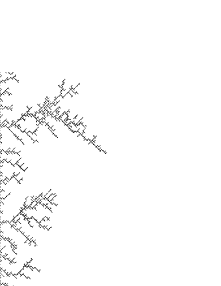
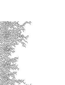
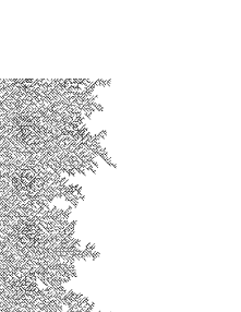
Figure 1: Snapshots of the invading fluid near breakthrough for the finite viscosity ratio case, using distinct types of oil and temperature differences. All patterns have been generated with the same distribution of permeability for the random links and $L=80$. From top to bottom, $B$ changes from 7 to 3, while from left to right, $\Delta T$ assumes the values -4, 0 and 4.

Here we assume that the viscosity of the fluid phases typically obey an exponential dependency on the inverse of temperature,

$$\mu_{o}=exp(B/T),$$ (3)

where the controlling physico-chemical parameter $B$, in units of temperature, is considered to be constant. One calls a fluid “heavy oil” if $B$ is high and “light oil” if $B$ is small. In order to impose a temperature gradient across the medium, different temperatures are assigned to the left (inlet) right (outlet) boundaries of the lattice and we consider, then, a linear temperature variation from inlet to outlet. This imposed gradient is constant in time, which is analogous to assume that the thermal conductivities of both fluids are negligible compared to that of the rock. The temperature difference is defined as $\Delta T=T_{inlet}-T_{outlet}$, and we carry out simulations many different dimensionless values of $T_{inlet}$ and $T_{outlet}$ ($T_{inlet}$, $T_{outlet}$ = 1, 2, 3, 4 and 5) such that -4 $\leq$ $\Delta T$ $\leq$ 4. Negative values of $\Delta T$ represent a cold injection which is not of technological interest, but can help to understand the nature beyond the fluid displacement under a temperature gradient. In this model, both link length, $\ell$, and reference temperature, $T_{r}$, are adjusting parameters which one can use to apply that model to a practical application. For example, if one considers $T_{r}=15^{\circ}C$ and $\ell=1$cm (size of the fraction of the rock which each link represent in the model), the temperature gradient varies from 0 to 75 ${}^{\circ}C/m$ as $\Delta T$ changes from 0 to 4. In the next section, we show results for the two different cases of the viscosity ratio. In both, $\mu_{o}$ is given by Eq. (3) while $\mu_{I}$ is constant, i.e., independent of the temperature. This can be justified since, for example, water, which is a typical invading fluid, has a viscosity that hardly changes, compared to many types of oils, for common operational temperature intervals.

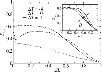
Figure 2: Near-breakthrough saturation of the invading fluid for the finite viscosity ratio case. The curves correspond to three values of the temperature difference, $\Delta T=-4$, $0$, and $4$, $B=5$ and $L=80$. In the inset, we also show the near-breakthrough saturation behavior, but for a fixed value of $\Delta T=4$, and $B=3$, $5$ and $7$.

III Results

In this section, we study the patterns of the invaded region and the percentage of recovered oil when an external fluid with unity viscosity is injected into the medium. According to our model, the viscosity ratio, $\mu_{o}/\mu_{I}$, has a finite value which changes on $x$-direction, if $\Delta T$ is different from zero. In Fig. 1 we show six different patterns of the invading fluid with the same distribution of random links for different values of $\Delta T$ and $B$. From top to bottom we change $B$ from $7$ to $3$, while from left to right $\Delta T$ assumes the corresponding values of $-4$, $0$ and $4$. We clearly observe that either decreasing $B$ or for positive values of $\Delta T$, the invading patterns become more compact.

In the isothermal case, $\Delta T=0$, the oil viscosity is a constant depending only on $B$. For a heavy oil ($B=7$), we can see finger patterns appearing in the invaded region. When $\Delta T>0$, the viscosity ratio is small on the left side of the lattice and becomes larger as the invading fluid penetrates in $x$-direction. First, the front advances compactly but at some time, a finger appears and grows faster until it reaches the other end of the lattice. In the opposite case, when $\Delta T$ $<$ 0, fingers appear initially and then become broader. For $B=3$, the changes in the viscosity ratio due to the temperature difference suppress the appearance of fingers.

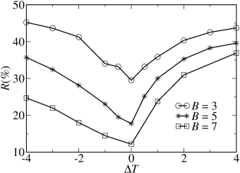
Figure 3: Percentage of recovered oil versus $\Delta T$ for the finite viscosity ratio case using three different values of $B$ and $L=80$.

For each set of parameters, we perform simulations with $50$ realizations of the disordered porous media, to obtain average values of both the invading fluid saturation and the percentage of recovered oil at the breakthrough. In Fig. 2, we show the near-breakthrough saturation profile of the invading fluid for different values of $\Delta T$ and $B$. We observe that for a positive $\Delta T$ the saturation profile has a plateau before it starts decreasing in the $x$-direction. However, for a negative $\Delta T$, finger patterns in the beginning of the lattice produce a dip in the saturation profile close to the inlet. The percentage of recovered oil versus $\Delta T$ is shown in Fig. 3 for three different values of $B$. We see that, despite heavy oil recovery is smaller, all types of oil tend to the recovery performance for high values of $\Delta T$.

Now, we study the recovery of an oil that is much heavier than the invading fluid, i.e., for the case of an extremely large viscosity ratio, $\mu_{o}/\mu_{I}\rightarrow\infty$. This idealized condition is implemented here by considering that the pressure in the invaded fluid immediately adjusts to the injection pressure, i.e., the invading fluid is inviscid. This simplification allows us to simulate bigger lattice sizes, since we need to solve Eqs. (2) only for non-invaded sites.

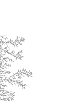
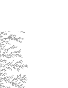
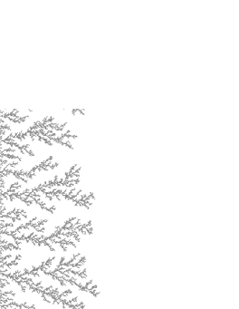
Figure 4: Snapshots of the invading fluid near breakthrough for the infinite viscosity ratio case. All patterns have been generated with the same distribution of permeability for the random links, $B=5$ and $L=256$. From left to right, $\Delta T=-4$, $0$ and $4$.

In this case, the observed patterns of the interface are always viscous fingering-like, as shown in Fig. 4, for $\Delta T=-4$, $0$ and $4$, with $B=5$ and $L=256$. For $\Delta T=0$, these patterns show fingers which agree with well know two-phase displacement patterns with infinite viscosity ratio homsy ; chen . We can also see that different patterns occur for different values of $\Delta T$. The reason for this behavior is that, despite the inviscid characteristic of the defending fluid, the oil viscosity has a finite value given by Eq. (3) which falls as the temperature is raised. Then the number of longer fingers for $B=5$ increases with $\Delta T$ as shown Fig. 4. This observation is also valid for $B=1$ and $3$ (not shown), and therefore represents a standard behavior in the case of infinite viscosity ratio.

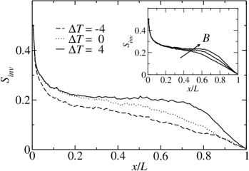
Figure 5: Near-breakthrough saturation of the invading fluid for the infinite viscosity ratio case. The curves correspond to three values of the temperature difference, $\Delta T=-4$, $0$, and $4$, $B=5$ and $L=256$. In the inset, we also show the near-breakthrough saturation behavior, but for a fixed value of $\Delta T=4$, and $B=1$, $3$ and $5$.

For each set of parameters, we averaged over 100 realizations to obtain the invading fluid saturation and the percentage of recovered oil. The near-breakthrough saturation profile of the invading fluid is shown in Fig. 5 for different values of the relevant parameters. For a negative value of $\Delta T$, the saturation profile always decays in $x$-direction. However, for a positive $\Delta T$, we can identify a region in the center of the medium with approximately constant saturation. The extension of this region increases with $B$ because heavier oils create slower and wider fingers, which tend to make the invasion patterns more compact.

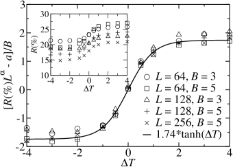
Figure 6: Percentage of recovered oil versus $\Delta T$ calculated in the infinite viscosity ratio case, for different values of $L$ and $B$. In the main plot, after proper rescaling, we show that these curves collapse on the top of each other and can be all fitted to a hyperbolic tangent function. In the inset, we show the same results before rescaling.

In the inset of Fig. 6, the percentage of recovered oil $R(\%)$ versus $\Delta T$ is shown for different values of $L$ and $B$. The main plot shows that, after rescaling, these curves collapse on the top of each other and can be closely described by a hyperbolic tangent function in the form,

$$R(\%)=\frac{a+bB\tanh(\Delta T)}{L^{\alpha}},$$ (4)

with parameters $a=51.11$ and $b=1.74$ obtained through the best nonlinear fit to the data. The exponent $\alpha$ is found to be about $0.2$ and can be computed as $\alpha=d-d_{f}$, where $d=2$ is the Euclidian dimension of the lattice and $d_{f}$ is the fractal dimension, which is found to be $1.8$ for our system. The results show that above a certain value of temperature difference, $\Delta T\approx 2$, no relevant change in $R(\%)$ is observable anymore for all types of oil. This means that a too strong temperature gradient can be an unnecessary cost to the recovery process.

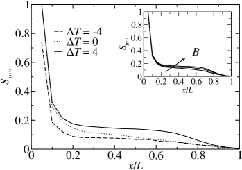
Figure 7: Near-breakthrough saturation profile of the invading fluid penetrating in a cubic lattice for the case of infinite viscosity ratio. The curves are the results of simulations for $\Delta T=-4$, $0$, and $4$, with parameter $B=5$, and system size $L=20$. In the inset, we also show the near-breakthrough saturation behavior, but for a fixed value of $\Delta T=4$, and $B=3$, $5$ and $7$.

Finally, we also performed simulations with our model in the infinite viscosity ratio regime using a more realistic three-dimensional porous medium substrate. More precisely, we obtained results for a cubic lattice with size $L=20$ and averaged over 100 realizations for several values of $B$ and $\Delta T$. As shown in Figs. 7 and 8, the saturation profiles and the recovery performance of the system, respectively, remain basically the same as compared to the results found for two-dimensional porous media models (for comparison, see Figures 5 and 6). This qualitative similarity reinforces the validity of our approach as a way to increase the efficiency of the recovery process by means of a temperature gradient.

IV Conclusions

In summary, the main purpose here was to investigate how the front between two immiscible fluids propagates in a model porous medium as a function of the ratio of their viscosity and under the influence of an imposed global temperature gradient. An obvious technological application of our study would be to enhance the recovery efficiency of oil being pushed by hot-water in a petroleum reservoir. In our simulations, this has been accomplished by explicitly coupling the oil viscosity with the inverse of temperature locally in terms of a simple exponential dependence. We thus proceeded with the displacement of several types of oil through many realizations of disordered porous medium, and subjected to a range of distinct temperature differences.

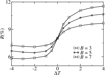
Figure 8: Dependence of the percentage of recovered oil on the temperature difference $\Delta T$ or different values of $B$ on a cubic lattice with $L$ = 20 for infinite viscosity ratio.

Two different regimes of viscosity ratio have been studied. In the first, oil viscosity changes with temperature and the viscosity ratio is always finite, but can vary over several orders of magnitude. In the second regime, oil is assumed to be “heavy”, in the sense that it is a extremely viscous when compared do the invading fluid, even if a maximum temperature difference is applied, hence the viscosity ratio can be considered as infinite. We find that the best conditions for recovery are significantly dependent on the adopted regime. In the finite viscosity ratio case, an oil with a viscosity that is only weakly dependent on the temperature is better recovered, independently on the strength or sign of the gradient. Also in this case, different invasion patterns can be observed as the viscosity ratio changes, namely, we find fronts that are compact, unstable and sometimes a mixing of both.

Differently, in the infinite viscosity ratio case, oil recovery increases with the exponential parameter $B$ if the temperature difference is positive. Moreover, recovery is found to follow a hyperbolic tangent behaviour on the temperature difference and the best recovery is obtained for positive temperature gradients (Hot-Water Injection). It would be interesting to verify our predictions with experimental results. Since field experiments in this area are usually difficult and expensive, it would be advisable to run laboratory-size experiments in which interface patterns are dynamically registered and the recovered volume is systematically measured while a viscous fluid is displaced by a less viscous one in a porous medium under the influence of temperature gradients.

- (1) M. Prats, Thermal Recovery (Monograph Series SPE of AIME, Richardson, 1982).
- (2) B. C. Craft and M. F. Hawkins, Applied Petroleum Reservoir engineering - second edition (Prentice Hall, New Jersey, 1991).
- (3) G. Moore, R. Mehta, and M. Ursenbach, J. of Canadian Petroleum Technology 41, n 8, 16 (2002).
- (4) A. T. Turta and A. K. Singhal, J. of Canadian Petroleum Technology 43, n 2, 29 (2004).
- (5) M. I. Kuhlman, SPE 86954 (2004).
- (6) J. S. Andrade, A. D. Araújo, S. V. Buldyrev, S. Havlin, and H. E. Stanley, Physical Review E 63, 051403 (2001).
- (7) M. Ferer, G. S. Bromhal, and D. H. Smith, Advances in Water Resources 30, 284 (2005).
- (8) M. Ferer, W. N. Sams, R. A. Geisbrecht, and D. H. Smith, Phys. Rev. E 47, 2713 (1993).
- (9) J. S. Andrade, M. P. Almeida, J. Mendes Filho, S. Havlin, B. Suki, and H. E. Stanley, Phys. Rev. Lett. 79, 3901 (1997).
- (10) P. R. King, J. S. Andrade, S. V. Buldyrev, N. Dokholyan, Y. Lee, S. Havlin, and H. E. Stanley, Physica A 266, 107 (1999).
- (11) H. Auradou, K. J. Måløy, J. Schmittbuhl, A. Hansen, and D. Bideau, Phys. Rev. E 60, 7224 (1999).
- (12) J. S. Andrade, U. M. S. Costa, M. P. Almeida, H. A. Makse, and H. E. Stanley, Phys. Rev. Lett. 82, 5249 (1999).
- (13) Y. Lee, J. S. Andrade, S. V. Buldyrev, N. V. Dokholyan, S. Havlin, P. R. King, G. Paul, and H. E. Stanley, Phys. Rev. E 60, 3425 (1999).
- (14) M. Sahimi, Rev. Mod. Phys. 65, 1393 (1993).
- (15) J. S. Andrade, S. V. Buldyrev, N. V. Dokholyan, S. Havlin, P. R. King, Y. Lee, G. Paul, and H. E. Stanley, Phys. Rev. E 62, 8270 (2000).
- (16) A. D. Araujo, W. B. Bastos, J. S. Andrade, and H. J. Herrmann, Phys. Rev. E 74, 010401(R) (2006).
- (17) R. Lenormand, E. Touboul, and C. Zarcone, J. Fluid Mechanics 189, 165 (1988).
- (18) A. D. Araujo, J. S. Andrade, and H. J. Herrmann, Phys. Rev. Lett. 97, 138001 (2006).
- (19) C. Lu and Y. C. Yortsos, American Insitute of Chemical Engineers 51, 1279 (2005).
- (20) C. A. Lu and Y. C. Yortsos, Phys. Rev. E 72, 036201 (2005).
- (21) C. Lu and Y. C. Yortsos, Industrial & Engineering Chemistry Research 43, 3008 (2004).
- (22) E. Aker, K. J. Måløy, A. Hansen, and G. G. Batrouni, Transp. in Porous Media 32, 163 (1998).
- (23) E. Aker, K. J. Måløy, and A. Hansen, Phys. Rev. E 58, 2217 (1998).
- (24) G. M. Homsy, Annu. Rev. Fluid Mech. 19, 271 (1987).
- (25) J.-D. Chen and D. Wilkinson, Phys. Rev. Lett. 55, 1892 (1985).
- (26) T. Ramstad, A. Hansen, and P.E. Øren, Phys. Rev. E 79, 036310 (2009).
- (27) M. Hashemi, B. Dabir, and M. Sahimi, AIChE J. 45, 1365 (1999).
- (28) H. A. Knudsen and A. Hansen, Eur. Phys. J. B 49, 109 (2006).