A FOSSIL BULGE GLOBULAR CLUSTER REVEALED BY VLT MULTI-CONJUGATE ADAPTIVE OPTICS

Abstract

The globular cluster HP 1 is projected on the bulge, very close to the Galactic center. The Multi-Conjugate Adaptive Optics (MCAO) Demonstrator (MAD) at the Very Large Telescope (VLT) allowed to acquire high resolution deep images that, combined with first epoch New Technology Telescope (NTT) data, enabled to derive accurate proper motions. The cluster and bulge field stellar contents were disentangled by means of this process, and produced unprecedented definition in the color-magnitude diagrams for this cluster. The metallicity of [Fe/H]$\approx$-1.0 from previous spectroscopic analysis is confirmed, which together with an extended blue horizontal branch, imply an age older than the halo average. Orbit reconstruction results suggest that HP 1 is spatially confined within the bulge.

1 Introduction

A deeper understanding of the globular cluster population in the Galactic bulge is becoming possible, thanks to high resolution spectroscopy and deep photometry, using 8-10m telescopes. An interesting class concerns moderately metal-poor globular clusters ([Fe/H]$\approx$-1.0), showing a blue horizontal branch (BHB). A dozen of these objects are found projected on the bulge (Barbuy et al., 2009), and they might represent the oldest globular clusters formed in the Galaxy.

According to Gao et al. (2010), the first generation of massive, fast-evolving stars, formed at redshifts as high as z$\approx$35. Second generation low mass stars would be found primarily in the inner parts of the Galaxy today, as well as inside satellite galaxies. Nakasato & Nomoto (2003) suggest that the metal-poor component of the Galactic bulge should have formed through a subgalactic clump merger process in the proto-Galaxy, where star formation would be induced and chemical enrichment by supernovae type II occurred. The metal-rich component instead would have formed gradually in the inner disk. Therefore, metal-poor inner bulge globular clusters might be relics of an early generation of long-lived stars formed in the proto-Galaxy.

Another aspect of the interest of inner bulge studies, comes from evidences that stellar populations in the Galactic bulge are similar to those in spiral bulges and elliptical galaxies, and therefore they are of great interest as templates for the study of external galaxies (Bica, 1988; Rich, 1988). In the past, the detailed study of the bulge globular clusters was hampered by high reddening and crowding. With the improvement of instrumentation, it is now possible to derive accurate proper motions, and to apply membership cleaning. Most previous efforts in the direction of proper motion studies were carried out using Hubble Space Telescope - HST data by our group (e.g. (Zoccali et al., 2001)) for NGC 6553, or Feltzing & Johnson (2002) for NGC 6528, and Kuijken & Rich (2002) for field stars, among others.

In a systematic study of bulge globular clusters (e.g. Barbuy et al. (1998, 2009), we identified a sample of moderately metal-poor clusters ([Fe/H]$\sim$-1.0) concentrated close to the Galactic center. HP 1 has a relatively low reddening, and appeared to us as a suitable target to be explored in detail in terms of proper motions. Its coordinates are $\alpha=17^{\rm h}31^{\rm m}05.2^{\rm s}$, $\delta=-29^{\rm o}58^{\prime}54^{\prime\prime}$ (J2000), and projected at only 3.33^∘ from the Galactic center (l=-2${}^{\circ}.5748$, b=$2^{\circ}.1151$).

In 2008, the European Southern Observatory (ESO) announced a public call for Science Verification of the Multi-Conjugate Adaptive Optics Demonstrator (MAD, Marchetti et al. (2007)), installed at the ESO UT3-Melipal telescope. Several star clusters were observed with the MAD facility, delivering high quality data for the open clusters Trapezium, FSR 1415 and Trumpler 15 (Bouy et al., 2008; Momany et al., 2008; Sana et al., 2010), the globular clusters Terzan 5 and NGC 3201 (Ferraro et al., 2009; Bono et al., 2010), and 30 Doradus (Campbell et al., 2010). The major advantage of MAD is that it allows correcting for atmospheric turbulence over a wide $2^{\prime}$ diameter field of view, and as such, constitutes a pathfinder experiment for future facilities at the European Extremely Large Telescope (E-ELT). Wide field adaptive optics with large telescopes opens a new frontier in determining accurate parameters for most globular clusters, that remain essentially unstudied because of high reddening, crowding (cluster and/or field), and large distances.

In Sect. 2 the observations and data reductions are described. In Sect. 3 the HP 1 proper motions are derived. The impact of the high quality proper motion cleaned Color-Magnitude Diagrams (CMDs) on cluster properties are examined in Sect. 4. The cluster orbit in the Galaxy is reconstructed in Sect. 5. Finally, conclusions are given in Sect. 6.

2 Observations and Data Analysis

MAD was developed by the ESO Adaptive Optics Department to be used as a visitor instrument at VLT-Melipal in view of an application to the E-ELT. It was installed at the visitor Nasmyth focus and the concept of multiple reference stars for layer oriented adaptive optics corrections was introduced. This allows a much wider and more uniform corrected field of view, providing larger average Strehl ratios and making the system a powerful diffraction limit imager. This is particularly important in crowded fields where photometric accuracy is needed. Following our successful use of MAD in the first Science Demonstration (Momany et al. 2008), we were granted time to observe HP 1 in the second Science Demonstration ().

HP 1 was observed on August $15^{th}$, 2008. Table 1 displays the log of the $J$ and $K_{\rm s}$ (for brevity we use $K$) observations. Clearly, the seeing in $K$ was excellent being almost half that in $J$ ($0\farcs 23$ $vs$ $0\farcs 38$). The MAD infrared scientific imaging camera is based on a $2048\times~{}2048$ pixel HAWAII-2 infrared detector with a pixel scale of $0\farcs 028$. In total, $25$ min. of scientific exposures were dedicated to each filter, and subdivided into $5$ dithered images.

The images were dark and sky-subtracted and then flat-fielded following the standard near infrared recipes (e.g. Momany et al. 2003), within iraf environment. The typical dithering pattern of a MAD observation allows a field of view of $\sim 2^{\prime}$ in diameter. Within this field of view, three reference bright stars ($R$ magnitudes that ranged between $12.5$ and $13.8$ according to their UCAC2 magnitude system) were selected to ensure the optics correction. However, one of these proved to be a blend of two stars, which did not allow a full optical correction of the field.

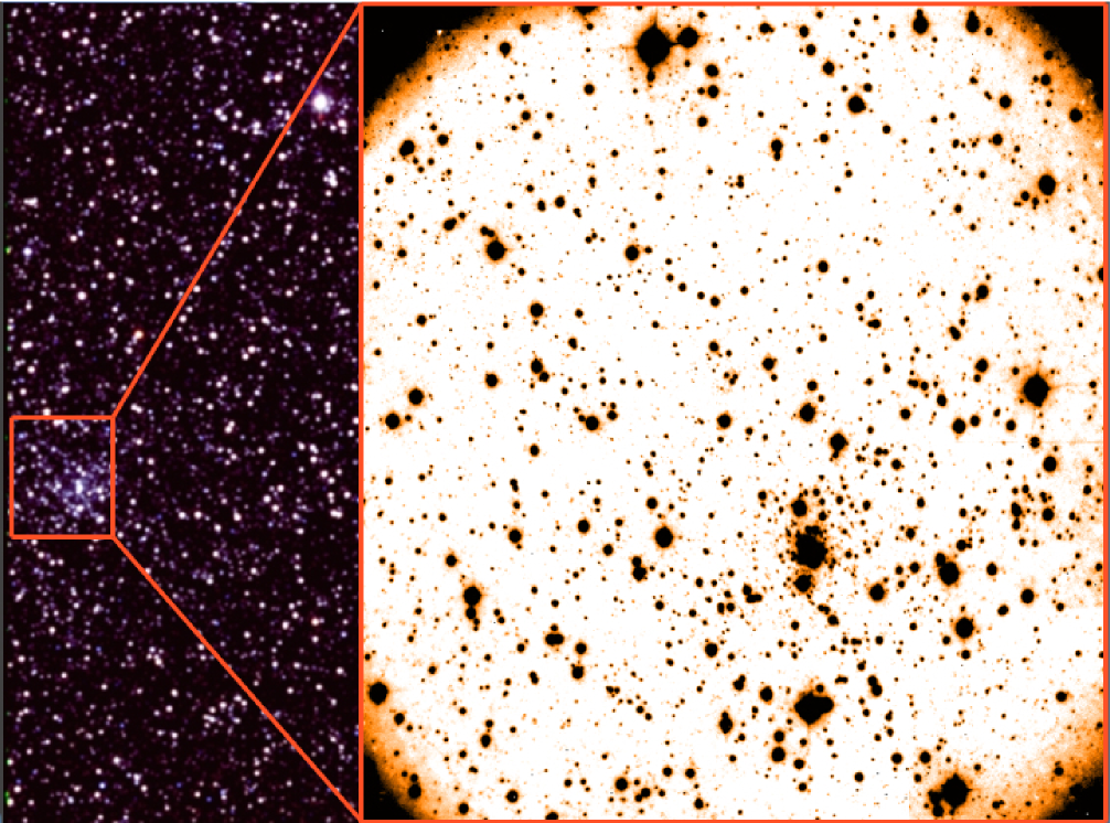
Figure 1: MAD image of the globular cluster HP 1, obtained at the ESO-VLT at Paranal, Chile. Left panel is a composite color image of HP 1 from the near-infrared 2MASS survey; Right panel is a close-up of the MAD $K$-band image covering the central $1\farcm 8\times 1\farcm 8$ of HP 1. North is up, East to the left.

Figure 1 shows the mosaic of all 10 $J$ and $K$ images as constructed by the daophot/montage2 task. The superb VLT/MAD resolution is illustrated when compared to that seen in the 2MASS $K$ image of HP 1. For the proper motion purposes, the MAD data set represents our second epoch data. The displacement of the HP 1 stellar content was derived by comparing the position of the stars in this data set with respect to that of SUSI@NTT obtained on May $16^{th}$, 1994 (Ortolani et al., 1997). The epoch separation is $14.25$ years. It is worth emphasizing that the seeing of 0.45” for the V image of HP 1 is one of the best obtained at the NTT (Ortolani et al., 1994, 1997).

The photometric reductions of the two data sets (NTT and MAD) were carried out separately. We found about 3100 stars in common between the MAD and NTT data, which were used for the proper motion analyses.

2.1 Photometric Reduction and Calibration

The stellar photometry and astrometry were obtained by point spread function (PSF) fitting using daophot ii/allframe (Stetson et al., 1994). Once the FIND and PHOT tasks were performed and the stellar-like sources were detected, we searched for isolated stars to build the PSF, for each single image. The final PSF was generated with a PENNY function that had a quadratic dependence on frame position. ALLFRAME combines PSF photometry carried out on the individual images and allows the creation of a master list by combining images from different filters. Thereby this pushes the detection limit to fainter magnitudes and provides a better determination of the stellar magnitudes (given that 5 measurements were used for each detected star).

Our observing strategy employed the same exposure time for all images, and no bright red giant stars were saturated. When producing the photometric catalog in one filter (and since only the central part of the field of view had multiple measurements of any star), stars appearing in any single image were considered to be real. Later, when producing the final $JK$ color catalog, only those appearing in both filters were recorded (this way we removed essentially all detections due to cosmic rays and other spurious detections). The photometric catalog was finally transformed into coordinates with astrometric precision by using 12 UCAC2 reference stars with $R\leq 16.2$.

Photometric calibration of the $J$ and $K$ data has been made possible by direct comparison of the brightest MAD non-saturated ($8.0\leq~{}K\leq 13.0$) stars with their 2MASS counterpart photometry.

From these stars we estimate a mean offset of $\Delta~{}J_{\rm J@MAD-J@2MASS}=-3.157\pm 0.120$ and $\Delta~{}K_{\rm K@MAD-K@2MASS}=-1.395\pm 0.134$.

Photometric errors and completeness were estimated from artificial star experiments previously applied to similar MAD data (Momany et al. 2008).

The images with added artificial stars were re-processed in the same manner as the original images. The results for photometric completeness showed that we reach a photometric completeness of $\sim 75\%,50\%$ and $10\%$ around $K\simeq 17.0,17.5$ and $\sim 18.0$, respectively.

3 Derivation of the proper motions

The proper motion of the HP 1 stellar content was derived by estimating the displacement in the ($x,y$) instrumental coordinates between MAD (second epoch data) and the NTT (first epoch) data. Since this measurement was made with respect to reference stars that are cluster members, the motion zero point is the centroid motion of the cluster. The small MAD field of view is fully sampled by the wider NTT coverage, and thus essentially all MAD entries had NTT counterparts for proper motion determination. In this regard, we note that the photometric completeness of the MAD data set is less than that of the optical $V,I$ NTT data, that reached at least 2 magnitudes below the cluster turnoff (Ortolani et al., 1997).

The daophot/daomaster task was used to match the photometric MAD and NTT catalogs, using their respective ($x,y$) instrumental coordinates. This task employed a cubic transformation function, which, with a matching radius of $0.5$ pixels or $0\farcs 015$, easily identified reference stars among the cluster’s stars (having similar proper motions). As a consequence, the stars that matched between the 2 catalogs were basically only HP 1 stars. In a separate procedure, the J2000 MAD and NTT catalogs transformed into astrometric coordinates, were applied to a matching procedure, using the iraf/tmatch task. This first/second epoch merged file included also the ($x,y$) instrumental coordinates of each catalog. Thus, applying the cubic transformation to both coordinate systems yielded the displacement with respect to the centroid motion of HP 1. An extraction within a $1.5$ pixel radius around ($0,0$) in pixel displacement showed to contain most, and essentially only HP 1 stars, and we will use this selection for the rest of the paper.

On the other hand, stars outside this radius (i.e. representing the bulge populations) are more dispersed, and required a careful analysis. In a first attempt we used only the stars with $\Delta$y $<$ -1 (in order to avoid cluster stars) to get the baricentric position of the field bulge population in x, and stars with $\Delta$ x $>$ 1 to measure the field bulge population in y. After a number of tests with different selections, in a second attempt we made a two gaussian component fit along a 0.2 pixels wide strip connecting the center of the cluster distribution and the field distribution. For the present analysis we adopted for the proper motion of the cluster, relatively to the field, the mean of the two determinations ($\Delta$ x, $\Delta$ y) = (-2.1, 1.96). From the gaussian fit we derived the width of the distributions of the cluster and field stars, resulting respectively $\sigma$=0.583 and 2.565 pixels, corresponding to 15 and 41 mas respectively. This is the error of the single star position. The statistical error of the mean is obtained by dividing the single star error by the square-root of the number of stars used (about 1700 in the cluster and 1500 in the bulge) for each of the two measurements. The error on the mean position of the field obviously dominates and corresponds to about 0.05 pixels, or 1.3 mas (about 0.1 mas/year). This is indeed a very small error. We performed a number of tests fitting the cluster stars and the field stars in different conditions checking for additional uncertainties. A further quantitative evaluation of the fitting uncertainty can be obtained measuring the different distances between the centers of the HP1 proper motions cloud to that of the field, propagated from the error on the angle of the line connecting the two groups of stars. The angle of the vector joining the center of the HP1 proper motion cloud to that of each star of the bulge was computed, and a Gaussian fit was performed which returned a 1-sigma dispersion of 14^∘. This uncertainty propagates on the distances of the two groups by about 0.39 mas/year, dominating over the other discussed sources.

3.1 Astrometric errors

The astrometric errors are the combination of different random and systematic errors (Anderson et al., 2006). They concluded that in the case of relative ground-based astrometry in a small rich field, the main error sources are random centering errors due to noise and blends, and random-systematic errors due to field distorsions, and finally by systematic errors due to chromatic effects.

i) Centering errors: Considering that we used two very different data sets, a first epoch based on direct CCD photometry, and a second one, on the corrected infrared adaptive optics (with a much wider scale and better resolution), we can assume that the astrometric random errors are dominated by the first epoch classical CCD photometry. Following Anderson et al. (2006), we performed a test with 3 consecutive NTT images of Baade’s Window taken in the same night. They were obtained with equal (4 min.) exposure times, and nearly at the same pixel positions. The seeing was stable and these images were obtained about 1 hour later than the 10 min. cluster V exposure.

This Baade’s Window field was chosen because the stars are uniformly distributed across the image, and the density of stars is similar to the HP 1 field. These images were analysed in Ortolani et al. (1995). The position of the stars in common were compared. The photometric and astrometric errors are shown in Figs. 2. The astrometric centering error, averaged over the whole dynamic range, is 0.1 pixels, as indicated in Fig. 2. This corresponds to 13 mas, which is comparable with the 7 mas pointing error by Anderson et al. (2006). The value of 13 mas amounts to 0.91 mas/yr in an interval of 14.25 yr. Taking into account the number of about 3000 stars (half field and half cluster) used for the proper motion derivation of HP 1, this leads to a minor error of 0.022 mas.

ii) Field distortion errors: The field distortion analysis is usually performed employing shifted images of a field with uniformly distributed stars. HP 1 multiple shifted images are not available in our first epoch run. To estimate the distortions, we compared the proper motion of cluster stars in HP 1 NTT images as a function of the distance from the optical center. The distribution did not show any relevant trend, and the statistical analysis indicates that there is no significant shift above 0.01 pixel across the field. This corresponds to 0.19 mas/yr.

iii) Chromatic errors: Chromatic errors are due to the different refraction, both atmospheric and instrumental, on stars with different colors. The refraction dependence on wavelength (inverse quadratic to first approximation) makes this effect more pronounced in V, I than in the near infrared.

Ideally, a chromatic experiment should include a measurement of the displacement of stars with different colors, at different airmasses. However, we do not have specific observations for this test. Thus, we followed the procedure given by Anderson et al. (2006) where they measured the displacement of stars as a function of their colors. We took the resulting pixel displacement of the cluster stars, and separately checked the shift variations with the color (V-I). Such plot does not show an evident dependence on color. This is expected since our NTT observations were taken very close to the zenith (airmass$\sim$1.04), and the infrared MAD data have a negligible effect.

In order to further quantify any chromatic systematic effect, we subdivided the sample of cluster stars into a redder (V-I $>$ 2.2) and a bluer (V-I $<$ 2.2) groups, of 106 and 171 stars respectively. The displacement between the two groups resulted to be 0.031$\pm$0.03 pixels, corresponding to 0.9 mas. In 14.25 yr, this gives 0.06 mas/yr.

iv) Total errors:

By quadratically adding the errors on centering, distortion and chromatic effects of respectively 0.022 mas/yr, 0.19 mas/yr, and 0.06 mas/yr, a total contribution of these errors of 0.2 mas/yr is obtained.

The estimated error of 0.39 mas/yr in the proper motion value indicates that the effect due to the mutual field and cluster stars contamination dominates over the astrometric pointing, distortion and chromatic errors.

4 The proper motion cleaned Color-Magnitude Diagram of HP 1

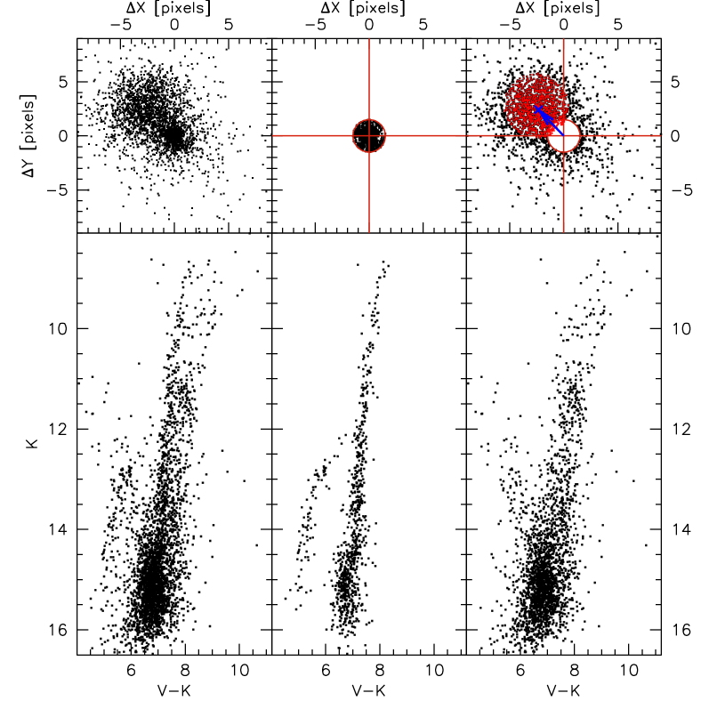
Figure 3: HP 1: Proper motion decontaminated $K$ $vs.$ $J-K$ CMD. Upper panels: Left: Displacement of NTT (1st epoch) - MAD (2nd epoch), plotted in MAD pixel scale; Middle: Cluster sample is encircled where $l$, $b$ directions are indicated by the arrows; Right: Field sample only. Lower panels: Left: Observed CMD; Middle: Proper motion decontaminated cluster CMD. The two stars indicated as red squares are the two giant stars analysed with high resolution spectroscopy; Right: Remaining field stars CMD. The extraction is within a $1.5$ pixel radius.

Figure 3 presents the MAD $K$ $vs.$ $J-K$ CMDs showing the proper motion decontamination process in three panels: for the whole field, cluster proper motion decontaminated, and remaining field only. In the top panels are shown the displacements of stars between the NTT and MAD images, plotted in the MAD pixel scale.

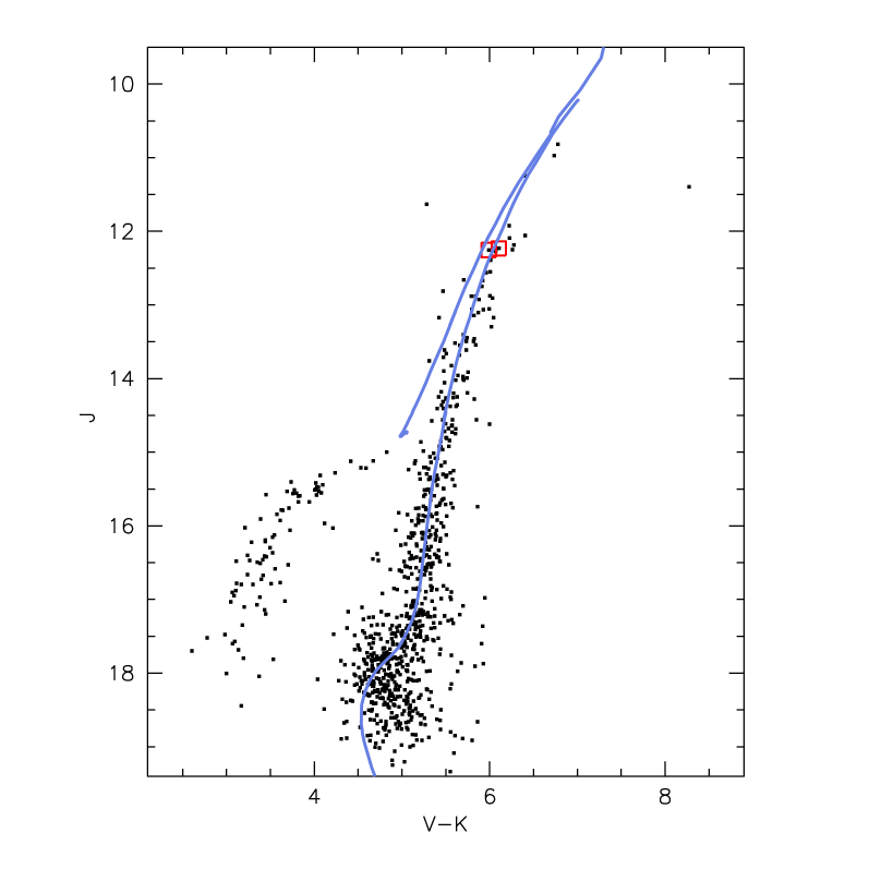
Figure 4: HP 1: $J$ $vs.$ $V-K$ CMD, built from a proper motion selected subsample of stars. The extraction is within a $1.5$ pixel radius, in pixel displacement. Padova isochrone of $Z=0.002$ and age of $13.7$ Gyr is overplotted on the observed CMD. A distance modulus of (m-M)_J = 15.3 and a reddening E(V-K) = 3.3 were adopted. The metallicity, distance, and reddening adopted for the fit are in agreement with the spectroscopic analysis (Barbuy et al. 2006). The present MAD photometry reaches the turn-off limit.

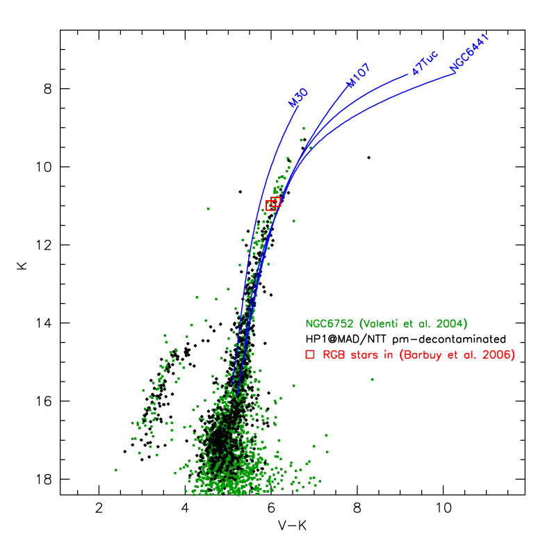
Figure 5: The $K$ $vs.$ $V-K$ HP 1 diagram (black dots) as compared with the NGC 6752 (green dots) catalog (Valenti et al. 2004). We assumed the fiducial values $(m-M)_{0}=13.18$, $E(B-V)=0.04$, $Av=3.1$, $Ak=0.38$. Also plotted are the red giant branches of comparison Galactic globular clusters (blue lines): M 30, M 107, 47 Tuc and NGC 6441 ([Fe/H]$-2.12,-1.04,-0.76$ and $-0.68$ (where the catalog and the red giant fiducials are from Valenti et al. 2004). The HP 1 bright red giants are clearly overlapping the M 107 fiducial (reflecting their similar metallicity) and are redder with respect to the NGC 6752 bright giants.

The decontaminated cluster CMD provides fundamental parameters to study its properties, in particular metallicity and age. Figure 4 shows a $J$ $vs.$ $V-K$ proper motion decontaminated CMD of HP 1. A distance modulus of (m-M)_J = 15.3 and a reddening of E(V-K) = 3.3 were applied, and a Padova isochrone (Marigo et al., 2008) with metallicity $Z=0.002$ and age of $13.7$ Gyr is overplotted. The fit confirms the cluster metallicity of [Fe/H]$=-1.0$, found from high resolution spectroscopy (Barbuy et al., 2006). We note that the turnoff is not as well matched as the giant branch, due to two well-known main reasons: the bluer turnoff in isochrones relative to observations is possibly connected with color transformations, and on the other hand, systematic bias in the photometric errors give brighter magnitudes close to the limit of the photometry. Similarly, Fig. 5 displays the $K$ $vs.$ $V-K$ HP 1 diagram as compared with the NGC 6752 ([Fe/H]$=-1.42$) mean locus (Valenti et al., 2004). The red giant branches of M 30, M 107, 47 Tuc and NGC 6441 of metallicities [Fe/H]$=-1.91,-0.87,-0.70$, and $-0.68$, respectively, are also overplotted, where the metallicity values, mean loci and the red giant fiducials are from Valenti et al. (2004). The HP 1 bright red giants clearly overlap the M 107 fiducial (reflecting their similar metallicity) and are redder with respect to the NGC 6752 bright giants. On the other hand, the cluster old age is reflected by the presence of a well defined and extended BHB (very similar to NGC 6752). Five RR Lyrae candidates appear in the RR Lyrae gap, at $4.2\leq~{}(V-K)\leq 5.0$. (Terzan, 1964a, b, 1965, 1966) reported 15 variable stars in HP 1, but none has been identified as RR Lyrae. The Horizontal Branch (HB) morphology is sensitive mainly to metallicity and age. The age effect is related to the so-called second parameter effect (Sandage & Wildey, 1967), as well demonstrated in models by Lee et al. (1994), Rey et al. (2001) and in observations by Dotter et al. (2010). In particular, Dotter et al. (2010) analysed the HB morphology from ACS/HST observations, based on the difference between the average HB $V-I$ color and the subgiant branch (SGB) color $\Delta~{}V-I^{SGB}_{HB}$, and concluded that age dominates the second parameter. This indicator is very sensitive to the cluster age, and more so around the metallicity $Z=0.002$.

For HP 1 the mean $V-I$ color difference between the SGB and the HB is $\Delta~{}V-I^{SGB}_{HB}=0.75\pm 0.01$. A comparison with Dotter et al. (2010)‘s sample shows that HP 1 has a very blue HB for its metallicity. We selected 5 clusters with the same HB morphological index, and found an average metallicity of [Fe/H]$=-1.9\pm 0.36$, and another group of 5 clusters, with a comparable metallicity to HP 1. This second group has an average $\Delta~{}V-I=0.46\pm 0.27$ which is considerably smaller than in HP 1, consistent with HP 1 having a much bluer HB. Both cluster groups have a mean age of $12.7\pm 0.4$ Gyr. From Fig. 17 of Dotter et al., we get an age difference of about 1 Gyr older for HP 1 relative to their sample of halo clusters with $\sim$12.7 Gyr, resulting for HP 1 an age of $\sim 13.7$ Gyr. Therefore HP 1 appears to be among the oldest globular clusters in the Galaxy.

For the distance determination, there are basically two methods: a) the relative distance between the cluster and bulk of the bulge field, and b) based on the absolute distance, which requires reddening values. For the first of these methods, we rely on the difference between the HP 1 horizontal branch at the RR Lyrae level, at $V=18.7$, and that of the bulge field at $V=19.35$. Thus the cluster is $\Delta~{}V=0.66$ brighter than the field, and taking into account metallicity effects on the HB luminosity ( (Buonanno et al., 1989), we obtain $\Delta~{}V=0.35\pm 0.14$. This implies that the cluster is 1.2$\pm$0.4 kpc in the foreground of the bulge bulk population. The uncertainty is due to the metallicity difference of about 1 dex between the bulge ([Fe/H]$\approx$0.0) and HP 1 ([Fe/H]$\approx$-1.0). Assuming the distance of the Galactic center to be R_GC=8.0$\pm$0.6 (Majaess et al., 2009; Vanhollebeke et al., 2009), a distance of d${}_{\odot}=6.8$ kpc is obtained. If the orbits of stars near the super massive black hole near the Galactic center method is used, a distance of R_GC=8.33$\pm$0.35 kpc is given by Gillessen et al. (2009). In this case the distance of HP 1 to the Sun is d${}_{\odot}=7.1$ kpc. This relative distance method is reddening independent, because the reddening of cluster and surrounding field is expected to be the essentially the same, due to a negligible reddening inside the bulge (Barbuy et al. 1998). Therefore the distance of the cluster to the Galactic center depends only on the assumed distance of the Galactic center.

The second method of absolute distances requires reddening determinations. From the optical and infrared CMDs, and adopting the absolute-to-selective absorption R${}_{\rm V}=3.2$ (Barbuy et al., 1998), we obtain a mean distance from the Sun of d${}_{\odot}=7.3\pm 0.5$ kpc. Within the uncertainties for the cluster and Galactic center distances, we conclude that HP 1 is probably the globular cluster located closest to the Galactic center.

For simplicity we assume the distance of HP 1 from the Sun to be d${}_{\odot}=6.8$ kpc hereafter.

5 Spatial motion of HP 1 in the Galaxy

5.1 Absolute proper motion

To compute the velocity components of HP 1’s motion we need its radial velocity and the proper motion. The heliocentric radial velocity v${}_{{\rm r}}^{{\rm hel.}}=45.8\pm 0.7$ km s^-1 was adopted from the high resolution analysis by Barbuy et al. (2006). The proper motion can be computed with respect to the bulge, and the bulge proper motion can then be subtracted. The bulge proper motion is a composition of the bulge internal kinematics, and the reflected motion of the LSR. Near the position of HP 1, the bulge kinematics is close to that of a rotating solid body with spin axis orthogonal to the Galactic plane (e.g., (Zhao, 1996)). Note also that this correction is not large: HP 1 is projected so close to the Galactic center that the rotational velocity of the bulge is closely aligned with the line of sight, so its tangential component is very small. Because both motions are parallel to the Galactic plane, it is convenient to work in Galactic coordinates.

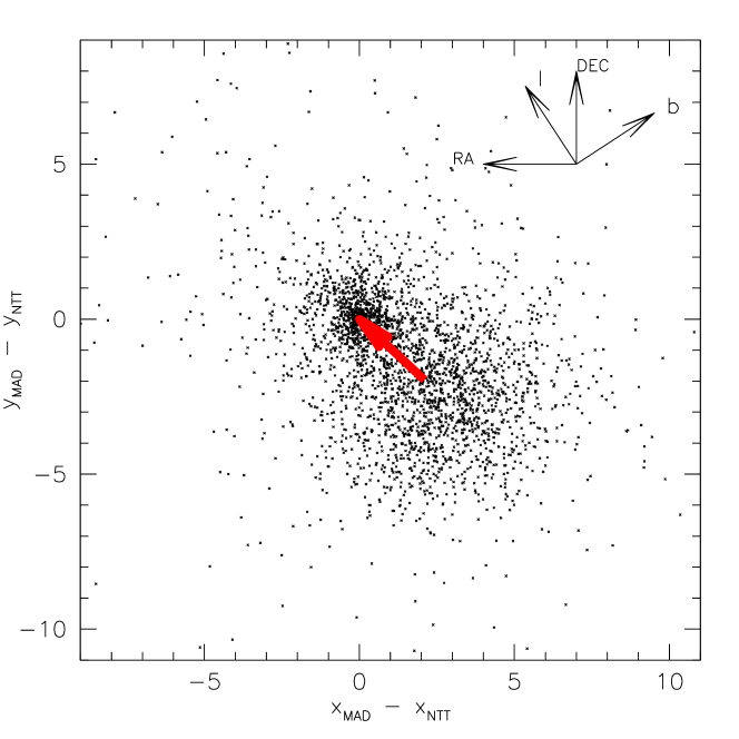
Figure 6: In the reference system $(\Delta x,\Delta y)=(x_{{\rm MAD}}-x_{{\rm NTT}},y_{{\rm MAD}}-y_{{\rm NTT}})$ with origin in HP1 the bulge has coordinates $(2.10,-1.96)$. Therefore the HP1 motion with respect to the bulge has a vector $\overrightarrow{u_{{\rm px}}}=(-2.10,1.96)$ (red arrow). Because RA and $\Delta x$ have opposite directions, the vector expressed in Equatorial coordinates is $\overrightarrow{u_{{\rm Eq}}}=(0\farcs 0588,0\farcs 05488)$. The relative orientation of the Equatorial and Galactic coordinate systems is shown in the upper right corner, making clear that the proper motion of HP1 is mostly along positive $l$, with a small component along negative $b$. The orbit must then be confined near the Galactic plane.

As Fig. 6 shows, the HP1 motion with respect to the bulge has a vector $\overrightarrow{u_{{\rm px}}}=(-2.10\,\-{\rm px},\-1.96\-\,{\rm px})$

To estimate the bulge internal motion, we note that Tiede et al. (1999) obtained a rotational velocity of $\sim 75\,\rm km~{}s^{-1}$, in their fields 6/05 and 6/18 (b=-6^∘ and field number), at positions $l=-8^{\circ}.7$ and $l=8^{\circ}.4$, respectively. In the solid body approximation, $v_{{\rm rot}}$ depends linearly on the radius $r$ (confirmed by Howard et al. (2008)), and at the position of HP1 (Sect. 1) we expect $v_{{\rm rot}}\simeq 75\rm km~{}s^{-1}/8.5^{\circ}\times 2^{\circ}.58=22.8$ km sec^-1 (where we assumed $l\propto r$ for small values of $l$). Basically the same value ($22.7\,\rm km~{}s^{-1}$) is predicted at a distance of $0.38\,{\rm kpc}$ ($=r_{\odot}\times\sin 2^{\circ}.58$ with $r_{\odot}=8.4\,{\rm kpc}$) by the angular velocity of $60.0\,\rm km~{}s^{-1}\,{\rm kpc}^{-1}$ adopted in our model (Sect. 5.2). Assuming that bulge stars are at the distance of the Galactic Center, the tangential component of $v_{{\rm rot}}$ is $v_{{\rm T}}=22.8\rm km~{}s^{-1}\times\sin 2^{\circ}.58/\cos 2^{\circ}.58=1.03$ km s^-1 directed toward increasing $l$. After adding $v_{{\rm T}}$ to $V_{{\rm LSR}}$, the composite motion of the bulge becomes $(\mu_{l},\mu_{b})_{{\rm bulge+LSR}}=(6.127,0)\,\rm mas~{}yr^{-1}$, and subtracting it from the relative motion quoted above yields for HP 1 $\mu_{l}\times\cos b=-0.65\pm 0.39\,\rm mas~{}yr^{-1}$ and $\mu_{b}=-1.34\pm 0.39\,\rm mas~{}yr^{-1}$. Using this proper motion, in the next section we calculate the cluster orbit.

5.2 HP 1 orbit in the Galaxy

The orbit was computed both with the axisymmetric model by Allen & Santillan (1991) and with a model including a bar. The models and integration algorithm are described in Jilkova et al. (in preparation). Similar models have also been used in Magrini et al. (2010). Compared to these earlier versions, the axisymmetric model was rescaled to match the more recent values of rotation velocity, solar Galactocentric distance and solar velocity relative to the LSR. Reid et al. (2009) estimated a rotation velocity of $254\pm 16\,\rm km~{}s^{-1}$, and a distance of $8.4\pm 0.6$ kpc, using the solar motion relative to the LSR determined by Dehnen & Binney (1998). However, the analysis of Dehnen et al. was recently re-examined by Schönrich et al. (2010) obtaining slightly different values – the component in the direction of solar Galactic rotation is $7\,\rm km~{}s^{-1}$ higher. Taking this into account, we rescaled the Allen & Santillan (1991) parameters to get values of $243\,\rm km~{}s^{-1}$ at $8.4$ kpc, which is also consistent with the results of Reid & Brunthaler (2004) who obtained the solar rotation velocity from the proper motion of Sgr A*.

The Galactic bar is modeled by a Ferrers potential of an inhomogeneous triaxial ellipsoid (Pfenniger, 1984). The model parameters are adopted from Pichardo et al. (2004) with length of 3.14 kpc, axis ratio 10:3.75:2.56, mass of $0.98\times 10^{10}$ M_⊙, angular velocity of $60.0\,\rm km~{}s^{-1}\,{\rm kpc}^{-1}$, and an initial angle with respect to the direction to the Sun of $20^{\circ}$ (in the direction of Galactic rotation). For the axisymmetric background we keep the potential described above with decreased bulge mass by the mass of the bar.

The initial conditions for the orbit calculations are obtained from the observational data characterizing the cluster: coordinates, distance to the Sun, radial velocity, and proper motion. To evaluate the impact of the measurement errors, we calculate a set of $1,000$ orbits with initial conditions given by sampling the distributions of observational inputs. We assume normal distributions for the distance to the Sun, radial velocity, and proper motion. The errors on radial velocity and proper motion components are given above, while for the distance to the Sun we assumed an error of $10\%$.

The transformation of the observational data to the Cartesian coordinate system centered on the Sun was carried out with the Johnson & Soderblom (1987) algorithm. The velocity vector with respect to the LSR is then obtained by correction for the solar motion with respect to the LSR from Schönrich et al. (2010): $(U,V,W)_{\odot}=(11.1,12.24,7.25)\,\rm km~{}s^{-1}$ (right-handed system, with $U$ in the direction to the Galactic center and $V$ in the Galactic rotation direction). The final transformation to the Galactocentric coordinate system was made by using the solar Galactocentric distance 8.4 kpc and the LSR rotation velocity of $243\,{\rm\rm km~{}s^{-1}}$ (see above). We obtain proper motions in equatorial coordinates $\mu_{{\rm RA}}\times\cos{\rm DEC}=0.76\pm 0.39\,{\rm mas}\,{\rm yr^{-1}}$, $\mu_{{\rm DEC}}=-1.28\pm 0.39\,{\rm mas}\,{\rm yr^{-1}}$, and Cartesian coordinates and velocities $(x,y,z)=(1.59,0.31,0.25)\,{\rm kpc}$ and $(v_{x},v_{y},v_{z})=(-57.47,-231.99,-34.26)\,\rm km~{}s^{-1}$. We adopted a right-handed, Galactocentric Cartesian system ($x$ to the Sun direction, $z$ to the north galactic pole).

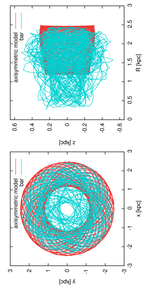
Figure 7: Galactic orbit of the cluster: projections into the Galactic and meridional plane are plotted on the left and right, respectively. Orbit in axisymmetric model is plotted by red line, orbit in the model including bar by blue line. The initial conditions are given by mean observational input data. See text for detailed description of integrations.

We integrate the orbits with such initial conditions backwards for an interval of $3$ Gyr using a Bulirsch-Stoer integrator with adaptive time-step (Press et al., 1992). The example of orbits given by the average values of the observational data is given in Fig. 7. The presence of the bar disturbs the orbit of this central globular cluster, causing deviations not found in the axisymmetric model. This can be considered as an upper limit for the excursions that the cluster can make inward and outward. Even so, it is clear that the cluster is essentially confined within the bulge.

Running simulations for a longer time is not very meaningful because there is evidence that the bar structure is a transient feature. For example Minchev et al. (2010) suggest that the current bar might have formed only $2$ Gyr ago. It is then impossible to simulate the orbit along the entire life of the Milky Way, but one can guess that older bars would have had a similar effect on the orbit of HP1. Note that we also included the spiral arms, but they do not change the orbit significantly. They are very weak and the orbit is too close to the Galactic center to be influenced by any radial migration due to bar and spiral arm interaction.

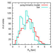
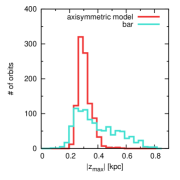
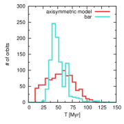
Figure 8: Distributions of orbital parameters: apogalacticon $R_{\mathrm{a}}$, vertical height of orbit $|z_{\mathrm{max}}|$, and phase period $T$. Distributions given by the axisymmetric model are plotted by red line and in the model with bar by blue line (same as in Fig. 7).

We calculated orbital parameters as averaged values over individual revolutions in the Galactic plane for each orbit. Distributions for apogalacticon $R_{\mathrm{a}}$, vertical height of orbit $|z_{\mathrm{max}}|$, and phase period $T$ are shown in Fig. 8. In general the orbits do not reach galactic distances larger than 5 kpc and also the cluster remains close to the Galactic plane ($|z_{\mathrm{max}}|<0.3$ kpc for the axisymmetric model, $|z_{\mathrm{max}}|<0.6$ kpc for the model including bar).

For comparison purposes, we also computed the HP 1 orbit using the code developed by Mirabel et al. (2001), that includes the Galactic spheroidal and the disk potentials. It was recently applied to $\omega$ Centauri orbital simulations (Salerno et al., 2009). In this method we use essentially the same initial conditions (U_∘,V_∘,W_∘), as in the previous method above, and the simulation results agreed well with the previous method for the barless model.

6 Conclusions

The clear definition of an extended blue horizontal branch morphology obtained from these high spatial resolution data, as provided by the proper motion cleaning method, indicates a very old age for HP 1, of $\sim$1 Gyr older than the halo average.

The proper motions and orbits derived indicate that HP 1 does not wade into the halo and is confined within the Galactic bulge. As a consequence, HP 1 can be identified as a representative relics of an early generation of star clusters formed in the proto-Galaxy. The very old globular cluster NGC 6522, also having moderate metallicity and BHB, is as well confined within the bulge (Terndrup et al., 1998). As compared with the template metal-rich bulge globular cluster NGC 6553 (Zoccali et al., 2001; Ortolani et al., 1995), HP 1 appears to have a more excentric orbit, and it is much closer to the Galactic center.

Extensive tests of orbits within potential wells that includes a massive bar show that the confinement of HP 1 within the bulge is maintained, even in case of random orbits generated by the presence of the bar.

The case of HP 1 with wide field multi-conjugate adaptive optics shows that such ground-based facilities can be used for high spatial resolution studies of crowded inner bulge clusters. Such data can provide a great impact for a better understanding of the globular cluster subsystems, and their connection with stellar populations in the Galaxy, and the sequence of processes involved in the formation of the Galaxy itself.

Table 1: Log of the MAD observations obtained on August 15^th 2008.

Filter	FWHM	airmass	DIT (sec.)	NDIT
$K$	$0\farcs 19$	1.149	10	30
$K$	$0\farcs 21$	1.179	10	30
$K$	$0\farcs 21$	1.213	10	30
$K$	$0\farcs 27$	1.260	10	30
$K$	$0\farcs 26$	1.304	10	30
$J$	$0\farcs 35$	1.081	10	30
$J$	$0\farcs 41$	1.101	10	30
$J$	$0\farcs 32$	1.124	10	30
$J$	$0\farcs 33$	1.152	10	30
$J$	$0\farcs 42$	1.183	10	30

Figure 2: Photometric and astrometric errors of Baade’s Window images. Upper panel:Photometric errors $\Delta$V vs. instrumental magnitude. Dashed line shows the average astrometric error. Lower panel: Astrometric error in NTT pixel scale vs. instrumental magnitude.

References

- Allen & Santillan (1991) Allen, C., & Santillan, A. 1991, RMxAA, 22, 255
- Anderson et al. (2006) Anderson, J., Bedin, L.R., Piotto, G. et al. 2006, A&A, 454, 1029
- Barbuy et al. (1998) Barbuy, B., Bica, E., Ortolani, S. 1998, A&A, 333, 117
- Barbuy et al. (2006) Barbuy, B., Zoccali, M., Ortolani, S. et al. 2006, A&A, 449, 349
- Barbuy et al. (2009) Barbuy, B., Zoccali, M., Ortolani, S. et al. 2009, A&A, 507, 405-415
- Bica (1988) Bica, E. 1988, A&A, 195, 76
- Bono et al. (2010) Bono, G., Stetson, P.B., Vandenberg, D.A. et al. 2010, ApJ, 708, L74
- Bouy et al. (2008) Bouy, H., Kolb, J., Marchetti, E. et al. 2008, A&A, 477, 681
- Buonanno et al. (1989) Buonanno, R., Corsi, C.E., Fusi Pecci, F. 1989, A&A, 216, 80
- Campbell et al. (2010) Campbell, M. A., Evans, C. J., Mackey, A. D. et al. 2010, MNRAS, 405, 421
- Dehnen & Binney (1998) Dehnen, W. & Binney, J. 1998, MNRAS, 298, 387
- Dotter et al. (2010) Dotter, A., Sarajedini, A., Anderson, J. et al. 2010, AJ, 708, 698
- Feltzing & Johnson (2002) Feltzing, S., Johnson, R.A. 2002, A&A, 385, 67
- Ferraro et al. (2009) Ferraro, F. R., Dalessandro, E., Mucciarelli, A. et al. 2009, Nature, 462, 483
- Gao et al. (2010) Gao, L., Theuns, T., Frenk, C.S., et al., 2010, MNRAS, 403, 1283
- Gillessen et al. (2009) Gillessen, S., Eisenhauer, F., Trippe, S. et al. 2009, ApJ, 692, 1075
- Howard et al. (2008) Howard, C. D., Rich, R. M., Reitzel, D. B. et al. 2008, ApJ, 688, 1060
- Johnson & Soderblom (1987) Johnson, D. R. H., & Soderblom, D. R. 1987, AJ, 93, 864
- Kuijken & Rich (2002) Kuijken, K., Rich, R.M. 2002, AJ, 124, 2054
- Lee et al. (1994) Lee, Y.-W., Demarque, P., Zinn, R. 1994, ApJ, 423, 248
- Lupton & Monger (1997) Lupton, R. H., & Monger, P. 1997, The SM Reference Manual, http://www.astro.princeton.edu/~rhl/sm/sm.html
- Magrini et al. (2010) Magrini, L., Randich, S., Zoccali, M. et al. 2010, A&A, 523, 11
- Majaess et al. (2009) Majaess, D.J., Turner, D.G., Lane, D.J. 2009, MNRAS, 398, 263
- Marchetti et al. (2007) Marchetti, E., Brast, R., Delabre, B. et al. 2007, The Messenger, 129, 8
- Marigo et al. (2008) Marigo, P., Girardi, L., Bressan, A., et al. 2008, A&A, 482, 883
- Minchev et al. (2010) Minchev, I., Boily, C., Siebert, A., & Bienayme, O. 2010, MNRAS, 407, 2122
- Mirabel et al. (2001) Mirabel, I.F., Dhawan, V., Mignani, R.P. et al. 2001, Nature, 413, 139
- Momany et al. (2003) Momany, Y., Ortolani, S., Held, E. et al. 2003, A&A, 402, 607
- Momany et al. (2008) Momany, Y., Ortolani, S., Bonatto, C. et al. 2008, MNRAS, 391, 1650
- Nakasato & Nomoto (2003) Nakasato, N., Nomoto, K. 2003, ApJ, 588, 842
- Ortolani et al. (1995) Ortolani, S., Renzini, A., Gilmozzi, R. et al. 1995, Nature, 377, 701
- Ortolani et al. (1994) Ortolani, S., Barbuy, B., Bica, E. 1994, A&A, 319, 850
- Ortolani et al. (1997) Ortolani, S., Bica, E., & Barbuy, B. 1997, MNRAS, 284, 692
- Pfenniger (1984) Pfenniger, D. 1984, A&A, 134, 373
- Pichardo et al. (2004) Pichardo, B., Martos, M., & Moreno, E. 2004, ApJ, 609, 144
- Press et al. (1992) Press, W. H., Teukolsky, S. A., Vetterling, W. T., & Flannery, B. P. 1992, Numerical recipes, Cambridge University Press
- Reid & Brunthaler (2004) Reid, M. J., & Brunthaler, A. 2004, ApJ, 616, 872
- Reid et al. (2009) Reid, M. J., Menten, K. M., Zheng, X. W. et al. 2009, ApJ, 700, 137
- Rey et al. (2001) Rey, S.-C., Yoon, S.-J., Lee, Y.-W., Chaboyer, B., Sarajedini, A. 2001, AJ122, 3219
- Rich (1988) Rich, R.M. 1988, AJ, 95, 828
- Sana et al. (2010) Sana, H., Momany, Y., Gieles, M. et al. 2010, A&A, 515, A26
- Salerno et al. (2009) Salerno, G., Bica, E., Bonatto, C., Rodrigues, I. 2009, A&A, 498, 419
- Sandage & Wildey (1967) Sandage, A., Wildey, R. 1967, ApJ, 150, 469
- Schönrich et al. (2010) Schönrich, R., Binney, J., & Dehnen, W. 2010, MNRAS, 403, 1829
- Stetson et al. (1994) Stetson, P. B. 1994, PASP, 106, 250
- Terndrup et al. (1998) Terndrup, D.M., Popowski, P., Gould, A. et al. 1998, AJ, 115, 1476
- Terzan (1964a) Terzan A. 1964a, Haute Prov. Publ., 7, 2
- Terzan (1964b) Terzan A. 1964b, Haute Prov. Publ., 7, 3
- Terzan (1965) Terzan A. 1965, Haute Prov. Publ., 8, 11
- Terzan (1966) Terzan A. 1966, Haute Prov. Publ., 8, 12
- Tiede et al. (1999) Tiede, Glenn P., & Terndrup, D. M 1999, AJ, 118, 895
- Valenti et al. (2004) Valenti, E., Ferraro, F. R., & Origlia, L. 2004, MNRAS, 351, 1204
- Vanhollebeke et al. (2009) Vanhollebeke, E., Groenewegen, M.A.T., Girardi, L. 2009, A&A, 498, 95
- Zhao (1996) Zhao, H. 1996, MNRAS 283, 149
- Zoccali et al. (2001) Zoccali, M., Renzini, A., Ortolani, S. et al. 2001, AJ, 121, 2638