No Justified Complaints:
On Fair Sharing of Multiple Resources

Abstract

Fair allocation has been studied intensively in both economics and computer science, and fair sharing of resources has aroused renewed interest with the advent of virtualization and cloud computing. Prior work has typically focused on mechanisms for fair sharing of a single resource. We provide a new definition for the simultaneous fair allocation of multiple continuously-divisible resources. Roughly speaking, we define fairness as the situation where every user either gets all the resources he wishes for, or else gets at least his entitlement on some bottleneck resource, and therefore cannot complain about not getting more. This definition has the same desirable properties as the recently suggested dominant resource fairness, and also handles the case of multiple bottlenecks. We then prove that a fair allocation according to this definition is guaranteed to exist for any combination of user requests and entitlements (where a user’s relative use of the different resources is fixed). The proof, which uses tools from the theory of ordinary differential equations, is constructive and provides a method to compute the allocations numerically.

1 Introduction

Fair allocation is a problem that has been widely studied both in economics and computer science. In economics, a wide range of issues have been studied, ranging from the design of voting rules and the apportionment of representation in Congress to the allocation of joint costs and fair cake cutting to envy-free auctions. (See [7, 17, 36] for a sample of the wide-ranging work in the area.) In computer science, besides the work on economics-related issues, fair allocation has been the focus of a great deal of attention in operating systems, where fair-share scheduling is a major concern. (See the related work in Section 2.)

But what exactly does fair allocation mean? Generally speaking, the notion of fairness may pertain to mechanisms like bargaining and their relationship to ethical issues (e.g. [35]). We focus on a more technical level, and take “fair allocation” to mean “an allocation according to agreed entitlements”. The source of the entitlements is immaterial; for example, they could result from unequal contributions towards the procurement of some shared computational infrastructure, or from the dictates of different service-level agreements. Still, what does it mean to say that a user is “entitled to 20% of the system”? Is this a guarantee for 20% of the CPU cycles? Or maybe 20% of each and every resource? And what should we do if the user requires, say, only 3% of the CPU, but over 70% of the network bandwidth? Reserving 20% of the CPU for it will cause obvious waste, while curbing its network usage might also be ill-advised if no other user can take up the slack.

Our goal in this paper is to define a notion of fair allocation when multiple, continuously-divisible resources need to be allocated, and show that a fair allocation according to our definition is guaranteed to exist. Our motivation comes from work in operating systems, so many of our examples and much of the discussion below is taken primarily from that literature. But, as should be clear, our approach is meaningful whenever a number of users need to share a number of different resources, each has a certain pre-negotiated entitlement to a share of the resources, but each has different needs for each of the resources.

The common approach to resource management in both operating systems and virtual machine monitors (VMMs) is to focus on the CPU. Scheduling and allocation are done on the CPU, and this induces a use of other devices such as the network or disk. However, the relative use of diverse devices by different processes may be quite dissimilar. For example, by trying to promote an I/O-bound process (because it deserves more of the CPU than it is using), we might turn the disk into a bottleneck, and inadvertently allow the internal scheduling of the disk controller to dictate the use of the whole system. Thus the CPU-centric view may be inappropriate when the goal is to achieve a predefined allocation of the resources.

In order to avoid such problems, it has recently been suggested that fair-share scheduling be done in two steps [14]: first, identify the resource that is the system bottleneck, and then enforce the desired relative allocations on this resource. The fair usage of the bottleneck resource induces some level of usage of other resources as well, but this need not be controlled, because there is sufficient capacity on those resources for all contending processes.

The question is what to do if two or more resources become bottlenecks. This may easily happen when different processes predominantly use distinct resources. For example, consider a situation where one process makes heavy use of the CPU, a second is I/O-bound, while a third process uses both CPU and I/O, making both bottlenecks. We consider such situations and make the following contributions.

We propose a definition of what it means to be fair that is appropriate even when different users or processes have different requirements for various resources. The definition, presented in Section 3, extends the idea of focusing on the bottleneck; it essentially states that we are fair as long as each and every user receives his entitlement on at least one bottleneck resource. This is claimed to be fair because, given an assumption that each user uses the different resources in predefined proportions, the definition implies that users cannot justifiably complain about not getting more. We then prove in Section 5 that an allocation that satisfies our fairness definition is guaranteed to exist. The proof is constructive and provides a method to compute the allocation numerically. Perhaps surprisingly, the proof makes use of tools from the theory of ordinary differential equations. To the best of our knowledge, this is the first time that such tools have been used to answer questions of this type.

While there has been extensive work on fair allocation of resources over the years, there seems to be very little work that like us tackles the fair allocation of multiple resources of distinct types. A very recently suggested approach to this problem is dominant resource fairness, where allocations are set so as to equalize each user’s maximal allocation of any resource [16]. We discuss the similarities and differences between this scheme and ours in Section 4.

2 Prior Work

To put our contributions in context, we first review prior work in fair allocation of resources in systems. The issue of resource allocation has been studied for many years, but mostly from different perspectives than the one we use.

The requirement for control over the allocation of resources given to different users or groups of users has been addressed in several contexts. It is usually called fair-share scheduling in the literature, where “fair” is understood as according to each user’s entitlement, rather than as equitable. Early implementations were based on accounting, and simply gave priority to users who had not yet received their due share at the expense of those that had exceeded their share [21, 22]. In Unix systems, one approach that has been suggested [13, 20] is to manipulate each process’s “nice” value to achieve the desired effect. Simpler and more direct approaches include lottery scheduling [34] or using an economic model [33], where each process’s priority (and hence relative share of the resource) is expressed by its share of lottery tickets or capital.

Another popular approach is based on virtual time [12, 27]. The idea is that time is simply counted at a different rate for different processes, based on their relative allocations. In particular, scheduling decisions may be based on the difference between the resources a process has actually received and what it would have received if the ideal processor sharing discipline had been used [5, 8, 15]. This difference has also been proposed as a way to measure (un)fairness that combines job seniority considerations with resource requirements considerations [2, 30].

In networking research, control over relative allocations is achieved using leaky bucket or token bucket metering approaches. This is combined with fair queueing, in which requests from different users are placed in distinct queues, which are served according to how much bandwidth they should receive [10, 26]. The most common approach to fairness is max-min fairness, where the goal is to maximize the minimal allocation to any user [29].

Focusing on virtual machine monitors, Xen uses a credit scheduler essentially based on virtual time, where credits correspond to milliseconds and domains that have extra credit are preferred over those that have exhausted their credit [28]. Note, however, that domains that have gone over their credit limit may still run, as in borrowed virtual time [12]. VMware ESX server uses weighted fair queueing or lottery scheduling [10, 34]. The Virtuoso system uses a scheduler called VSched that treats virtual machines as real-time tasks that require a certain slice of CPU time per each period of real time [24, 25]. Controlling the slices and periods allows for adequate performance even when mixing interactive and batch jobs.

The main drawback of the approaches mentioned above is that they focus on one resource — the CPU, or in a networking context, the bandwidth of a link. The effect of CPU scheduling on I/O is discussed by Ongaro et al. [28] and Govindan et al. [18]. For example, they suggested that VMs that do I/O could be temporarily given a higher priority so as not to cause delays and latency problems. However, the interaction of such prioritization with allocations was not considered. Similarly, there has been interesting work on scheduling bottleneck devices other than the CPU [4, 19, 32], but this was done to optimize performance of the said device, and not to enforce a desired allocation.

Few works have considered dealing with multiple resource constraints. Diao et al. [11] suggested an approach of controlling applications so that they adjust their usage, rather than to enforce an allocation. Fairness in the allocation of multiple resources was addressed by Sabrina et al. [31] in the context of packet scheduling, where the resources were network bandwidth and the CPU resources needed to process packets. The approach taken was to consider the processing and transmission times together when using a weighted fair queueing framework. The interaction between scheduling and multiple resources was discussed by Amir et al. [1]. However, the context is completely different as they consider targets for migration in the interest of load balancing. Interestingly, the end result is similar to our approach, as they try to avoid machines where any one of the resources will end up being highly utilized and in danger of running out (and becoming a bottleneck). Control over multiple resources was also considered at the microarchitectural level by Bitirgen et al. [6], but with a goal of achieving performance goals rather than predefined allocations.

Our work extends a recent suggestion to focus on bottleneck resources [5, 14]. Specifically, the suggestion was to identify at each stage which device is the system bottleneck (that is, the device whose usage is closest to 100% utilization) and then enforce the desired allocation on this device. For example, if the disk is the bottleneck, one can promote or delay requests from different users so as to achieve the desired relative allocation of bandwidth among them. This, in turn, induces corresponding usage patterns on other devices including the CPU. But if the disk is the bottleneck, the other devices will be less than 100% utilized, and therefore scheduling them is less important. However, this suggestion does not deal with what to do if there are in fact multiple bottlenecks, which, as we observed, can easily happen. Our work extends the definition to cover the case of multiple bottlenecks.

In networking, allocations to flows traversing multiple links are also typically viewed as using multiple resources, where again the constraints stem from links that become saturated (and hence a bottleneck). In this context min-max fairness can be characterized based on a geometrical representation that is very similar to ours [29]. However, the requirements from all the resources (links) are equal, making the search for a solution easier. Specifically, it is often possible to move in a straight line from the origin to the boundary, in a direction based on the desired relative allocations, rather than using a more complicated trajectory as we do in Section 5.4.

To the best of our knowledge, the only other work to suggest and analyze a fair-share allocation policy that handles diverse requirements for multiple resources is the recently proposed dominant resource fairness [16]. This does not explicitly consider bottlenecks, but rather focuses on each user’s maximal usage of any single resource. We describe this in more detail and compare it with our definition in Section 4.

3 Sharing Multiple Resources

Fair sharing of resources has been one of the objectives of scheduling for many years, and has received renewed interest in the contexts of virtualization and cloud computing. But what exactly is “fair sharing”? Consider a setting with $N$ users and $m$ resources (CPU, network bandwidth, disk usage, and so on). We assume that each user $i$ is entitled to a fixed percentage $e_{i}$ of the full capacity, and hence of each resource, where $e_{1}+\cdots+e_{N}=1$. Each user $i$ requests a fraction $r_{ij}$ of resource $j$. If $r_{ij}<e_{i}$ for all $j$—that is, if $i$ requests less than his entitlement on each resource—then any reasonable notion of fair sharing should grant user $i$ all that he requests on each resource.

But what if user $i$ requests more than his entitlement on some resource $j$? In this case, if $r_{1j}+\cdots+r_{Nj}\leq 1$ for each resource $j$, so that no resource is a bottleneck, then any efficient notion of fair sharing should give each user all that he requests. Even if a user requests more than he is entitled to of some resource, as long as no resource is a bottleneck, there is no problem. Clearly the problem arises only when $r_{1j}+\cdots+r_{Nj}>1$ for some resource $j$. If there is only one bottleneck resource, again it seems easy enough to cut back those users who are requesting more than their entitlement [14]. But what if there are several bottlenecks? What should “fair allocation” mean in this case?

The problem is compounded by the fact that different users have different requirements $r_{ij}$ for the different resources. For example, in an operating system setting, if a certain process is entitled to 50% of the resources, but this is an I/O-bound process that hardly uses the CPU, the scheduler cannot force it to use more and fill its allocation. Moreover, reserving 50% of the CPU for this process will likely just waste most of this capacity. However, if we allocate the unused capacity to another process, which also turns out to be I/O-bound, we may end up hurting the performance of the original process. We therefore need to find a set of allocations that allow us to exploit complementary usage profiles to achieve high utilization, but at the same time respect the different entitlements. By respecting the entitlements, the allocations can be claimed to be fair. In particular, we define fairness by invoking the user’s point of view of the entitlements:

=1pt Fairness Definition An allocation of multiple resources is fair if users have no justification to complain that they got less than they deserve.

A key contribution of this paper is to define the properties of an allocation that satisfies this definition, i.e. one where any complaints would be unjustified. We then go on to prove that such an allocation is in fact achievable, for any combination of requirements and entitlements. The discussion above already illustrates the core of our approach: a focus on bottleneck resources. This approach is in line with basic results in performance evaluation, as it is well known that the bottleneck device constrains system performance (this is, after all, the definition of a bottleneck) [23]. An important manifestation of this result is that, in a queueing network, most of the clients will always be concentrated in the queue of the bottleneck device. This implies that scheduling the bottleneck device is the only important activity, and moreover, that judicious scheduling can be used to control relative resource allocations.

Precisely this reasoning led to the recent suggestion that proportional resource allocation be exercised on the bottleneck device at each instant, rather than on the same device (e.g. the CPU) at all times [5, 14]. Focusing on the bottleneck in this way avoids trying to control allocations based on an irrelevant tuning knob, and provides the most reasonable interpretation of enforcing resource allocations in a multi-resource environment.

But what happens if there are two or more bottlenecks? In order to derive the allocations, we first need to define a model of how resources are used. Given the definitions of entitlements and requirements above, our task is to figure out how much to cut each user back. We assume that we cut each user back by the same factor $x_{i}$ on each resource. This is in fact our main assumption:

=1pt Proportional Resource Usage Assumption Users use diverse resources in well-defined proportions. Thus cutting back on one resource by a certain factor will lead to reduced usage of other resources by the same factor.

This assumption reflects a model where each user is engaged in a specific type of activity with a well-defined resource usage profile. For example, a user may be serving requests from clients over the Internet. Each request requires a certain amount of computation, a certain amount of network activity, and a certain amount of disk activity. If the rate of requests grows, all of these grow by the same factor.

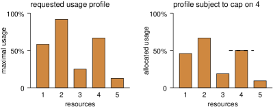
Figure 1: Illustration of a resource request profile, and how it is cut back when usage of resource 4 is limited to 50%.

But if one resource is constrained, limiting the rate of serving requests, this induces a similar reduction in the usage of all other resources (see demonstration in Fig. 1). This is essentially the “knee model” of Etsion et al. [15], where I/O activity is shown to be linearly proportional to CPU allocation up to some maximal usage level. It also corresponds to the task model of Ghodsi et al. [16] when all tasks that a user wants to execute have identical resource requirements (which is indeed the specific model they use in their proofs). Note, however, that this is indeed a limiting assumption. Specifically, it excludes usage patterns where one resource is used to compensate for lack of another resource, as happens, for example, in paging, or when using compression to reduce bandwidth.

All the above leads to the following problem definition. We want to find $x_{1},\ldots,x_{N}$, such that $0\leq x_{i}\leq 1$, where for each user $i$, $x_{i}$ is the fraction of that user’s request which will be granted. Furthermore, we require that

$$\mbox{for each resource }j:~{}x_{1}r_{1j}+\cdots+x_{N}r_{Nj}\leq 1.$$ (1)

This means that the total usage of each resource is limited by the resource capacity. Those resources for which equality holds are the bottleneck resources.

Among all the allocations $x_{1},\ldots,x_{N}$ that satisfy Eq. (1), which should qualify as “fair”? This is where we define the “no justified complaints” condition:

=1pt No Justified Complaints Condition A user cannot justify complaining about his allocation if either he gets all he asked for, or else he gets his entitlement, and giving him more would come at the expense of other users who have their own entitlements.

Using the notation above, the “no justified complaints” condition can be formally expressed as:

$$\begin{array}[]{l}\mbox{for all users }i:x_{i}=1\mbox{ or }\\ ~{}~{}~{}~{}\mbox{there exists a bottleneck resource $j^{*}$ such that }x_{i}r_{ij^{*}}\geq e_{i}.\end{array}$$ (2)

Specifically, user $i$ cannot complain if there exists some bottleneck resource $j^{*}$ where he gets at least what he is entitled to. Since $j^{*}$ is already utilized to its full capacity, giving him more, that is, increasing $x_{i}$, would necessarily come at the expense of other users, who have the right to their own entitlements. Therefore, increasing $i$’s allocation at their expense would be unfair.

Note that it may happen that a user receives less than his entitlement on other resources, including other bottleneck resources, where the entitlement would seem to indicate that a larger allocation is mandated. This is where the proportional resource usage assumption comes in. Recall that the factor $x_{i}$ is common to all resources. Thus giving a user a higher allocation on any resource implies that his allocation must grow on all resources. The original bottleneck resource $j^{*}$ thus constrains all allocations, even on other bottleneck resources or resources that are not themselves contended.

Being based on bottlenecks, it is easy to see that allocations that satisfy Eqs. (1) and (2) are Pareto optimal (but, of course, not every Pareto-optimal solution satisfies our fairness criterion). Showing that such a fair allocation exists turns out to be surprisingly nontrivial. The obvious greedy approach does not seem to work. Given a collection of requests and entitlements, suppose that we try to satisfy the users one at a time, so that, after the $k$th step, we have an allocation $(x_{1},\ldots,x_{N})$ satisfying Eq. (1) such that the first $k$ users have no complaints (that is, Eq. (2) holds for users $1,\ldots,k$). To see why doing this does not seem helpful, suppose that there are three resources and three users. User 1 requests $(\frac{1}{2},\frac{1}{2},\frac{2}{3})$ (i.e., $r_{11}=\frac{1}{2}$, $r_{12}=\frac{1}{2}$, and $r_{13}=\frac{2}{3}$) and is entitled to $0.5$ of the resources (i.e., $e_{1}=\frac{1}{2}$). User 2 requests $(\frac{1}{2},\frac{5}{8},\frac{1}{2})$ and $e_{2}=\frac{3}{8}$, and User 3 requests $(1,1,\frac{1}{3})$ with $e_{3}=\frac{1}{8}$. We start by giving user 1 everything he asks for, and users 2 and 3 nothing; that is, we consider the allocation $x=(1,0,0)$. Clearly at this point User 1 has no complaints. Next we try to satisfy User 2. If we do not cut back User 1, then we must have $x_{2}\leq\frac{2}{3}$, since resource 3 then becomes a bottleneck. But with the allocation $x=(1,\frac{2}{3},0)$ User 2 has a justified complaint: the only resource on which he gets at least his entitlement is resource 2, but resource 2 is not a bottleneck with this allocation. So User 2 feels that he is entitled to a bigger share of the resources. There are various ways to solve this problem. For example, we could consider the allocation $(\frac{3}{4},1,0)$. It is easy to check that neither User 1 nor User 2 has a justified complaint with this allocation. But now we need to add User 3 to the mix. To do so, we have to cut back either User 1 or User 2, or both. It follows from our main theorem that this can be done in a way that none of the users has a justified complaint. But the naive greedy construction does not work; at each stage, we seem to have to completely redo the previous assignment. Although a more clever greedy approach might work, we suspect not; a more global approach seems necessary. We will describe such an approach in Section 5.

4 Properties of Allocations with No Justified Complaints

In their analysis of dominant resource fairness, Ghodsi et al. [16] show that it possesses four desirable attributes, under the assumption that all tasks that a user wants to execute have identical resource requirements (in which case their model reduces to ours). We now show that our definition possesses them as well. This answers Ghodsi et al.’s question of whether there are other fair allocation schemes with these properties.

The first attribute is providing an incentive for sharing: the allocation given to each user should be better than just giving him his entitlement of each resource (actually they defined this requirement only in the case that all users are viewed as having equal entitlements, in which case this amounts to giving each user $\frac{1}{n}$th of each resource). Suppose that if user gets a fraction $e_{i}$ of each resource, he can perform a fraction $x$ of his requests, where $xr_{ij}\leq e_{i}$. In an allocation that is far in our sense, user $i$ gets to perform a fraction $y$ of his reuqests, where $yr_{ij}=e_{i}$ for some resource $j$. Thus, we must have $x\leq y$, which means that player $i$ is at least as well off participating in the scheme as he would be if he got his entitlement on each resource.

The second attribute is being strategyproof. This means that users won’t benefit from lying about their resource needs. Asking for less than the real requirements obviously just caps the user’s potential allocation at lower levels. Asking for more with the same profile (that is, same relative usage of different resources) does not have an effect, except that the user might be allocated more than he can use. While this may lead to waste, it does not provide any benefit to the user. Modifying the profile will either give the user extra capacity he can’t use on some resource, or worse, reduce the effective allocation because some unneeded resource was inflated and tricked the system into thinking it has satisfied the user’s entitlement. Thus lying cannot lead to benefits, but can in fact cause harm to a user’s allocation.

The third attribute is that the produced allocation be envy free: no user should prefer another user’s allocation. This follows from being strategy proof; otherwise a user could lie about his requirements so as to mimic those of the other user.

The fourth and final attribute is Pareto efficiency. This means that increasing the allocation to one user must come at the expense of another. As noted above, this follows from doing allocations based on bottlenecks.

We now turn to comparing our definition of fairness with dominant resource fairness. While similar in spirit, the two definitions are actually quite different in their philosophy. At a very basic level, the notion of fairness depends on perception of utility. In the context of allocating resources on computer systems, the utility is typically unknown. Consequently the notion of fairness is ill-defined.

To better understand the difference between utility and allocation, we recount an example used by Yaari and Bar-Hillel [35]. Jones and Smith are to share a certain number of grapefruit and avocados to obtain certain vitamins they need. They have different physiological abilities to extract these vitamins from the different fruit. The overwhelming majority of those polled agreed that the most fair division is one that gives them equal shares of extracted vitamins, despite being quite far from being equal shares of actual fruit. But such considerations would be impossible if you do not know their specific ability to extract vitamins, and that they actually only eat fruit for their vitamins.

When allocating resources to virtual machines or users of a cloud system, we do not know the real utility of these resources for the users. We are therefore forced to just count the amount of resources being allocated. The difference between definitions of fairness is in how this counting is done. In asset fairness, the fractions of all resources used are summed up. Thus if a user gets 20% of the CPU, 7% of the disk bandwidth, and 37% of the network bandwidth, he is considered as having received 64/300 of the total resources in the system. In order to be fair, other users should also get similar total fractions. In dominant resource fairness, only the largest fraction is considered. Thus, in the example above, the user’s dominant resource is the network, and he is considered to have received resources at a level of 37/100. To be fair, other users should receive similar levels of their respective dominant resources. In our definition of fairness, we do not focus on the dominant resource of each user, but rather take a system-wide view based on bottlenecks. Thus, if the CPU happens to be the only bottleneck, we say that this user received resources at a level of 20/100. The fact that he received more of another resource, namely the network, is immaterial, because there is no contention for the network. A user is welcome to use as much of any resource for which there is no contention as he likes.

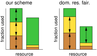
Figure 2: Example of the effect of imposing equal shares of a bottleneck resource, compared with dominant resource fairness.

Interestingly, Ghodsi et al. prove that under dominant resource fairness each user will be constrained by some resource that is a bottleneck [16]. However, their fairness criterion does not depend on this bottleneck, while ours does. The following example may help to illustrate the differences (Fig. 2). Consider a scenario with three users and two resources. The requirements of the users are $r_{1}=(1,0.2)$, $r_{2}=(1,0.2)$, and $r_{3}=(0.4,0.8)$. The entitlements are $e_{1}=e_{2}=e_{3}=\frac{1}{3}$. Obviously resource 1 is a bottleneck, so the allocations with our definition of fairness will be $a_{1}=(\frac{1}{3},\frac{2}{30})$, $a_{2}=(\frac{1}{3},\frac{2}{30})$, and $a_{3}=(\frac{1}{3},\frac{2}{3})$. This is fair on the bottleneck resource, and each user receives his entitlement. Dominant resource fairness, in contrast, leads to the following allocation: $a_{1}=(0.4,0.08)$, $a_{2}=(0.4,0.08)$, and $a_{3}=(0.2,0.4)$. User 3’s usage of resource 2 is counted, despite the fact that there is no contention for resource 2; this leads to a reduced allocation of resource 1. There seems to be no criteria by which to say that one allocation is fairer than the other. It may well be that user 3 derives much benefit from using resource 2, and therefore cutting him back on resource 1 is perfectly justified. But given that we do not know that this is the case, we suggest that it is safer to focus on the bottleneck resources.

In fact, Ghodsi et al. do mention bottleneck fairness in their description of dominant resource fairness, but only as a secondary criterion. They define bottleneck fairness only when all users have the same dominant resource, essentially reducing the scope to the single bottleneck case. Our work is the first to extend this with a meaningful definition of fairness for multiple bottlenecks, and when the dominant resources are different.

We now turn to a few more observations of the relationship between our definition and dominant resource fairness. First, we observe that if all users have the same dominant resource, dominant resource fairness and our definition are equivalent. This follows since the common dominant resource is the only bottleneck.

Another interesting question is one of utilization. In the example given above, our definition of fairness led to higher overall utilization than dominant resource fairness. It this guaranteed to always be the case? The answer is no, as the following counter-example demonstrates. Assume two users and four resources, with requirement vectors of $r_{1}=(\frac{1}{2},0,0,1)$ and $r_{2}=(1,1,1,0)$ and equal entitlements $e_{1}=e_{2}=\frac{1}{2}$. With our no justified complaints definition, the first and last resources are the bottlenecks, and the allocations are $a_{1}=(\frac{1}{2},0,0,1)$ and $a_{2}=(\frac{1}{2},\frac{1}{2},\frac{1}{2},0)$. If there were many more “middle” resources, the average utilization would tend to $\frac{1}{2}$. With the dominant resource fairness scheme, the allocations are $a_{1}=(\frac{1}{3},0,0,\frac{2}{3})$ and $a_{2}=(\frac{2}{3},\frac{2}{3},\frac{2}{3},0)$. In this case, the average utilization tends to $\frac{2}{3}$.

Another important difference between the two definitions is that dominant resource fairness allocations can be found using an incremental algorithm [16]. Finding allocations based on the no justified complaints idea is harder, because we do not know in advance which resources will be the bottlenecks. Nevertheless, the proof presented in the next section shows that such an allocation always exists. Moreover, the trajectory argument used is actually somewhat similar to how allocations are constructed for dominant resource fairness.

5 Existence of a Fair Allocation

In this section, we prove that an allocation satisfying (1) and (2) always exists. Note, however, that there is an additional requirement that $x_{i}\leq 1$, and that (2) makes a distinction between the case $x_{i}<1$ (need to exceed entitlement on some bottleneck resource) and the case $x_{i}=1$ (get all you want). We can treat these two cases uniformly by defining $N$ dummy resources that are each requested by only one user. Using $m^{\prime}$ to denote the number of real resources, we define the requirements on the dummy resources to be $r_{i,m^{\prime}+i}=1$ for $i=1,\ldots,N$, and $r_{i,j}=0$ for $i=1,\ldots,N$, $j=m^{\prime}+1,\ldots,m^{\prime}+N$, and $j\neq m^{\prime}+i$. These dummy resources can only become a “bottleneck” if their corresponding $x_{i}=1$, meaning that the user gets all he requested. In the following, $m$ will denote the full set of resources including the dummy ones.

With this addition, we want to prove the following:

Theorem 1.

Given

• entitlements $e_{1},\ldots,e_{N}$ such that $e_{1}+\cdots+e_{N}=1$ and $e_{i}\geq 0$ for $i=1,\ldots,N$, and

• resource requirements $r_{ij}$, $i=1,\ldots,N$, $j=1,\ldots,m$ such that $r_{1j}+\cdots+r_{Nj}\geq 1$ for $j=1,\ldots,m$ and $0\leq r_{ij}\leq 1$ for $i=1,\ldots,N$ and $j=1,\ldots,m$,

there exists an allocation $x_{1},\ldots,x_{N}$, where $0\leq x_{i}\leq 1$ for $i=1,\ldots,N$, that satisfies the two conditions

1. for all resources $j$, $j=1,\ldots,m$,   $x_{1}r_{1j}+\cdots+x_{N}r_{Nj}\leq 1$;

2. for all users $i$, $i=1,\ldots,N$, there exists a resource $j^{*}$ such that $x_{i}r_{ij^{*}}\geq e_{i}$ and $x_{1}r_{1j^{*}}+\cdots+x_{N}r_{Nj^{*}}=1$.

As the mathematical derivation is somewhat involved, we first provide an argument for the special case $N=2$ (two users); this enables us to draw the constructions used in 2D. The full proof for all values of $N$ is given in Section 5.4.

5.1 Simplifying Assumptions

Before proving the theorem, we make three simplifying assumptions, all without loss of generality. First, as reflected in the definition of the resource requirements, we assume that, for each resource $j$, $r_{1,j}+\cdots+r_{Nj}\geq 1$. If there is any additional resource $j^{\diamond}$ for which this inequality does not hold, we can ignore resource $j^{\diamond}$, and solve the problem for the remaining resources. Whatever solution we come up with will also be a solution when we add $j^{\diamond}$ back to the picture, because its usage will be at most $r_{1,j^{\diamond}}+\cdots+r_{Nj^{\diamond}}<1$.

Second, we assume that, for each user $i$, there is at least one resource $j$ such that $r_{ij}\geq e_{i}$. (This pertains to only real resources, not the dummy resources.) If this is not the case, we give user $i$ everything he asked for, remove his requests, renormalize the entitlements of the remaining users so that they still sum to 1, renormalize the remaining capacity of the different resources so that it is still 1, and renormalize the remaining requests by the same factors. For example, suppose that users 1, 2, and 3 are entitled to 0.5, 0.2, and 0.3 of capacity, respectively. If User 1 never asks for more than 0.5 of any resource, then we give him what he asks for, and remove his requests from the picture. Note that this means that, for each resource $r$, the fraction of $r$ available is at least as much as the entitlement of each user. We then multiply User 2 and User 3’s entitlements by 2 ($=1/(1-0.5)$), so that their entitlements still sum to 1. After this normalization, they are entitled to 0.4 and 0.6 of what remains after we have granted User 1’s request. Moreover, if User 1 requested, say, 0.4 of Resource 1, so that 60% of Resource 1 is still available, we multiply each of the remaining user’s requests by $\frac{5}{3}$ ($=1/0.6$). Again, if we solve the resulting problem, we will have solved our original problem. This follows in general since, if User 1 is the one eliminated, the entitlements of the remaining users effectively grew by a factor of $1/(1-e_{1})$, while the requests and capacity of resource $j$ grew by $1/(1-r_{1j})$. Since $r_{1j}<e_{1}$ the entitlements grew by a larger factor, and fulfilling them will also satisfy the original entitlements.

Finally, we assume that there are no dominated inequalities, where an inequality $x_{1}r_{1j}+\cdots+x_{N}r_{Nj}\leq 1$ is dominated if any solution $(x_{1},\ldots,x_{N})$ to the remaining inequalities is also a solution to this inequality. Dominated inequalities can be efficiently found by standard linear programming methods. We can clearly remove dominated inequalities to get a system with no dominated inequalities. Depending on the order of removal, we may end up with different systems. However, a solution to any of the undominated systems is also a solution to the original system.

We now prove that we can find a solution $x_{1}\ldots x_{N}$ satisfying the requirements of Theorem 1 under these simplifying assumptions. We stress that this is without loss of generality; as shown above, if we can find a solution under the simplifying assumptions, we can also find one without these assumptions.

5.2 Proof Structure

We first establish some notation. By (1), the set of legal allocations is a subset $\mathcal{D}$ of $\mathbb{R}^{N}$, where

$$\begin{array}[]{l@{\,}l}\mathcal{D}=\{&(x_{1},\dots,x_{N}):\,\,0\leq x_{i}\leq 1,\,\,\forall i\quad\text{ and }\\ &x_{1}r_{1j}+\cdots+x_{N}r_{Nj}\leq 1,\,\,\forall j\>\}.\\ \end{array}$$

For $N=2$, this is a polygon in the first quadrant, as illustrated in Fig. 3. In the figure, two users contend for three resources ($m=3$). The request vectors are $r_{1}=(\frac{1}{4},\frac{2}{3},1)$ and $r_{2}=(1,\frac{2}{3},0)$. This leads to the bounds shown; for example, the point $(\frac{2}{3},\frac{11}{12})$ is impossible because it would imply using $\frac{2}{3}\cdot\frac{1}{4}+\frac{11}{12}\cdot 1=\frac{13}{12}$ of resource 1, i.e. more than its capacity. In the general case, this region is a simplex in the positive orthant (that is, the convex hull of $N$ affinely independent points, all in $(\mathbb{R}^{+})^{N}$).

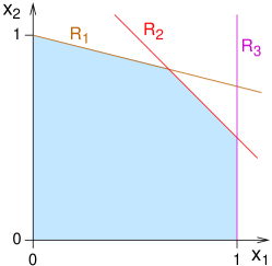
Figure 3: Depiction of bounds on $x_{i}$ values due to capacity constraints of resources, for $N=2$ and $m=3$.

For every vector $\boldsymbol{x}=(x_{1},\dots,x_{N})$ in $\mathcal{D}$, the set of bottleneck resources is

$$J(\boldsymbol{x})=\{j:\,\,1\leq j\leq m,\quad x_{1}r_{1j}+\cdots+x_{N}r_{Nj}=1\}.$$

$J(\boldsymbol{x})$ is empty for all $\boldsymbol{x}$ in the interior of the domain $\mathcal{D}$, implying that our solution will lie on the boundary of $\mathcal{D}$. Using this notation to re-write requirement (2), our goal is to prove that there exists an allocation $\boldsymbol{x}=(x_{1},\dots,x_{N})$, such that

$$\begin{array}[]{l}\mbox{for every~{}}~{}i=1,\dots,N{}\\ ~{}~{}~{}~{}~{}\mbox{~{}there exists a~{}}j\in J(\boldsymbol{x})\mbox{~{}such that~{}}x_{i}r_{ij}\geq e_{i}.\end{array}$$ (3)

The difficulty in finding $\boldsymbol{x}$ stems exactly from this condition. In fact, if we knew what the bottleneck resources would be, the problem could be solved efficiently using well-known machinery. Specifically, fix an arbitrary subset $I\subseteq\{1,\ldots,m\}$, and consider the following decision problem: Is there an $\boldsymbol{x}\in\mathcal{D}$ for which $J(\boldsymbol{x})=I$ such that condition (3) holds? It can easily be verified that this is asking whether a finite set of linear equations and linear inequalities is consistent. This task is subsumed by the Linear Programming problem, and can thus be solved in polynomial time.

How can we overcome the difficulty involved in satisfying condition (3) without knowing in advance what the set $J(\boldsymbol{x})$ is? We take a somewhat unconventional approach to this problem. The set $\mathcal{D}$ is a polytope, that is, a bounded convex subset of $\mathbb{R}^{N}$ that is defined by a finite list of linear inequalities. We want to approximate $\mathcal{D}$ by a subset $\cal{Q}\subseteq\mathcal{D}$ that is convex and has a smooth boundary. Intuitively, $\cal{Q}$ “rounds off” the corners of $\mathcal{D}$ (see below for further discussion). Such a set $\mathcal{Q}$ is defined by infinitely many linear inequalities: For every hyperplane $H$ that is tangent to $\mathcal{Q}$ we write a linear inequality that states that $\boldsymbol{x}$ must reside “below” $H$. It would seem that this only complicates matters, replacing the finitely defined $\mathcal{D}$ by $\mathcal{Q}$. However, the problematic condition (3) takes on a much nicer form when applied to $\mathcal{Q}$, and becomes a very simple relation involving the contact point of $H$ and $\mathcal{Q}$, the normal to $H$, and the vector $e$ (see Equation (7) below). Moreover, using standard tools from the theory of ordinary differential equations, we can find a point on the boundary of $\mathcal{Q}$ where this relation holds.

To find the solution, we do not consider a single smooth $\mathcal{Q}$, but rather a whole parametric family $\mathcal{Q}_{t}$. This family has the properties that (a) the sets $\mathcal{Q}_{t}$ grow as the parameter $t$ increases; (b) they are all contained in $\mathcal{D}$; and (c) as $t\rightarrow\infty$ the sets $\mathcal{Q}_{t}$ converge to $\mathcal{D}$. For every $t>0$, we find a point $\boldsymbol{x}^{(t)}$ on the boundary of $\mathcal{Q}_{t}$ such that $\boldsymbol{x}^{(t)}$ satisfies the analogue of condition (3). As $t\rightarrow\infty$ the points $\boldsymbol{x}^{(t)}$ tend to the boundary of $\mathcal{D}$. We argue that there always exists a convergent subsequence of the points $\boldsymbol{x}^{(t)}$, and show that the limit point of this subsequence solves our original problem. In the language of the description below, $\mathcal{Q}_{t}$ is defined as the set of those $\boldsymbol{x}\in\mathcal{D}$ for which $f(\boldsymbol{x})\leq t$.

The procedure above hinges on our ability to define the appropriate points $\boldsymbol{x}^{(t)}$ that satisfy the required condition. This is based on considering the tangent to the surface of $\mathcal{Q}_{t}$. Note that the only essential difference between $\mathcal{D}$ and $\mathcal{Q}$ is that the latter is defined by an infinite family of defining linear inequalities, namely, one for each hyperplane $H$ that is tangent to $\mathcal{Q}$. Keeping this perspective in mind, let us apply the original problem definition to a point $\boldsymbol{x}\in\mathcal{Q}$. If $\boldsymbol{x}$ lies in the interior of $\mathcal{Q}$, then none of $\mathcal{Q}$’s defining inequalities holds with equality. Thus, as before, $J(\boldsymbol{x})$ is empty for any $\boldsymbol{x}$ in the interior of the domain $\mathcal{Q}$. We therefore consider $\boldsymbol{x}$ that lies on the boundary of $\mathcal{Q}$. In this case the set $J(\boldsymbol{x})$ is a singleton, the only member of which is the inequality corresponding to the hyperplane $H$ that is tangent to $\mathcal{Q}$ and touches it at the point $\boldsymbol{x}$. The equation of the tangent hyperplane $H$ can be written as $\sum\nu_{i}x_{i}=1$, where the vector $(\nu_{1},\ldots,\nu_{n})$ is normal to $H$. Now condition (3) becomes

$$\forall i~{}~{}~{}\nu_{i}x_{i}\geq e_{i}.$$ (4)

When we sum over all $i$ this becomes $\sum\nu_{i}x_{i}\geq\sum e_{i}=1$. But $\boldsymbol{x}$ lies on $H$, so that $\sum\nu_{i}x_{i}=1$. It follows that all inequalities in Eq. (4) hold with equality. But we also have, from the definition of the bottlenecks, that $\sum r_{ij}x_{i}=1$. Thus, the normal is simply defined by the requirements vectors. Moreover, we can use this as a condition on the gradients of the surfaces of $\mathcal{Q}_{t}$ for successive $t$’s, and follow a trajectory that leads to a solution on the boundary of $\mathcal{D}$. This is then the desired constructive proof: it both shows that a solution exists, and provides a mechanism for finding it.

5.3 The Case $N=2$

In this section, we give a complete proof of Theorem 1 for the case $N=2$ that is simpler than our general proof, and is perhaps more intuitive. This includes an explanation of the relationship between the normals to the surfaces and the requirements vectors. The argument for arbitrary $N$ is given in the next subsection.

In the case $N=2$, as noted above, the constraint (1) defines a region in the first quadrant whose boundary is a piecewise linear curve that satisfies the constraints in (1) with $\leq$ replaced by $=$. Note that the slopes of the lines that define the boundary are negative, and as $k$ increases from 0 to 1, the slopes of the lines that intersect the vertical line $x=k$ get more and more negative. This follows from the fact that the interior is convex.

Let $g$ be the piecewise linear curve that defines the boundary. We can approximate $g$ arbitrarily closely from below by a concave twice-differentiable function $f$. (The function $g$ is the boundary of the region called $\mathcal{D}$ in the previous section; the function $f$ is the boundary of the region $\mathcal{Q}$.) The concavity of the curve $f$ just means that $f^{\prime\prime}<0$. As we said earlier, $f$ “rounds off” the corners of $g$, as shown in Fig. 4.

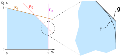
Figure 4: Rounding off the boundary of $\mathcal{D}$.

As we said in the previous section, we want to find a point $(x_{1}^{*},x_{2}^{*})$ on the curve $f$ such that if $\nu_{1}x_{1}+\nu_{2}x_{2}=1$ is the tangent to the curve at $(x_{1}^{*},x_{2}^{*})$, then $\nu_{1}x_{1}^{*}=e_{1}$ and $\nu_{2}x_{2}^{*}=e_{2}$. We show below how to find such a point. We now argue that finding such a point for each $f$ approximating $g$ suffices to prove the theorem in the case that $N=2$. First suppose that $(x_{1}^{*},x_{2}^{*})$ is actually a point on one of the lines that define $g$ (as opposed to a point on $f$ that arises from rounding off a corner of the curve $g$). Suppose that the line is defined by resource $j$, so that it has the form $r_{1j}x_{1}+r_{2j}x_{2}=1$. Obviously the tangent to $f$ at the point $(x_{1}^{*},x_{2}^{*})$ on the line is just the line itself, so we have $\nu_{1}=r_{1j}$ and $\nu_{2}=r_{2j}$. Thus, we will have found $x_{1}^{*}$ and $x_{2}^{*}$ such that $r_{1j}x_{1}^{*}=e_{1}$ and $r_{2j}x_{2}^{*}=e_{2}$, which means that (2) holds (and moreover, the same resource provides justification for both users).

Next, suppose that $(x_{1}^{*},x_{2}^{*})$ is not on one of the original lines, but we can find such a point for all functions $f$ approximating $g$. Straightforward continuity arguments show that small changes to $f$ result in small changes to the point, so that as $f$ gets closer to $g$, we get a sequence of points that approach a point on $g$. Thus the limit is a point on $g$. We actually get even more. What we really have for each function $f$ that approximates $g$ is two pairs $(x_{1}^{*},x_{2}^{*})$ and $(\nu_{1},\nu_{2})$, where $(x_{1}^{*},x_{2}^{*})$ is a point on $f$, $\nu_{1}x_{1}+\nu_{2}x_{2}=1$ is the tangent to $f$ at $(x_{1}^{*},x_{2}^{*})$, $\nu_{1}x_{1}^{*}=e_{1}$, and $\nu_{2}x_{2}^{*}=e_{2}$. As $f$ approaches $g$, we will get a sequence of such pairs of points. Let $(x^{g}_{1},x^{g}_{2})$ and $(\nu_{1}^{g},\nu_{2}^{g})$ be the limit of this sequence of pairs of pairs. It is clearly the case that $(x^{g}_{1},x^{g}_{2})$ is a point on $g$, $\nu_{1}^{g}x_{1}^{g}=e_{1}$, $\nu_{2}^{g}x_{2}^{g}=e_{2}$, and $\nu_{1}^{g}x_{1}+\nu_{2}^{g}x_{2}=1$. Now if $(x^{g}_{1},x^{g}_{2})$ is in the interior of one of the lines that make up the boundary of the region — let’s assume it is the line associated with resource $j$ — then, as the argument above suggests, $\nu_{1}^{g}=r_{1j}$ and $\nu_{2}^{g}=r_{2j}$. Thus, resource $j$ is a bottleneck, and provides a justification for both users.

Now suppose that $(x^{g}_{1},x^{g}_{2})$ is at the intersection of two lines, say, representing resources $j$ and $j^{\prime}$. Thus, $x^{g}_{1}r_{1j}+x^{g}_{2}r_{2j}=1$ and $x^{g}_{1}r_{1j^{\prime}}+x^{g}_{2}r_{2j^{\prime}}=1$, so both resources are bottlenecks at $(x^{g}_{1},x^{g}_{2})$. Moreover, we still have $\nu_{1}^{g}x_{1}^{g}=e_{1}$ and $\nu_{2}^{g}x_{2}^{g}=e_{2}$. Finally, it is clear that $\nu_{i}^{g}$ must be a convex combination of $r_{ij}$ and $r_{ij^{\prime}}$, for $i\in\{1,2\}$, since, for each approximation $f$ to $g$, the tangent in the region that we have “rounded off” is a convex combination of the tangents of the lines that make up $g$ that are being approximated. It follows that each user $i\in\{1,2\}$ gets at least his entitlement on one of resources $j$ or $j^{\prime}$; that is, either $r_{ij}x_{i}^{g}\geq e_{i}$ or $r_{ij^{\prime}}x_{i}^{g}\geq e_{i}$. For if $r_{ij}x_{i}^{g}<e_{i}$ and $r_{ij^{\prime}}x_{i}^{g}<e_{i}$, then $\nu_{i}^{g}x_{i}^{g}<e_{i}$, and we have a contradiction.

The fact that we can find such a point $(x_{1}^{*},x_{2}^{*})$ on each $f$ follows from another easy continuity argument. Consider the points on the function $f$ in the first quadrant. Suppose that $f$ starts at the $Y$-axis at some point $(0,y^{\prime})$ and ends at the $X$-axis at some point $(x^{\prime},0)$. Let the equation of the tangent of $f$ at the point $\boldsymbol{x}^{\diamond}=(x_{1}^{\diamond},x_{2}^{\diamond})$ be $\nu^{\boldsymbol{x}^{\diamond}}\cdot\boldsymbol{x}=1$. Consider the term $q(\boldsymbol{x}^{\diamond})=(\nu^{\boldsymbol{x}^{\diamond}}_{1}x_{1}^{\diamond})/(\nu^{\boldsymbol{x}^{\diamond}}_{2}x_{2}^{\diamond})=-f^{\prime}(x_{1}^{\diamond})x_{1}^{\diamond}/x_{2}^{\diamond}$ as $\boldsymbol{x}^{\diamond}$ goes from $(0,y^{\prime})$ to $(x^{\prime},0)$. As $\boldsymbol{x}^{\diamond}$ approaches $(0,y^{\prime})$ from the right, $q(\boldsymbol{x}^{\diamond})$ approaches 0; as $\boldsymbol{x}^{\diamond}$ approaches $(x^{\prime},0)$ from the left, $q(\boldsymbol{x}^{\diamond})$ approaches $\infty$. Since $f^{\prime}$ is continuous, $q$ varies continuously in the first quadrant between $0$ and $\infty$. Thus, at some point it must have value $e_{1}/e_{2}$. If $q(\boldsymbol{x}^{*})=e_{1}/e_{2}$, then we must have $\nu^{\boldsymbol{x}^{*}}_{1}x_{1}^{*}/\nu^{\boldsymbol{x}^{*}}_{2}x_{2}^{*}=e_{1}/e_{2}$. Since we also have $\nu^{\boldsymbol{x}^{*}}_{1}x_{1}^{*}+\nu^{\boldsymbol{x}^{*}}_{2}x_{2}^{*}=1$ and $e_{1}+e_{2}=1$, it easily follows that we must have $\nu^{\boldsymbol{x}^{*}}_{1}x_{1}^{*}=e_{1}$ and $\nu^{\boldsymbol{x}^{*}}_{2}x_{2}^{*}=e_{2}$, as desired. This completes the proof in the case that $N=2$.

We can actually say more in the case that $N=2$. Since $f$ is concave, $f^{\prime}$ is decreasing, so $-f^{\prime}$ is increasing. It easily follows that $q$ is an increasing function. Thus, there is a unique point $(x_{1}^{*},x_{2}^{*})$ with the desired properties. It easily follows that, in the case of two users, the solution to (1) and (2) is unique. Uniqueness has an important consequence. In the problem definition, the bottleneck resources in (1) are not known in advance. In particular, it might seem that different solutions may lead to different resources becoming bottlenecks. Uniqueness guarantees that this is not the case, and that the set of resources that will become bottlenecks is uniquely defined by the problem parameters (that is, the entitlements and request profiles). We remark that the uniqueness claim does not hold in general for $N>2$; see Section 5.5.

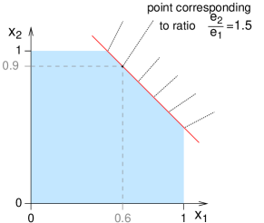
Figure 5: Simple example of a point $(x_{1}^{*},x_{2}^{*})$. Different points correspond to different ratios $\frac{e_{2}}{e_{1}}$, as indicated by the slopes of the line segments.

The example in Fig. 5 may help in gaining an intuition for the derivation above. Consider a single limiting resource, where both users request $r_{1}=r_{2}=\frac{2}{3}$ of its capacity. The boundary line representing the capacity limit of the resource has the equation $\frac{2}{3}x_{1}+\frac{2}{3}x_{2}=1$. Different points along this line correspond to different ratios of the users’ entitlements. For example, if they have entitlements of $0.4$ and $0.6$, the point $(0.6,0.9)$ satisfies the equations $\frac{2}{3}\cdot 0.6=0.4$ and $\frac{2}{3}\cdot 0.9=0.6$, and indeed using these values for $x_{1}$ and $x_{2}$ leads to sharing the resource in the desired proportions. If the ratio of entitlements is such that $\frac{e_{2}}{e_{1}}>2$, then user 2 is not requesting his full entitlement, and is eliminated from consideration. He is given his full request, and user 1 gets the rest, which is more than his entitlement (so they are both satisfied). This is in fact an example of a solution based on a dummy resource. The opposite happens if $\frac{e_{2}}{e_{1}}<\frac{1}{2}$.

5.4 Proof of Theorem 1

We now prove Theorem 1 for arbitrary $N$.

Construction 1.

To every allocation $\boldsymbol{x}$ in the interior of the domain $\mathcal{D}$, we assign a value

$$f(\boldsymbol{x})=-\sum_{j=1}^{m}\log\left(1-\sum_{k=1}^{N}x_{k}r_{kj}\right).$$ (5)

Remark 1.

The function $f$ is positive in the interior of $\mathcal{D}$, diverging to infinity as $\boldsymbol{x}$ tends to the boundary of $\mathcal{D}$.

Remark 2.

Clearly, there are other choices of $f$ that satisfy these desired properties. This choice seems like the simplest one for our purposes.

Definition 1.

To every number $t>0$, there corresponds a level set of $f$, namely,

$$\Gamma_{t}=\{\boldsymbol{x}\in\mathcal{D}:\,\,f(\boldsymbol{x})=t\},$$

Remark 3.

This is an $(N-1)$-dimensional hypersurface. (Fig. 6 illustrates this for $N=2$.)

Definition 2.

To every point $\boldsymbol{x}\in\mathcal{D}$, there corresponds a unique unit vector $\boldsymbol{\nu}(\boldsymbol{x})=(\nu_{1}(\boldsymbol{x}),\dots,\nu_{N}(\boldsymbol{x}))$, normal to the level set of $f$ at $\boldsymbol{x}$.

The unit normal $\boldsymbol{\nu}(\boldsymbol{x})$ is proportional to the gradient of $f$ at $\boldsymbol{x}$, implying that

$$\nu_{i}(\boldsymbol{x})=\tilde{c}\,\frac{\partial f}{\partial x_{i}}(\boldsymbol{x})=\tilde{c}\sum_{j=1}^{m}\frac{r_{ij}}{1-\sum_{k=1}^{N}x_{k}r_{kj}},\quad\forall i=1,\dots,N,$$ (6)

where the normalization constant $\tilde{c}$ is chosen so as to guarantee that $\boldsymbol{\nu}$ is a unit vector, that is, $\nu_{1}^{2}+\dots+\nu_{N}^{2}=1$.

\psfrag{infty}{$\infty$}\includegraphics[width=130.08731pt]{waves.eps}

Figure 6: Illustration of level-sets of $f$ from $t=0$ to $t=\infty$.

Construction 2.

We now construct a vector-valued function

$$\boldsymbol{x}(t)=(x_{1}(t),\dots,x_{N}(t)),\qquad t\geq 0,$$

satisfying the following properties:

1. $\boldsymbol{x}(t)$ lies on the level set $\Gamma_{t}$ for all $t\geq 0$ (and, in particular, remains in $\mathcal{D}$).

2. For all $t>0$, there exists a $t$-dependent normalization factor $c(t)$, such that for every $i=1,\dots,N$,

   $$x_{i}(t)\,\nu_{i}(\boldsymbol{x}(t))=\tilde{c}\,c(t)e_{i}.$$ (7)

Remark 4.

Note that since $f(\boldsymbol{x}(0))=0$ it follows that $\boldsymbol{x}(0)=0$, that is, the vector-valued function $\boldsymbol{x}(t)$ “starts” at the origin.

Remark 5.

substituting (6) into (7) and summing over the index $i$ determines $\tilde{c}\,c(t)$. After simple algebraic manipulations, summing the expressions (7) over $i$ gives us

$$\sum_{j=1}^{m}\frac{x_{i}(t)r_{ij}-(\sum_{k=1}^{N}x_{k}(t)r_{kj})e_{i}}{1-\sum_{k=1}^{N}x_{k}(t)r_{kj}}=0,\;\forall i=1,\dots,N,\,\,\forall t>0.$$ (8)

Intuitively, $\boldsymbol{x}(t)$ is a “trajectory” that takes us from the origin $\boldsymbol{x}=0$ to a point on the boundary of $\mathcal{D}$ as $t$ grows from $0$ to $\infty$.

The formal proof now follows from the following sequence of three lemmas, proved below. First, we show that a trajectory with the required properties exists (Lemma 4). Given such a trajectory, we show that a subsequence of this trajectory converges to a point on the boundary of $\mathcal{D}$ (Lemma 2). Finally, this accumulation point is shown to be a solution to our allocation problem (Lemma 3).

It is convenient to delay the question of whether there indeed exists a trajectory $\boldsymbol{x}(t)$ satisfying the required properties, and consider convergence first.

Lemma 2.

Let $0<t_{1}<t_{2}<\cdots$ be a sequence tending to infinity. Let $x(t)$ be a vector-valued function as defined in Construction 2. Then, the sequence $x(t_{i})$ has a subsequence that converges to an allocation $\boldsymbol{x}^{*}$ on the boundary of $\mathcal{D}$.

Proof.

Consider what happens as $t\to\infty$. Since $\boldsymbol{x}(t)\in\Gamma_{t}$, it follows that $\boldsymbol{x}(t)$ approaches the boundary of $\mathcal{D}$. However, the function $\boldsymbol{x}(t)$ may not tend to a limit as $t\to\infty$. Nevertheless, since $\mathcal{D}$ is a compact domain, $\boldsymbol{x}(t)$ has a convergent subsequence. That is, there exists an allocation $\boldsymbol{x}^{*}=(x_{1}^{*},\dots,x_{N}^{*})$ on the boundary of $\mathcal{D}$ and a subsequence $t_{n_{1}}<t_{n_{2}}<\dots$ such that

$$\lim_{k\to\infty}\boldsymbol{x}(t_{n_{k}})=\boldsymbol{x}^{*}.$$

∎

The next lemma shows that this accumulation point is a solution to the fair allocation problem.

Lemma 3.

An allocation $\boldsymbol{x}^{*}$ as resulting from Lemma 2 is a fair allocation according to our definition.

Proof.

Since $\boldsymbol{x}^{*}$ is on the boundary of $\mathcal{D}$, it has a non-empty set $J(\boldsymbol{x}^{*})$ of bottleneck resources such that

$$x^{*}_{1}r_{1j}+\dots+x_{N}^{*}r_{Nj}=1\qquad\forall j\in J(\boldsymbol{x}^{*})\neq\emptyset.$$

We then rewrite (8) by splitting the resources $j$ into bottleneck resources and non-bottleneck resources, and setting $t=t_{n}$:

$$\begin{array}[]{l}\displaystyle\sum_{j\not\in J(\boldsymbol{x}^{*})}\frac{x_{i}(t_{n})r_{ij}-(\sum_{k=1}^{N}x_{k}(t_{n})r_{kj})e_{i}}{1-\sum_{k=1}^{N}x_{k}(t_{n})r_{kj}}\>+\\[17.07164pt] \displaystyle\sum_{j\in J(\boldsymbol{x}^{*})}\frac{x_{i}(t_{n})r_{ij}-(\sum_{k=1}^{N}x_{k}(t_{n})r_{kj})e_{i}}{1-\sum_{k=1}^{N}x_{k}(t_{n})r_{kj}}=0.\end{array}$$ (9)

The two summations behave very differently as $n\to\infty$. For a non-bottleneck resource $j$, $\sum_{k=1}^{N}x_{k}^{*}r_{kj}<1$, so the summation over the non-bottleneck resources tends to a limit obtained by letting $\boldsymbol{x}(t_{n})\to\boldsymbol{x}^{*}$ term-by-term:

$$\begin{array}[]{l}\displaystyle\lim_{n\to\infty}\sum_{j\not\in J(\boldsymbol{x}^{*})}\frac{x_{i}(t_{n})r_{ij}-(\sum_{k=1}^{N}x_{k}(t_{n})r_{kj})e_{i}}{1-\sum_{k=1}^{N}x_{k}(t_{n})r_{kj}}\\[17.07164pt] \displaystyle=\sum_{j\not\in J(\boldsymbol{x}^{*})}\frac{x_{i}^{*}r_{ij}-(\sum_{k=1}^{N}x_{k}^{*}r_{kj})e_{i}}{1-\sum_{k=1}^{N}x_{k}^{*}r_{kj}}.\end{array}$$ (10)

For a bottleneck resource $j$, the denominator $1-\sum_{k=1}^{N}x_{k}r_{kj}$ tends to zero as $x\to x^{*}$, so the limit exists only if the numerator vanishes as well. But if it were the case that, for a given user $i$,

$$x^{*}_{i}r_{ij}<e_{i}\qquad\mbox{ for all }j\in J(\boldsymbol{x}^{*}),$$

then

$$\lim_{n\to\infty}\sum_{j\in J(\boldsymbol{x}^{*})}\frac{x_{i}(t_{n})r_{ij}-(\sum_{k=1}^{N}x_{k}(t_{n})r_{kj})e_{i}}{1-\sum_{k=1}^{N}x_{k}(t_{n})r_{kj}}=-\infty.$$

This is a contradiction to the fact that, by (9), the limit should be the negative of the right-hand side of (10). Hence we conclude that $\boldsymbol{x}^{*}$ has the property that for all users $i$, there exists a bottleneck resource $j$ such that $x^{*}_{i}r_{ij}\geq e_{i}$. Thus, $\boldsymbol{x}^{*}$ is a fair allocation. ∎

It remains to show that the trajectory $\boldsymbol{x}(t)$ is indeed well-defined for all system parameters $e_{i}$ and $r_{ij}$. This is handled by the following lemma.

Lemma 4.

There exists a function $\boldsymbol{x}(t)$ with the properties specified in Construction 2.

Proof.

To prove this we show that we can find points satisfying property 1 that also satisfy property 2. Since $\boldsymbol{x}(t)\in\Gamma_{t}$, we have $f(x(t))=t$, that is,

$$-\sum_{j=1}^{m}\log\left(1-\sum_{k=1}^{N}x_{k}(t)r_{kj}\right)=t.$$ (11)

By (7),

$$\sum_{j=1}^{m}\frac{x_{i}(t)r_{ij}}{1-\sum_{k=1}^{N}x_{k}(t)r_{kj}}=c(t)e_{i},\qquad\forall i=1,\dots,N.$$ (12)

Differentiating both equations with respect to $t$, we obtain a linear system of equations for the derivative $d\boldsymbol{x}/dt$. Differentiating (11), we get

$$\frac{\sum_{k=1}^{N}\frac{dx_{k}}{dt}r_{kj}}{1-\sum_{k=1}^{N}x_{k}(t)r_{kj}}=1.$$

Differentiating (12), we get

$$\sum_{j=1}^{m}\frac{\frac{dx_{i}}{dt}r_{ij}}{1-\sum_{k=1}^{N}x_{k}r_{kj}}+\sum_{j=1}^{m}\frac{x_{i}r_{ij}\sum_{k=1}^{N}\frac{dx_{k}}{dt}r_{kj}}{(1-\sum_{k=1}^{N}x_{k}r_{kj})^{2}}=\frac{dc}{dt}e_{i}.$$ (13)

Observe that, without loss of generality, we can set $dc/dt=1$, compute the resulting vector of derivatives $d\boldsymbol{x}/dt$, and then multiply it by a constant for the normalization condition to hold. Thus, it remains only to show that (13) has a unique solution when $dc/dt=1$. To do so, we define an $\boldsymbol{x}$-dependent matrix with entries

$$b_{ij}=\frac{r_{ij}}{1-\sum_{k=1}^{N}x_{k}r_{kj}},\qquad i=1,\dots,N,\qquad j=1,\dots,m\;.$$

These entries are non-negative for $\boldsymbol{x}\in\mathcal{D}$. We now rewrite (13) in a more compact form,

$$\sum_{k=1}^{m}\frac{dx_{k}}{dt}\left(\sum_{j=1}^{m}b_{ij}\delta_{ik}+\sum_{j=1}^{N}x_{i}b_{ij}b_{kj}\right)=e_{i}.$$

The term inside the brackets is the $(k,i)$ entry of a symmetric positive-definite $N\times N$ matrix, which immediately implies that there exists a unique solution $d\boldsymbol{x}/dt$. Moreover, since the dependence of $d\boldsymbol{x}/dt$ on $\boldsymbol{x}$ is continuous, the existence and uniqueness of $\boldsymbol{x}(t)$ follows from the Fundamental Theorem of Ordinary Differential Equations [9]. (More precisely, the fundamental theorem of ODEs guarantees only the existence and uniqueness of a solution for some small $t$; global existence follows from the boundedness of the domain $\mathcal{D}$.) ∎

This completes the proof of Theorem 1.

We note that our proof that a fair allocation exists is almost constructive. The trajectories $\boldsymbol{x}(t)$ can easily be computed numerically using standard ODE integrators (for example, Matlab’s ode45 function). If $\boldsymbol{x}(t)$ is found to tend to a limit for large $t$, then this limit is a fair allocation. The only reservation is that numerical integration only provides approximate solutions (however, with a controllable error), and can only be carried out over a finite $t$ interval.

5.5 Uniqueness of the Solution

As we mentioned in Section 5.3, unlike the case $N=2$, in the general case the solution is not unique. This is easily seen from the following counterexample. Assume $N=3$ and $m=2$, with $r_{1}=(1,1)$, $r_{2}=(0,1)$, $r_{3}=(1,0)$, and $e=(0.5,0.3,0.2)$. This has the the family of solutions $x=(z,1-z,1-z)$ for $z$ that satisfies $0.5\leq z\leq 0.7$, where in all these solutions both resources are bottlenecks. Note that this does not contradict the fact that our solution method finds a unique trajectory. This trajectory corresponds to the choice of the function $f$ in (5). Other choices, e.g. by adding different weighting factors to each term in the sum, could lead to other trajectories and other solutions.

There also exist cases where different solutions depend on different bottlenecks. Consider the following example, with four users and four resources ($N=m=4$). Assume all users have the same entitlements, that is $e_{i}=0.25$ for $i=1,\ldots,4$. Arrange the users and resources in a circle, and make each user request the full capacity of its resource and those of its neighbors. Thus the requirements matrix becomes

$$r=\left(\begin{array}[]{cccc}1&1&0&1\\ 1&1&1&0\\ 0&1&1&1\\ 1&0&1&1\\ \end{array}\right)$$

This instance is completely symmetric, and the obvious solution is a symmetric allocation where $x_{i}=\frac{1}{3}$ for $i=1,\ldots,4$. In this solution, all 4 resources are bottlenecks, and all users get more than their entitlements on all the resources they use. But there are 6 additional solutions. Pick any two users $i$ and $j$, and set $x_{i}=x_{j}=0.25$. Let $k$ and $l$ be the other two users, and set $x_{k}=x_{l}=0.375$. Now two resources are bottlenecks ($0.25+0.375+0.375=1$) but the other two are not ($0.25+0.25+0.375=0.875$). Which resources become bottlenecks depends on the choice of $k$ and $l$. If they are adjacent, then resources $k$ and $l$ are the bottlenecks. If they are opposite each other, then resources $i$ and $j$ are the bottlenecks. In any case, every user gets his entitlement on at least one bottleneck resource. This demonstrates that the set of bottleneck resources is not unique.

The finding that there may be multiple solutions opens the issue of selecting among them. In particular, once one accepts our definition of fairness and finds a set of fair solutions that satisfy all users, it becomes possible to use the remaining freedom to select the specific solution that optimizes some other metric. For example, we can decide that the secondary goal is to maximize system utilization; in the above example, this will lead to preferring the symmetric solution where all resources are bottlenecks over the other solutions where only two are bottlenecks. This provides an interesting way to combine user-centric metrics (the entitlements) with system-centric metrics (resource utilization).

Of course, making such optimizations hinges on our ability to identify and characterize all the possible solutions. At present how to do this remains an open question.

6 Conclusions

To summarize, our main contribution is the definition of what it means to make a fair allocation of multiple continuously-divisible resources when users have different requirements for the resources, and a proof that such an allocation is in fact achievable. The definition is based on the identification of bottleneck resources, and the allocation guarantees that each user either receives all he wishes for, or else gets at least his entitlement on some bottleneck resource. The proof is constructive in the sense that it describes a method to find such a solution numerically. The method has in fact been programmed in Matlab, and was used in our exploration of various scenarios. While this method has seemed efficient in practice, one obvious open question is whether we can get a method that is polynomial in $N$ and $m$.

Note that, in the context of on-line scheduling, we may not need to find an explicit solution in advance. Consider for example the RSVT scheduler described by Ben-Nun et al. [5]. This is a fair share scheduler that bases scheduling decisions on the gap between what each user has consumed and what he was entitled to receive. To do so, the system keeps a global view of resource usage by the different users. If there is only one bottleneck in the system, this would be applied to the bottleneck resource. The question is what to do if there are multiple bottlenecks. Our results indicate that the correct course of action is to prioritize each process based on the minimal gap on any of the bottleneck devices, because this is where it is easiest to close the gap and achieve the desired entitlement. Once the user achieves his target allocation on any of the bottleneck devices, he should not be promoted further. This contradicts the intuition that when a user uses multiple resources, his global priority should be determined by the one where he is farthest behind.

It should also be noted that our proposal pertains to the policy level, and only suggests the considerations that should be applied when fair allocations are desired. It can in principle be used with any available mechanism for actually controlling resource allocation, for example, resource containers [3].

A possible direction for additional work is to extend the model. In particular, an interesting question is what to do when the relative usage of different resources is not linearly related. In such a case, we need to replace the user-based factors $x_{i}$ by specific factors $x_{ij}$ for each user and resource. This also opens the door for a game where users adjust their usage profile in response to system allocations — for example, substituting computation for bandwidth by using compression — and the use of machine learning to predict performance and make optimizations [6]. Finally, we might consider approaches where users have specific utilities associated with each resource.

References

- [1] Y. Amir, B. Awerbuch, A. Barak, R. S. Borgstrom, and A. Keren, “An opportunity cost approach for job assignment in a scalable computing cluster”. IEEE Trans. Parallel & Distributed Syst. 11(7), pp. 760–768, Jul 2000.
- [2] B. Avi-Itzhak, H. Levy, and D. Raz, “A resource allocation queueing fairness measure: Properties and bounds”. Queueing Systems 56(2), pp. 65–71, Jun 2007, 10.1007/s11134-007-9025-x.
- [3] G. Banga, P. Druschel, and J. C. Mogul, “Resource containers: A new facility for resource management in server systems”. In 3rd Symp. Operating Systems Design & Implementation, pp. 45–58, Feb 1999.
- [4] N. Bansal and M. Harchol-Balter, “Analysis of SRPT scheduling: Investigating unfairness”. In SIGMETRICS Conf. Measurement & Modeling of Comput. Syst., pp. 279–290, Jun 2001.
- [5] T. Ben-Nun, Y. Etsion, and D. G. Feitelson, “Design and implementation of a generic resource sharing virtual time dispatcher”. In 3rd Ann. Haifa Experimental Syst. Conf., May 2010, 10.1145/1815695.1815700.
- [6] R. Bitirgen, E. İpek, and J. F. Martínez, “Coordinated management of multiple interacting resources in chip multiprocessors: A machine learning approach”. In 41st Intl. Symp. Microarchitecture, pp. 318–329, Nov 2008, 10.1109/MICRO.2008.4771801.
- [7] S. J. Brams and A. D. Taylor, Fair Division: From Cake-Cutting to Dispute Resolution. Cambidge University Press, Cambridge, U.K., 1996.
- [8] A. Chandra, M. Adler, P. Goyal, and P. Shenoy, “Surplus fair scheduling: A proportional-share CPU scheduling algorithm for symmetric multiprocessors”. In 4th Symp. Operating Systems Design & Implementation, pp. 45–58, Oct 2000.
- [9] E. A. Coddington and N. Levinson, Theory of Ordinary Differential Equations. Krieger Pub. Co., 1984.
- [10] A. Demers, S. Keshav, and S. Shenker, “Analysis and simulation of a fair queueing algorithm”. In ACM SIGCOMM Conf., pp. 1–12, Sep 1989.
- [11] Y. Diao, N. Gandhi, J. L. Hellerstein, S. Parekh, and D. M. Tilbury, “Using MIMO feedback control to enforce policies for interrelated metrics with application to the Apache web server”. In Network Operations & Management Symp., pp. 219–234, 2002.
- [12] K. J. Duda and D. R. Cheriton, “Borrowed-virtual-time (BVT) scheduling: supporting latency-sensitive threads in a general-purpose scheduler”. In 17th Symp. Operating Systems Principles, pp. 261–276, Dec 1999.
- [13] D. H. J. Epema, “Decay-usage scheduling in multiprocessors”. ACM Trans. Comput. Syst. 16(4), pp. 367–415, Nov 1998.
- [14] Y. Etsion, T. Ben-Nun, and D. G. Feitelson, “A global scheduling framework for virtualization environments”. In 5th Intl. Workshop System Management Techniques, Processes, and Services, May 2009.
- [15] Y. Etsion, D. Tsafrir, and D. G. Feitelson, “Process prioritization using output production: scheduling for multimedia”. ACM Trans. Multimedia Comput., Commun. & App. 2(4), pp. 318–342, Nov 2006.
- [16] A. Ghodsi, M. Zaharia, B. Hindman, A. Konwinski, S. Shenker, and I. Stoica, “Dominant resource fairness: Fair allocation of multiple resource types”. In 8th Networked Systems Design & Implementation, pp. 323–336, Mar 2011.
- [17] A. V. Goldberg and J. Hartline, “Envy-free auctions for digital goods”. In 4th ACM Conf. Electronic Commerce, pp. 29–335, 2003.
- [18] S. Govindan, A. R. Nath, A. Das, B. Urgaonkar, and A. Sivasubramaniam, “Xen and co.: Communication-aware CPU scheduling for consolidated Xen-based hosting platforms”. In 3rd Intl. Conf. Virtual Execution Environments, pp. 126–136, Jun 2007.
- [19] M. Harchol-Balter, B. Schroeder, N. Bansal, and M. Agrawal, “Size-based scheduling to improve web performance”. ACM Trans. Comput. Syst. 21(2), pp. 207–233, May 2003.
- [20] J. L. Hellerstein, “Achieving service rate objectives with decay usage scheduling”. IEEE Trans. Softw. Eng. 19(8), pp. 813–825, Aug 1993.
- [21] G. J. Henry, “The fair share scheduler”. AT&T Bell Labs Tech. J. 63(8, part 2), pp. 1845–1857, Oct 1984.
- [22] J. Kay and P. Lauder, “A fair share scheduler”. Comm. ACM 31(1), pp. 44–55, Jan 1988.
- [23] E. D. Lazowska, J. Zahorjan, G. S. Graham, and K. C. Sevcik, Quantitative System Performance: Computer System Analysis Using Queueing Network Models. Prentice-Hall, Inc., 1984.
- [24] B. Lin and P. A. Dinda, “VSched: Mixing batch and interactive virtual machines using periodic real-time scheduling”. In Supercomputing, Nov 2005.
- [25] B. Lin and P. A. Dinda, “Towards scheduling virtual machines based on direct user input”. In 2nd Intl. Workshop Virtualization Technology in Distributed Comput., 2006.
- [26] J. B. Nagle, “On packet switches with infinite storage”. IEEE Trans. Commun. COM-35(4), pp. 435–438, Apr 1987.
- [27] J. Nieh, C. Vaill, and H. Zhong, “Virtual-Time Round Robin: An O(1) proportional share scheduler”. In USENIX Ann. Technical Conf., pp. 245–259, Jun 2001.
- [28] D. Ongaro, A. L. Cox, and S. Rixner, “Scheduling I/O in virtual machine monitors”. In 4th Intl. Conf. Virtual Execution Environments, pp. 1–10, Mar 2008.
- [29] B. Radunović and J.-Y. Le Boudec, “A unified framework for max-min and min-max fairness with applications”. IEEE/ACM Trans. Networking 15(5), pp. 1073–1083, Oct 2007, 10.1109/TNET.2007.896231.
- [30] D. Raz, H. Levy, and B. Avi-Itzhak, “A resource-allocation queueing fairness measure”. In SIGMETRICS Conf. Measurement & Modeling of Comput. Syst., pp. 130–141, Jun 2004, 10.1145/1005686.1005704.
- [31] F. Sabrina, S. S. Kanhere, and S. K. Jha, “Design, analysis, and implementation of a novel multiple resource scheduler”. IEEE Trans. Comput. 56(8), pp. 1071–1086, Aug 2007, 10.1109/TC.2007.1062.
- [32] B. Schroeder and M. Harchol-Balter, “Web servers under overload: How scheduling can help”. ACM Trans. Internet Technology 6(1), Feb 2006.
- [33] I. Stoica, H. Abdel-Wahab, and A. Pothen, “A microeconomic scheduler for parallel computers”. In Job Scheduling Strategies for Parallel Processing, D. G. Feitelson and L. Rudolph (eds.), pp. 200–218, Springer-Verlag, 1995. Lect. Notes Comput. Sci. vol. 949.
- [34] C. A. Waldspurger and W. E. Weihl, “Lottery scheduling: Flexible proportional-share resource management”. In 1st Symp. Operating Systems Design & Implementation, pp. 1–11, USENIX, Nov 1994.
- [35] M. E. Yaari and M. Bar-Hillel, “On dividing justly”. Social Choice and Welfare 1(1), pp. 1–24, May 1984, 10.1007/BF00297056.
- [36] H. P. Young (ed.), Fair Allocation. Proceedings of Symposia in Applied Mathematics, American Mathematical Society, 1985.