Dissipative spin dynamics near a quantum critical point:
Numerical Renormalization Group and Majorana diagrammatics

Abstract

We provide an extensive study of the sub-ohmic spin-boson model with power law density of states $J(\omega)\propto\omega^{s}$ (with $0<s\leq 1$), focusing on the equilibrium dynamics of the three possible spin components, from very weak dissipation to the quantum critical regime. Two complementary methods, the bosonic Numerical Renormalization Group (NRG) and Majorana diagrammatics, are used to explore the physical properties in a wide range of parameters. We show that the bosonic self-energy is the crucial ingredient for the description of critical fluctuations, but that many-body vertex corrections need to be incorporated as well in order to obtain quantitative agreement of the diagrammatics with the numerical simulations. Our results suggest that the out-of-equilibrium dynamics in dissipative models beyond the Bloch-Redfield regime should be reconsidered in the long-time limit. Regarding also the spin-boson Hamiltonian as a toy model of quantum criticality, some of the insights gained here may be relevant for field theories of electrons coupled to bosons in higher dimensions.

I Introduction

Quantum dissipative models, introduced on a phenomenological basis in many areas of physics, have proved to be an invaluable tool for studying the quantum mechanical friction of an external bosonic environment on a generic two-state system. Leggett ; weiss While most studies on quantum dissipative models investigated questions pertaining to decoherence at short time scales, their long-time behavior, in particular near possible quantum critical points, is less well understood, see Refs. VojtaReview, ; LeHurReview, ; FlorensReview, for recent reviews. The motivation to investigate such regimes comes from the recent interest in zero temperature (quantum) phase transitions, Sachdev where anomalous low energy properties emerge due to the presence of quantum critical modes. Despite their apparent simplicity, dissipative impurity models are deeply concerned by this phenomenon, displaying often non-trivial long-time dynamics. They can be used to describe quantum criticality not only at the level of a single magnetic impurity diluted in a correlated system (such as Mott insulators Shraiman_Giam ; Novais ; Vojta_Bura or magnetic metals Larkin ; Loh ), but also in bulk materials themselves (e.g. in quantum spin glasses, Georges or heavy fermion compounds Sengupta ; Si ) via the framework of the Dynamical Mean Field Theory. dmft Although we restrict our discussion here to a two-level impurity model coupled to a bosonic continuum, it is hard not to mention the host of fascinating physical phenomena in fermionic models, with the Kondo problem Hewson and its variations being another major example for dissipation (via magnetic screening) and quantum critical phenomena (see Ref. VojtaReview, for a recent theoretical review and Ref. RochReview, for a discussion of some experimental realizations in quantum dots).

Despite their quantum nature, the phase transitions in dissipative quantum impurity models are generally believed to be well described by an associated long-range classical one-dimensional Ising model. Emery Indeed the sub-ohmic spin-boson model, in which a single spin $S=1/2$ is subjected to a magnetic field $\Delta$ perpendicular to the quantization axis, and coupled (along the quantization axis) to a bosonic continuum with vanishing density of states $J(\omega)=2\pi\alpha\omega_{c}^{1-s}\omega^{s}\theta(\omega)\theta(\omega_{c}-\omega)$, obeys such quantum-to-classical mapping in the range $1/2<s<1$, as confirmed by recent direct simulations of the quantum model. Bulla In this case, the quantum critical behavior follows non-trivial classical exponents of an Ising chain with long-range couplings, decaying as $1/(\tau-\tau^{\prime})^{1+s}$ in the imaginary time domain ($\tau$ variables), and is described by an interacting fixed point. Fisher ; Kosterlitz However, the behavior in the strongly sub-ohmic case, $0<s<1/2$, has been recently debated. According to the quantum-to-classical mapping, the model should fall above its upper critical dimension and show mean-field exponents with a violation of hyperscaling laws. Initial evidence for a different behavior, namely non-mean-field exponents above the upper critical dimension for the strongly sub-ohmic spin-boson model, came with surprise from Numerical Renormalization Group (NRG) calculations. Vojta Ref. Kirchner, also provided similar puzzling results from Monte Carlo simulations based on a truncation of the long-range interaction (which may or may not be in the same universality class as the spin-boson problem). At this juncture it is to be noted that these results have appeared recently to be controversial, Rieger ; Erratum ; Anders ; Feshke ; Zhang ; TongTrunc and at present no final consensus has appeared on the definite nature of this continuous quantum phase transition (QPT). Still, there are hints that the NRG displays truncation errors in the long-range ordered phase Erratum ; Anders ; TongTrunc , so that the quantum-to-classical mapping may hold after all. We note that a discontinuous first order transition, as obtained from variational methods, Variational is likely an artifact resulting from a breakdown of this approximation in the quantum critical regime, and that the localization transition in the spin-boson model is currently believed to be second order.

In the present paper we will not attempt to answer all these unresolved issues, yet we hope to make progress on the quantitative understanding of the spin-boson model near its quantum critical point, focusing on the so-called delocalized regime, which corresponds to the classically disordered phase. Two complementary tools will be developed, namely NRG calculations Wilson ; BullaRMP ; Vojta ; Tong and Majorana-fermion diagrammatic theory, Maj1 ; Maj2 that will be benchmarked against each other, both far from and close to the quantum critical point. Although the Majorana modes appear here as a technical device to reproduce the spin dynamics of a standard two-level system, the methodology developed here may be useful too in the emerging field of Majorana qubits. Hasan Our work will also aim at an exhaustive study of the physical properties of the model, and we will examine in detail the zero-temperature equilibrium spin dynamics in all three possible spin directions, which was previously not achieved to our knowledge. In this context, it is also interesting to use the NRG as a testbed for diagrammatic methods in fermion-boson models, and we will discuss how various GW-like schemes compare with the numerics. Interestingly, we will show that the phase transition is driven by a Bose-condensation of the mode mediating the interaction between Majorana fermions, and that ladder resummation within the bosonic self-energy is the crucial ingredient to obtain the precise location of the quantum phase transition. This allows us to establish (at two-loop order) a phase boundary given by the following critical dissipation $\alpha_{c}=(s/2+s^{2}/4)|\Delta/\omega_{c}|^{1-s}+\mathcal{O}(s^{3})$, that describes the NRG phase diagram quite accurately for all values of $\Delta/\omega_{c}<1$ as long as $s\lesssim 0.8$. We believe that the precise understanding achieved here will be important to make further progress in the elucidation of quantum critical properties of the model. It is also worth stressing that the non-equilibrium dynamics, Leggett more often considered in the context of spin-qubits, Shnirman should also be deeply affected at long-times in case of proximity to a quantum critical points, see e.g. Ref. Thorwart, for a related study. Standard master equation methods at the level of Bloch-Redfield approximations (analogous to lowest order perturbation theory in our equilibrium computations) should fail in this regime, and ought to be reconsidered seriously, possibly at the light of further developments of both perturbative techniques Whitney ; Nesi and out-of-equilibrium NRG. Anders2

The plan of the paper is as follows. Section II will present the general properties of the spin-boson model, and its solution at zero-temperature by the NRG. An improved broadening method Freyn will be used to extract the dynamical spin susceptibilities (the longitudinal as well as the transverse ones). Section III will present the Majorana-fermion diagrammatic method, based on perturbation theory in the dissipation strength, focusing on the regime of very weak dissipation far from the quantum critical point. Then, we will extend the diagrammatics up to the vicinity of the quantum phase transition in Section IV. Leading logarithmic corrections in the form of ladder diagrams will be obtained in a two-loop calculation of the bosonic self-energy, leading to the accurate analytical formula for the phase boundary quoted above. Such renormalization effects, taking into account quantitative vertex corrections, will allow to extend the Majorana diagrammatics non-perturbatively, and match the numerical data both at low (critical modes) and high energy (dissipative features). Further directions of research will be proposed as a conclusion, and several appendices will contain some technical details, such as a derivation of Shiba’s relation for the sub-ohmic spin-boson model, and an heuristic discussion of the quantum-to-classical mapping via the effective bosonic action.

II Spin-boson model and its solution by the NRG

II.1 Hamiltonian and physical aspects

The (sub)-ohmic spin-boson Hamiltonian involves a three-component half-integer spin $\vec{S}=\frac{\hbar}{2}\vec{\sigma}$ (we set $\hbar=1$ in what follows), with $\vec{\sigma}$ the three Pauli matrices, and a continuous bath of bosonic oscillators $a^{\dagger}_{i}$:

$$H=\frac{\Delta}{2}\sigma^{x}+\frac{\epsilon}{2}\sigma^{z}+\frac{\lambda}{2}\sigma^{z}\sum_{i}(a^{\dagger}_{i}+a^{\phantom{\dagger}}_{i})+\sum_{i}\omega_{i}a^{\dagger}_{i}a^{\phantom{\dagger}}_{i}.$$ (1)

$\Delta$ and $\epsilon$ are magnetic fields applied to the spin (respectively orthogonal and parallel to the quantization axis), and the coupling constant $\lambda$ controls the strength of the dissipation to the environment. The bosonic spectrum (which includes by standard definition the dissipative coupling $\lambda$) is assumed to be a power-law up to a sharp high-energy cutoff $\omega_{c}$:

$$J(\omega) \equiv \sum_{i}\pi\lambda^{2}\delta(\omega-\omega_{i})=\pi\lambda^{2}\frac{\omega^{s}}{\omega_{c}^{1+s}}\theta(\omega)\theta(\omega_{c}-\omega)$$

$$J(\omega) = 2\pi\alpha\omega_{c}^{1-s}\omega^{s}\theta(\omega)\theta(\omega_{c}-\omega)$$ (2)

thus defining the dimensionless dissipation strength $\alpha=\lambda^{2}/(2\omega_{c}^{2})$, an important parameter of the model. In all what follows, we will consider a vanishing magnetic field parallel to the bosonic bath $\epsilon=0$, focusing only on the interplay of dissipation and spin precession, which are driven respectively by the parameters $\alpha$ and $\Delta$. Temperature will also be set to zero, so that the model (1) displays two distinct kinds of ground state: i) a delocalized phase, with zero magnetization along the $z$ axis, $\big{<}S^{z}\big{>}=0$, in which the ground state is non-degenerate and is adiabatically connected to a coherent superposition of the two spin up/down states as the dissipation strength $\alpha$ is increased from zero (keeping a finite value of the magnetic field $\Delta$); ii) a localized phase, with a doubly degenerate ground state, where dissipation is strong enough to polarize the spin, leading to a non-zero magnetization $\big{<}S^{z}\big{>}\neq 0$, associated to a spontaneous symmetry breaking. We emphasize that in the present quantum problem, long-range correlations associated to the slow decay in time of the bath correlations can be sufficient to generate long-range order at zero-temperature. When $0<s\leq 1$, a quantum phase transition therefore occurs between the two phases at a critical value $\alpha_{c}$ of the dissipation strength. Having in mind a perturbative expansion in the dissipation, we will focus in this work on the delocalized phase only up to the quantum critical point, i.e. $\alpha<\alpha_{c}$. We also note that in both phases, a finite magnetization along the applied magnetic field $\Delta$ is always present, $\big{<}S^{x}\big{>}\neq 0$.

Several exact results are known for the model (1), see the reviews in Refs. Leggett, ; VojtaReview, . For $s=1$ (ohmic case), the quantum phase transition is of Kosterlitz-Thouless type, and is intimately connected to the ferromagnetic-antiferromagnetic transition in the Kondo model. This connection, that can be precisely shown with the use of bosonization, Leggett ; Costi makes it possible to demonstrate that the critical dissipation strength is exactly $\alpha_{c}=1$ in the limit $\Delta\ll\omega_{c}$. A particularity of the ohmic case ($s=1$) is that the crossover from coherent to incoherent spin dynamics (corresponding respectively to weakly damped and overdamped Rabi oscillations in the transverse spin autocorrelation functions) occurs before the onset of the QPT, so that the localized phase has always an incoherent character, see Fig. 1.

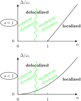
Figure 1: Sketch of the generic phase diagram of the spin-boson model, in the ohmic ($s=1$) and sub-ohmic ($0<s<1$) cases respectively, as a function of the dissipation parameter $\alpha$ and the dimensionless magnetic field $\Delta/\omega_{c}$. The super-ohmic ($s>1$) regime shows only the crossover from coherent to incoherent dynamics, without a localization transition. In all cases, the coherent/incoherent crossover happens at comparable coupling strength, namely $\alpha\simeq 0.5$.

In contrast, the sub-ohmic model ($0<s<1$) can undergo localization before or after the disappearance of the coherent oscillations, depending on the precise values of the microscopic parameters, Anders2 ; Thorwart see Fig. 1. In particular, in the limit of small magnetic field $\Delta/\omega_{c}\ll 1$, the quantum phase transition occurs at small dissipation $\alpha\ll 1$, so that low-energy dynamics (related to quantum criticality) and high energy physics (the damping of the Rabi oscillations) are governed by different energy scales, and both can be treated in principle by perturbative methods. We will focus in this section on a Numerical renormalization group (NRG) solution that encompasses both weak ($\alpha\ll 1$) and non-perturbative dissipation ($\alpha\simeq 0.1$) regimes, before making comparison with analytical methods in Sections III and IV for the weak dissipation case.

II.2 Bosonic NRG algorithm

The implementation of the NRG method follows the standard procedure initially introduced for fermionic models, Wilson ; BullaRMP and recently extended to bosonic Hamiltonians. Tong First, the spin-boson model (1) is rewritten in a continuous form:

$$H=\frac{\Delta}{2}\sigma^{x}+\frac{1}{2}\sigma^{z}\int_{0}^{\omega_{c}}\!\!\!\!\!d\epsilon\;h(\epsilon)\;[a^{\dagger}_{\epsilon}+a^{\phantom{\dagger}}_{\epsilon}]+\int_{0}^{\omega_{c}}\!\!\!\!\!d\epsilon\;\epsilon\;a^{\dagger}_{\epsilon}a^{\phantom{\dagger}}_{\epsilon}$$ (3)

with $J(\epsilon)/\pi=[h(\epsilon)]^{2}$. The bosonic bath $J(\epsilon)$ is then logarithmically discretized using the Wilson parameter $\Lambda>1$, first on the highest energy interval near the cutoff $[\Lambda^{-z}\omega_{c},\omega_{c}]$, and then iteratively on successive decreasing energy windows $[\omega_{n+1},\omega_{n}]$ with $\omega_{n}=\Lambda^{-n-z+1}\omega_{c}$ (for $n$ strictly positive integer). This choice of discretization introduces the so-called $z$-parameter (with $0<z\leq 1$) that is used to average over $N_{z}$ different realizations of the Wilson chain Oliveira1 (this amounts to gradual changes of boundary conditions, allowing to obtain better statistics from the numerical simulations). Taking $N_{z}$ different $z$ values, usually uniformly distributed in the $]0,1]$ interval, allows to obtain an order $N_{z}$ improvement of the spectral resolution at finite energy. For very narrow spectral structures in the correlation functions, this method becomes too expensive and and one lays recourse to improved broadening techniques, see Ref. Freyn, and Sec. II.3.

The bosonic fields are then decomposed in Fourier modes (with $p$ a positive or negative integer) on each interval $\omega_{n+1}<\epsilon<\omega_{n}$ of width $d_{n}=(1-\Lambda^{-1})\Lambda^{-n-z}$ for $n>0$ (note that $d_{0}=1-\Lambda^{-1}$):

$$a^{\dagger}_{\epsilon}=\sum_{n,p}\frac{e^{i2\pi p\epsilon/d_{n}}}{\sqrt{d_{n}}}\,a^{\dagger}_{n,p}.$$ (4)

This step is of course exact, and the first NRG approximation consists in neglecting all $p\neq 0$ modes, keeping only the operator $a^{\dagger}_{n}\equiv a^{\dagger}_{n,0}$ (the full Hamiltonian is thus only recovered in the $\Lambda\to 1$ limit. Bulla ) This leads to the “star”-Hamiltonian:

$$H_{\mathrm{star}}=\frac{\Delta}{2}\sigma^{x}+\frac{1}{2}\sigma^{z}\sum_{n=0}^{+\infty}\frac{\gamma_{n}}{\sqrt{\pi}}[a^{\dagger}_{n}+a^{\phantom{\dagger}}_{n}]+\sum_{n=0}^{+\infty}\xi_{n}a^{\dagger}_{n}a^{\phantom{\dagger}}_{n}$$ (5)

with the “impurity” coupling strength (the expressions below apply for $n>0$ only, the $n=0$ value can be obtained analogously)

$$\gamma_{n}^{2}=\int_{\omega_{n+1}}^{\omega_{n}}\!\!\!\!d\omega\,J(\omega)=2\pi\alpha\frac{1-\Lambda^{-(s+1)}}{s+1}\omega_{c}^{2}\Lambda^{-(n+z)(s+1)}$$ (6)

and the typical energy $\xi_{n}$ in each Wilson shell

$$\xi_{n}=\frac{1}{\gamma_{n}^{2}}\int_{\omega_{n+1}}^{\omega_{n}}\!\!\!\!d\omega\,\omega\,J(\omega)=\frac{s+1}{s+2}\frac{1-\Lambda^{-(s+2)}}{1-\Lambda^{-(s+1)}}\omega_{c}\Lambda^{-n-z}.$$ (7)

One then performs an exact mapping onto the so-called chain Hamiltonian:

$$H_{\mathrm{chain}} = \frac{\Delta}{2}\sigma^{x}+\frac{1}{2}\sigma^{z}\frac{\eta_{0}}{\pi}[b^{\dagger}_{0}+b^{\phantom{\dagger}}_{0}]$$

$$+\sum_{n=0}^{+\infty}[\epsilon_{n}b^{\dagger}_{n}b^{\phantom{\dagger}}_{n}+t_{n}(b^{\dagger}_{n+1}b^{\phantom{\dagger}}_{n}+b^{\dagger}_{n}b^{\phantom{\dagger}}_{n+1})]$$

where $\eta_{0}=\int d\epsilon J(\epsilon)$ and the on-site energies $\epsilon_{n}$ and intersite hoppings $t_{n}$ are determined numerically by a tridiagonalization of the bosonic part of the star Hamiltonian (5).

The remaining step of the NRG follows Ref. Tong, , adding successively sites into $H_{\mathrm{chain}}$ starting with $n=0$. The site of order $n$ roughly describes the physics for energies of the order $\omega_{c}\Lambda^{-n}$. This iterative procedure allows to reach exponentially small scales in a linear effort, an important achievement for the study of Kondo physics Wilson or impurity quantum critical behavior. VojtaReview It is important to stress that the success of the NRG relies on the exponential decrease of the chain parameters $\epsilon_{n}$ and $t_{n}$ (related to the analogous behavior of the star parameters $\xi_{n}$ and $\gamma_{n}$), which makes the iterative diagonalization reliable and stable (see however Ref. Freyn2, for the extension of NRG to other classes of models). Because the size of the Hilbert space needs to remain finite, truncation constraints need to be implemented. Typical calculations are usually performed with $N_{b}=10$ bosonic states on each successive bosonic site of the Wilson chain that is added during the renormalization procedure, Tong ; Freyn and $N=160$ kept NRG states (truncation). Matrix sizes thus do not exceed $2000\times 2000$ during the whole computation, and we proceed to $N=30$ NRG iterations with $\Lambda=2$ , so that a typical low energy scale $\omega_{\mathrm{min}}=\omega_{c}\Lambda^{-N}\simeq 10^{-9}$ can be reached. The resulting discrete energy spectra at successive NRG iterations are combined using the interpolation scheme proposed in Ref. Bulla3, (see however the more rigorous implementation given by full density-matrix NRG calculations Weichselbaum ; Peters ), leading to a set of $z$-dependent many-body energy levels $\epsilon_{k,z}$ labelled by quantum number $k$. The spin-spin correlation function along the $i$-axis ($i=x,y,z$) is defined from the equilibrium spin autocorrelation functions in real time and their Fourier transform to real frequency:

$$C_{i}(t) = \frac{1}{2}\big{<}[\sigma_{i}(t),\sigma_{i}(0)]\big{>}$$ (9)

$$C_{i}(\omega) = \int\frac{\mathrm{d}\omega}{2\pi}\,C_{i}(t)\cos(\omega t).$$ (10)

An alternative way to introduce the spin dynamics is from the imaginary time spin correlation functions and their Fourier transform onto Matsubara frequency:

$$\chi(\tau) = \big{<}S_{i}(\tau)S_{i}(0)\big{>}$$ (11)

$$\chi(i\nu) = \int_{0}^{\beta}\!\!d\tau\,e^{i\nu\tau}\chi(\tau)$$ (12)

$$\chi(\omega+i0^{+}) = \chi^{\prime}(\omega)+i\chi^{\prime\prime}(\omega)$$ (13)

where analytic continuation was performed in the last equation in order to obtain the retarded spin susceptibility. These susceptibilities are simply related to the spin autocorrelation functions (10) by the fluctuation-dissipation theorem, which reads at equilibrium and for zero temperature (we consider the $T=0$ limit in all what follows):

$$C_{i}(\omega) = \mathrm{Sign}(\omega)\chi_{i}^{\prime\prime}(\omega).$$ (14)

We will therefore use equivalently both nomenclatures in the rest of the paper. There exists an important equation, known as Shiba’s relation, Costi ; Tong which connects real and imaginary parts of the spin susceptibility at low frequency. This exact relation is usually derived for the ohmic ($s=1$) spin-boson model (or equivalently for the anisotropic Kondo model) and reads at small frequency:

$$C_{z}(\omega)=2\pi\alpha|\omega|[\chi^{\prime}_{z}(0)]^{2}.$$ (15)

We will prove in appendix A that this result can be generalized to the sub-ohmic case ($0<s<1$) in the following form

$$C_{z}(\omega)=J(|\omega|)[\chi^{\prime}_{z}(0)]^{2}$$ (16)

valid in the small $\omega$ limit. An useful byproduct of Shiba’s relation is that, at a magnetic ordering of the spin (corresponding to the quantum critical point), the susceptibility $\chi^{\prime}_{z}(0)$ diverges, so that the low-energy power law behavior $C_{z}(\omega)\propto J(|\omega|)\propto|\omega|^{s}$ obeyed in the whole delocalized phase should turn into a different (and diverging) power law.

A last important technical step is that all these correlation functions can be computed at zero temperature from the raw NRG data using Lehmann’s decomposition rule:

$$C_{i}(\omega)=\frac{1}{2N_{z}}\sum_{k,z}|\langle 0,z|\sigma_{i}|k,z\rangle|^{2}\delta\left(|\omega|+\epsilon_{0,z}-\epsilon_{k,z}\right)$$ (17)

where $\epsilon_{0,z}$ is the ground state energy. This leads to a superposition of sharp $\delta$-peaks which need to be broadened. This sensitive issue is examined now.

II.3 Optimized broadening method

A single NRG calculation (for a given value of $z$) usually provides a set of energy levels which come by packets located around each Wilson shell. The energy resolution at scale $\omega_{n}=\Lambda^{-n-z}$ is thus usually thought to be of the order $d_{n}=\omega_{n}-\omega_{n+1}=(1-\Lambda^{-1})\omega_{n}$, and degrades at higher energy. In order to generate smooth NRG spectra, the delta-peaks in the Lehmann formula (17) are therefore usually broadened BullaRMP at energy $\omega_{n}$ on a scale of the same order (the broadening scale is typically $b\omega_{n}$, with $b\simeq 0.7$) using the substitution:

$$\delta\left(|\omega|-\omega_{n}\right)\rightarrow\frac{e^{-b^{2}/4}}{\omega_{n}b\sqrt{\pi}}e^{-[\log(|\omega|/\omega_{n})^{2}/b]^{2}}.$$ (18)

As a result, spectral features at a given energy $\omega$ that are sharper than $\omega$ itself cannot be well resolved, and will come out overbroadened. Some relative degree of improvement can be achieved by combining $N_{z}$ NRG runs with different values of the $z$ parameter ($z$-averaging procedure, or $z$-trick Oliveira1 ). Although the mathematical justification for this procedure is still unclear, in the optimal case the resulting energy packets turn out to be uniformly distributed if the set of $z$-values is also chosen uniformly, and this allows a decrease of the broadening parameter to $b\simeq 0.7/N_{z}$. In the case of very sharp features, this method requires a large number of NRG runs, and will be prohibitive. It may also become problematic in regions where the $z$-averaging does not provide a uniform distribution of states (this may occur from the accidental disappearance of some NRG states), in which case uncontrolled oscillations of period $\Lambda$ can be generated (situation of underbroadening). These problems have led authors to speculate that quantitative NRG spectral functions can be extracted only in the continuum limit, Zitko ; Oliveira2 ; Weichselbaum2 either with $\Lambda\rightarrow 1$ or $N_{z}\rightarrow+\infty$ (only the former is mathematically sound, but the NRG algorithm cannot be managed anymore as scale separation breaks down). Both limitations of the $z$-averaging can however be lifted thanks to a simple remark made by two of us in a previous publication: Freyn for a single NRG run, the levels within a given logarithmic energy window are not uniformly distributed, but rather tend to bunch together close to sharp resonances. This effect becomes quite obvious when the width of such resonance becomes extremely small, see Fig. 2, but is always present in all NRG calculations.

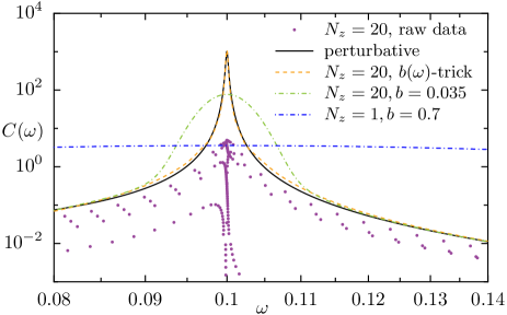
Figure 2: (Color online) The transverse (along the bath) spin susceptibility $C_{z}(\omega)$ of the sub-ohmic spin-boson model at $s=0.1$, $\Delta=0.1\omega_{c}$ and $\alpha=0.000125$. Raw data $|\langle 0,z|\sigma_{z}|k,z\rangle|^{2}/[2N_{z}(\epsilon_{k,z}-\epsilon_{0,z})]$ are given as circles for $N_{z}=20$ combined NRG calculations, solid line is the perturbative result, and the three dashed lines are the various NRG broadenings discussed in the text. All frequency-dependent plots are given in units of $\omega_{c}=1$.

Figure  2 shows indeed the raw NRG spectra for one of the spin susceptibilities of the spin-boson model, computed with $N_{z}=20$ interleaved $z$-averaged NRG runs (dots) and smoothed using two standard NRG broadenings (dash-dotted curves) with respective parameters $b=0.7$ and $b=0.7/N_{z}=0.035$. The largest broadening clearly fails to produce the expected peak (as a testbed, an accurate analytical expression is provided by the full line, see Sec. III for further details), while the smallest broadening signals the peak, but overestimates its width by more than one order of magnitude! Large scale $z$-averaging with $N_{z}\simeq 10^{4}$ would probably allow to resolve the correct spectral structure, but is unreasonably expensive. The key observation Freyn is that the NRG eigenvalues do not always come in packets uniformly distributed within the Wilson shell, but on the contrary tend to cluster close to resonances, as clearly seen on the raw data (dots) in Fig. 2. This provides the missing information which is needed in order to achieve a good spectral resolution with a limited numerical cost. The main strategy to be used is that the broadening parameter $b$ must become energy-dependent, which we previously called the “b-trick”. Freyn However, the generic implementation of this simple idea is not fully clarified: we present here a simple scheme that seems to be quite efficient, but we emphasize that a more generic and robust method is still to be found. The required algorithm must indeed adapt the broadening parameter $b(\omega)$ in Eq. (18) to the frequency dependence of the density of highest weight NRG peaks. Our approach, which draws inspiration from the NRG logarithmic discretization, is to extract $b(\omega)$ from the logarithmic derivative of the integrated spectrum up to frequency $\omega$:

$$b(\omega)=\frac{b_{0}}{2}\left(\left[q+\frac{{{\mathrm{d}}}\log\int_{0}^{\omega}C}{{{\mathrm{d}}}\log\omega}\right]^{-1}\!\!\!\!\!\!+\!\left[q+\frac{{{\mathrm{d}}}\log\int_{+\infty}^{\omega}C}{{{\mathrm{d}}}\log\omega}\right]^{-1}\right)$$ (19)

where $q\simeq 1$ is a regularization parameter whose precise value does not matter much to the final result, and $b_{0}$ provides the typical broadening at low and high frequencies (far from the atomic resonances). Note that we have used here two different frequency sweeps, one from $\omega=0$ and one from $\omega=+\infty$, in order to treat on an equal basis low and high frequency tails (this procedure is not satisfactory in cases where several resonances are present). Because the actual NRG data is fully discrete, see Eq. (17), we compute $b(\omega)$ recursively using Eq. (19) on the broadened NRG spectra. This procedure converges after few iterations to the results displayed on Fig. 2. It is clearly remarkable that such a good agreement can be reached with so little numerical effort, demonstrating that the raw NRG data encode much more information than previously thought (see Ref. Freyn, for further details). One important advantage of the b-trick is that $b(\omega)$ takes very small values near resonances, greatly enhancing the resolution, while keeping large values away from the peak, thus avoiding the usual underbroadened NRG oscillations. The main tuning parameter in our method is the low-frequency broadening $b_{0}$ in Eq. (19), which is determined by a simple convergence method. We finally emphasize that some degree of z-averaging is always needed in order to generate smooth spectra with the b-trick, but in our experience z-averaging alone is never sufficient to obtain accurate results near sharp finite-frequency resonances.

II.4 NRG results for the dynamical susceptibilities in the three spin directions

We present here the NRG data for a fixed value of the magnetic field $\Delta/\omega_{c}=0.1$, varying the dissipation from values $\alpha\ll\alpha_{c}$ (far from the quantum critical point) up to $\alpha_{c}$. We choose three different values of the bath exponent $s=0.1,0.5,1.0$, which span the complete generality of the model. We remark that the case $s=0$ is special, as the spin is localized for all $\alpha>0$ at zero temperature Anders2 , and will not be considered here, as we aim at understanding the delocalized phase of the model only. We will also not examine the situation of $s>1$, which shows for weak dissipation similar features as the $s=1$ case, and does not present a phase transition at larger coupling. We stress already that depending whether $\alpha_{c}\ll 1$ or not, the transition will or won’t take place at weak coupling, and this can lead to different physical pictures.

Let us consider first the case $s=0.1$ and the spin susceptibilities along each spin direction ($i=x,y,z$) shown in Fig. 3 (the plot also includes a comparison to lowest order pertubation theory, introduced in Section III.2).

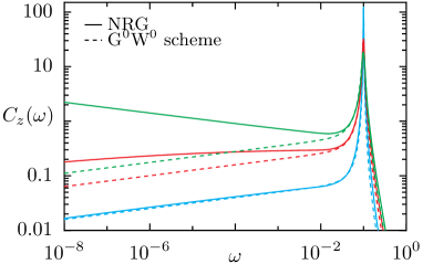
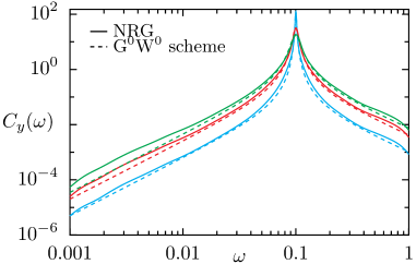
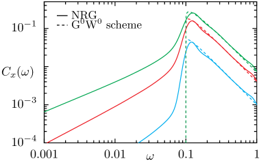
Figure 3: Spin susceptibilities $C_{z}(\omega)$, $C_{y}(\omega)$ and $C_{x}(\omega)$ (top to bottom panels) for $\Delta/\omega_{c}=0.1$, $s=0.1$ and increasing dissipation strength $\alpha=0.001,0.004,0.007$ (bottom to top). The critical point is located at $\alpha_{c}\simeq 0.007$. The NRG plots were generated with $N_{z}=20$ interleaved z-averages and used the b-trick discussed in Sec. II.3, while the perturbative expressions (G⁰W⁰ scheme) are given in Eqs. (36-37). Note that the upper panel has a different range in $\omega$ than the two other panels.

The transverse (orthogonal to the field and parallel to the bath) spin susceptibility $C_{z}(\omega)$, already considered, Anders2 ; Freyn shows two interesting features. First, the resonance at $\omega=\Delta$ broadened by the bath is always sharply defined, because here $\alpha_{c}\simeq 0.007$ is so small that one remains in the perturbative regime for all $\alpha<\alpha_{c}$ values regarding this high energy features. This is consistent with the near perfect agreement with the perturbative result in this range of frequencies, and weakly damped oscillation should occur in the real-time spin dynamics. The low-energy part of this spectral function is yet more interesting. For $\alpha\ll\alpha_{c}$, a slow decay with $C_{z}(\omega)\propto|\omega|^{s}$ is observed, also consistent with the perturbative result. Increasing $\alpha$, a crossover at a scale $\omega^{\star}$ is seen between the $|\omega|^{s}$ behavior at $\omega\ll\omega^{\star}$ and a different power law $|\omega|^{-s}$ at $\omega^{\star}\ll\omega\ll\Delta$. At the quantum critical point $\alpha=\alpha_{c}$, $\omega^{\star}$ vanishes and a complete $|\omega|^{-s}$ divergence is realized throughout. Clearly, the perturbative expression fails to reproduce this behavior. We stress here that even values relatively far from the critical point, such as $\alpha=0.004$, show large quantitative deviation from lowest order perturbation theory at low frequency, despite the good agreement on the coherent peak. This shows that the range of validity of perturbative methods (such as Bloch-Redfield), although possibly accurate at short time scales, is very limited in the long time limit. Clearly the high energy dissipation mechanism does not care for the complex low-energy behavior of the spin dynamics, even at the quantum critical point. Tong ; Anders Turning to the second transverse susceptibility $C_{y}(\omega)$ (orthogonal to both the magnetic field and the spin-bath term), we observe similar behavior as in $C_{z}(\omega)$ for the resonant peak, and good agreement with perturbation theory. The low energy part of the spectrum is however much less dramatic, because critical modes, related to fluctuations driven by the bath, pertain mainly to the $z$-component of the spin. What is actually going on is a very mild crossover from $\omega^{2+s}$ at $\omega\ll\omega^{\star}$ to $\omega^{2-s}$ at $\omega^{\star}\ll\omega\ll\Delta$ (the latter behavior includes the whole range of low frequencies at the critical point), due to the small value of $s=0.1$. Agreement with perturbation theory appears thus much better, although small deviations, due to the tiny changes of the power law exponent, can be seen at low frequency. These precise (and exact) values for the various power laws will be demonstrated in Section III. Finally, the longitudinal (parallel to the bath) spin susceptibility $C_{x}(\omega)$ presents quite different features. Clearly in the absence of dissipation ($\alpha=0$), a $\delta(\omega)$ peak at zero frequency occurs, in contrast to the $\delta(\omega-\Delta)$ peak at the magnetic field frequency displayed by both $C_{y}(\omega)$ and $C_{z}(\omega)$. Thus no sharp resonance is generated at small dissipation, and rather a broad shoulder emerges, quite reminiscent of the T-matrix of the Kondo model in a magnetic field. Paaske This structure is well accounted for by the perturbative calculation for $\Delta<\omega$, however, stark discrepancy is seen at low frequency for $|\omega|<\Delta$: the NRG data present a tail of low energy modes, while perturbation theory provides a gap in this range. This new feature given by the NRG will be elucidated in Section III.3, in connection with multiparticle effects in the diagrammatics, that are neglected in the current lowest order calculation.

We now turn to the intermediate value of $s=0.5$, giving rise to a somewhat larger critical dissipation strength $\alpha_{c}\simeq 0.105$, see Fig. 4.

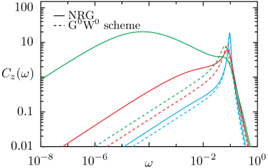
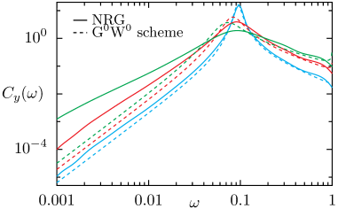
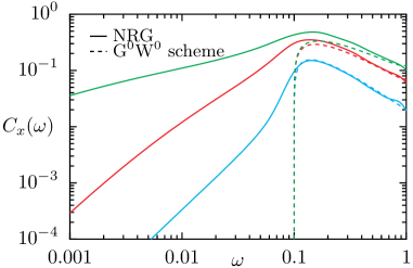
Figure 4: Spin susceptibilities $C_{z}(\omega)$, $C_{y}(\omega)$ and $C_{x}(\omega)$ (top to bottom panels) for $\Delta/\omega_{c}=0.1$, $s=0.5$ and increasing dissipation strength $\alpha=0.02,0.06,0.1$ (bottom to top). The critical point is located at $\alpha_{c}\simeq 0.105$. The NRG plots were generated with $N_{z}=10$ interleaved z-averages and used the b-trick discussed in Sec. II.3, while the perturbative expressions (G⁰W⁰ scheme) are given in Eqs. (36-37). Note that the upper panel has a different range in $\omega$ than the two other panels.

In that case, the smallest chosen value of $\alpha=0.02$ still lies in the perturbative regime, so that again near perfect agreement with perturbation theory can be checked. However, the approach to the quantum critical point shows larger quantitative deviations, both at high and low energy. Clearly, the coherent peak is more strongly smeared in the NRG for the larger shown values $\alpha=0.06,0.1$ compared to perturbation theory, due to the now relatively important magnitude of $\alpha$. Nevertheless, the peak structure survives up to the critical point, so that moderately damped oscillations should show up in the time domain, even close to $\alpha_{c}$. Regarding the low energy part of the spectrum, the same crossover from $\omega^{s}$ to $\omega^{-s}$ behavior (for $\omega\ll\omega^{\star}$ and $\omega^{\star}\ll\omega\ll\Delta$ respectively) is seen in $C_{z}(\omega)$, now more clearly defined due to the larger value of $s=0.5$. Again perturbation theory fails in this regime, and this is now more easily seen on $C_{y}(\omega)$ as well, which presents respectively a crossover from $\omega^{2+s}$ to $\omega^{2-s}$ in the frequency dependency. We note also a similar enhancement of the low energy tails for the last component $C_{x}(\omega)$ below the shoulder at $\omega<\Delta$.

We finally consider the so-called ohmic case $s=1$, for which $\alpha_{c}\simeq 1$, clearly out of the perturbative range, see Fig. 5.

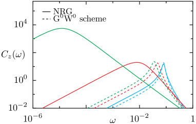
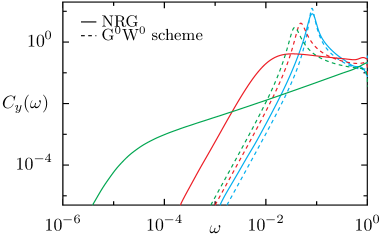
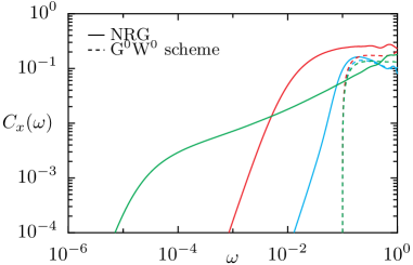
Figure 5: Spin susceptibilities $C_{z}(\omega)$, $C_{y}(\omega)$ and $C_{x}(\omega)$ (top to bottom panels) for $\Delta/\omega_{c}=0.1$, $s=1$ and increasing dissipation strength $\alpha=0.1,0.5,0.9$ (bottom to top). The critical point is located at $\alpha_{c}\simeq 1$. The NRG plots were generated with $N_{z}=3$ interleaved z-averages and used the b-trick discussed in Sec. II.3, while the perturbative expressions (G⁰W⁰ scheme) are given in Eqs. (36-37).

Again, small values of $\alpha=0.1$ present well-defined resonance and reasonable agreement with perturbation theory, although some deviations are visible. However, all values of $\alpha\gtrsim 0.5$ show a complete disappearance of the coherent peak at $\omega=\Delta$, leaving only the crossover scale $\omega^{\star}$, which separates regimes where $C_{z}(\omega)\propto\omega$ for $\omega\ll\omega^{\star}$ to $C_{z}(\omega)\propto\omega^{-1}$ (up to logarithmic corrections) for $\omega^{\star}\ll\omega\ll\omega_{c}$. In that case, oscillations are completely overdamped, and coherence is lost already well before the quantum critical point $\alpha_{c}=1$ where the spin becomes logarithmically free (this point corresponds precisely to the ferromagnetic scaling limit in the associated Kondo model). Again, $C_{y}(\omega)$ shows a similar behavior as observed for smaller $s$ values, with a crossover from $\omega^{2+s}=\omega^{3}$ to $\omega^{2-s}=\omega$ power laws for $\omega\ll\omega^{\star}$ and $\omega^{\star}\ll\omega\ll\Delta$ respectively. Finally $C_{z}(\omega)$ presents also a similar crossover in the low-energy tails, and a broad shoulder at the magnetic field value (for weak dissipation).

We now turn to the analytical description of this physics, and show that both qualitative and quantitative aspects of the numerical data can be well understood on the basis of the Majorana-fermion diagrammatic method.

III Majorana diagrammatics

III.1 Spin representation and correlation functions

The idea we henceforth develop is to use a Majorana description Maj1 ; Maj2 for the impurity quantum spin $\vec{S}=\frac{1}{2}\vec{\sigma}$, in order to capture quantitatively the spin fluctuations in the whole delocalized phase up to the quantum critical point using a weak dissipation expansion (understanding the quantum phase transition coming in from the localized phase is a more delicate issue, that we will not attempt here). Technically, our methodology involves the introduction of a triplet of real fermions $\eta_{j}$ (with $j=x,y,z$) that satisfy the anticommutation relations $\{\eta_{j},\eta_{k}\}=\delta_{jk}$, leading to the faithful representation $S_{j}=-(i/2)\sum_{kl}\epsilon_{jkl}\eta_{k}\eta_{l}$. We emphasize that Majorana qubits Hasan involve a doublet of real fermions, while the mathematical decomposition of a two-level qubits requires a triplet of real fermions. The main motivation behind considering the Majorana representation instead of more standard ones (Abrikosov or Popov fermions, Holstein-Primakoff or Schwinger bosons) is that one can alternatively write $\vec{S}=\chi\vec{\eta}$, where $\chi=-2i\eta_{x}\eta_{y}\eta_{z}$ is a fermionic operator which commutes with the Hamiltonian (1). This implies the crucial property that the spin susceptibilities Eq. (10) are obtained as simple identities involving standard one-particle Majorana Green’s function (here at zero temperature):

$$C_{i}(\omega)=-\frac{1}{\pi}\mathcal{I}m\,G_{i}(\omega),$$ (20)

where $G_{i}(\omega)$ is the retarded real-frequency Majorana-fermion Green’s function, obtained from the Fourier transformation of the time-ordered Green’s function $G_{i}(t)=-i\theta(t)\big{<}\{\eta_{i}(t),\eta_{i}(0)\}\big{>}$. This key relation between $C_{i}$ and $G_{i}$ is in great contrast to all other spin representations where the spin correlation functions are given in terms of four-fermion correlators, making the diagrammatics much more cumbersome. Therefore, thanks to Eq. (20), both the dissipative features at high energy and the low-energy quantum dynamics close to the quantum critical point can be simply encoded via Dyson equation by a Majorana-fermion self-energy. To obtain these important relations, we need to reexpress the spin-boson model Eq. (1) in the Majorana language:

$$H=-i\Delta\eta_{y}\eta_{z}-i\lambda\eta_{x}\eta_{y}\sum_{j}(a^{\dagger}_{j}+a^{\phantom{\dagger}}_{j})+\sum_{j}\omega_{i}a^{\dagger}_{j}a^{\phantom{\dagger}}_{j}.$$ (21)

The “diagonal” part given by the magnetic field is readily diagonalized into “free” (or bare) Majorana Green’s functions:

$$G_{x}^{0}(\omega) = \frac{1}{\omega+i0^{+}}$$ (22)

$$G_{y}^{0}(\omega) = \frac{\omega}{(\omega+i0^{+})^{2}-\Delta^{2}}$$ (23)

$$G_{z}^{0}(\omega) = \frac{\omega}{(\omega+i0^{+})^{2}-\Delta^{2}}$$ (24)

which are readily interpreted by a spin precession in the $y-z$ plane around the magnetic field pointing in the $x$ direction. Interaction between the Majorana fermions is generated by the coupling to the bosonic bath, which can be expressed as a bare vertex involving the $\eta_{x}$ and $\eta_{y}$ field, see Fig. 6.

Figure 6: Bare vertex of the spin-boson model in the Majorana language.

This coupling results in three Majorana self-energies $\Sigma_{i}(\omega)$, but clearly the $z$-component vanishes altogether, $\Sigma_{z}(\omega)=0$, due to the form of the interaction. Inverting the Majorana propagator (written in matrix form):

$$\hat{G}=\left[\begin{array}[]{ccc}\omega-\Sigma_{x}(\omega)&0&0\\ 0&\omega-\Sigma_{y}(\omega)&i\Delta\\ 0&-i\Delta&\omega\end{array}\right]^{-1}$$ (25)

provides Dyson’s equation for the full retarded Majorana Green’s functions that encode the complete spin dynamics:

$$G_{x}(\omega) = \frac{1}{\omega-\Sigma_{x}(\omega)}$$ (26)

$$G_{y}(\omega) = \frac{\omega}{\omega[\omega-\Sigma_{y}(\omega)]-\Delta^{2}}$$ (27)

$$G_{z}(\omega) = \frac{\omega-\Sigma_{y}(\omega)}{\omega[\omega-\Sigma_{y}(\omega)]-\Delta^{2}}$$ (28)

The bare Green’s functions (22-24) are correctly reproduced in the zero-dissipation limit, replacing $\Sigma_{i}(\omega)$ by a vanishing imaginary part $-i0^{+}$.

Because the interaction term in the Hamiltonian Eq. (21) involves a particular combination of the bosonic modes, it is useful to define the full bosonic propagator $G_{\Phi}(t)=-i\theta(t)\left<[\Phi(t),\Phi(0)]\right>$ of the “local” field $\Phi\equiv-i\frac{\lambda}{\sqrt{\alpha}}\sum_{j}(a^{\dagger}_{j}+a^{\phantom{\dagger}}_{j})$. This allows us to introduce a bosonic self-energy $\Sigma_{\Phi}(\omega)$ for the full Green’s function

$$G_{\Phi}(\omega)=\frac{G_{\Phi}^{0}(\omega)}{1-G_{\Phi}^{0}(\omega)\Sigma_{\Phi}(\omega)}$$ (29)

in terms of the bare bosonic propagator

$$G_{\Phi}^{0}(\omega)=\frac{1}{\alpha}\sum_{j}\left[\frac{\lambda^{2}}{\omega+i0^{+}-\omega_{j}}-\frac{\lambda^{2}}{\omega+i0^{+}+\omega_{j}}\right].$$ (30)

Using the convention chosen to normalize $\Phi$, the bare vertex takes simply the value $\sqrt{\alpha}$ (see Fig. 6), and the bare bosonic Green’s function can be expressed through the bosonic spectral density $J(\omega)$ given by Eq. (2):

$$G_{\Phi}^{0}(\omega) = -\frac{1}{\alpha}\int\frac{\mathrm{d}\epsilon}{\pi}\frac{J(|\epsilon|)\,\mathrm{Sign}(\epsilon)}{\omega+i0^{+}-\epsilon}$$ (31)

$$= -2\omega_{c}^{1-s}\int_{-\omega_{c}}^{\omega_{c}}\mathrm{d}\epsilon\,\frac{|\epsilon|^{s}\,\mathrm{Sign}(\epsilon)}{\omega+i0^{+}-\epsilon}$$

a quantity which is indeed independent of the dissipation strength $\alpha$, now encoded (by convention) only in the bare vertex. We thus find an explicit expression for the imaginary part of the bosonic Green’s function:

$$\mathcal{I}mG_{\Phi}^{0}(\omega)=2\pi\omega_{c}\mathrm{Sign}(\omega)\left|\frac{\omega}{\omega_{c}}\right|^{s}\theta(\omega_{c}^{2}-\omega^{2}).$$ (32)

The real part of the integral (31) can be computed analytically from Kramers-Kronig’s relation only in the low-energy limit $|\omega|\ll\omega_{c}$:

$$\mathcal{R}eG_{\Phi}^{0}(\omega)=\frac{4\omega_{c}}{s}-2\pi\omega_{c}\mathrm{cotan}\left(\frac{\pi s}{2}\right)\left|\frac{\omega}{\omega_{c}}\right|^{s}$$ (33)

although the complete formula (31) will be used for later numerical computations. The low-energy expression (33) breaks down for $s=1$, where additional logarithmic corrections arise (hinting at the known connection to the Kondo model Leggett ).

The exact resummation of perturbation theory requires the accurate knowledge of the full fermionic and bosonic self-energies, as well as the full three-particle vertex $\Gamma$ (a quantity that depends on three independent external frequencies). The general diagrammatics is given formally in Fig. 7.

Figure 7: Exact formal diagrammatic expression for the fermionic and bosonic self-energies in terms of the full (exact) fermionic and bosonic Green’s functions ($G_{i}$ and $G_{\Phi}$ respectively) and the full (exact) three-particle vertex $\Gamma$.

We note that replacement of the bare propagators by the full ones without considering together the vertex corrections must be done in general with care, and can lead to serious pathologies, see Ref. Vignale, . An exception to this rule is given in Sec. III.3, and the precise role of the interaction vertex will be elucidated in Sec. IV.5.

III.2 Lowest order perturbative self-energies in the Majorana diagrammatics

For very weak dissipation $\alpha\ll 1$ and far from the quantum critical point $\alpha\ll\alpha_{c}$, the spin dynamics should in principle be well described by the lowest order perturbative Majorana self-energies (we will see in Sec. III.3 that this naive statement is not completely correct in some specific frequency range). These self-energies are obtained at order $\alpha$ by a single boson exchange, see Fig. 8, where both fermionic and bosonic lines are given by the bare propagators Eqs. (22-24) and Eq. (31), respectively. In terms of resummation of diagrams, this level of approximation corresponds to the so-called $G^{0}W^{0}$ scheme for the generic fermion-boson models arising in the fields of heavy fermions Hertz or strongly interacting electron liquids Vignale ($G^{0}$ denotes the bare fermionic propagator and $W^{0}\equiv G_{\Phi}^{0}$ the bare bosonic one). It is alternatively called the (non-self-consistent) Born approximation in the context of disordered systems, DiCastro and it roughly corresponds to the weak-coupling Bloch-Redfield approximation for the real-time non-equilibrium dynamics of the spin-boson model. Shnirman Note that the present Majorana diagrammatics is formulated for the equilibrium dynamics only. Extension to temporal dynamics under a sudden switching (of the bath or transverse field) could be incorporated in our formalism by using two-times Keldysh Majorana Green’s functions, which lies however beyond the scope of the present work.

Figure 8: Lowest order perturbative Majorana self-energies, obtained from bare fermion and bare bosonic propagators ($G^{0}W^{0}$ scheme).

Standard evaluation of the diagrams provides the following imaginary part of the Majorana self-energies at zero temperature:

$$\mathcal{I}m\Sigma_{x}^{G^{0}W^{0}}\!(\omega) = \alpha\int_{0}^{\omega}\!\!\frac{\mathrm{d}\epsilon}{\pi}\mathcal{I}mG_{y}^{0}(\epsilon)\mathcal{I}mG_{\Phi}^{0}(\omega-\epsilon)$$ (34)

$$\mathcal{I}m\Sigma_{y}^{G^{0}W^{0}}\!(\omega) = \alpha\int_{0}^{\omega}\!\!\frac{\mathrm{d}\epsilon}{\pi}\mathcal{I}mG_{x}^{0}(\epsilon)\mathcal{I}mG_{\Phi}^{0}(\omega-\epsilon)$$ (35)

Using the bare propagators (22-24) and (30), one readily obtains:

$$\mathcal{I}m\Sigma_{x}^{G^{0}W^{0}}(\omega) = -\pi\alpha\omega_{c}\theta[\omega_{c}^{2}-(|\omega|-\Delta)^{2}]\theta(\omega^{2}-\Delta^{2})$$ (36)

$$\times\frac{||\omega|-\Delta|^{s}}{\omega_{c}^{s}}$$

$$\mathcal{I}m\Sigma_{y}^{G^{0}W^{0}}(\omega) = -\pi\alpha\omega_{c}\theta(\omega_{c}^{2}-\omega^{2})\frac{|\omega|^{s}}{\omega_{c}^{s}}$$ (37)

We are now equipped to start understanding the NRG results discussed in Section II.4. Owing to the general relation Eq. (20) between spin autocorrelation functions and Majorana propagators, we restrict the discussion to the latter in the rest of the paper. For $\alpha\ll 1$ one can safely neglect the small real part of the self-energy (corresponding to a tiny Knight shift of the spin precession frequency $\Delta$), so that we get from Dyson’s equations (26-28) for $|\omega|<\omega_{c}$:

$$\mathcal{I}mG_{x}^{G^{0}W^{0}}(\omega) \simeq -\frac{\pi\alpha\omega_{c}^{1-s}}{\omega^{2}}||\omega|-\Delta|^{s}\theta(\omega^{2}-\Delta^{2})$$ (38)

$$\mathcal{I}mG_{y}^{G^{0}W^{0}}(\omega) \simeq -\frac{\pi\alpha\omega_{c}^{1-s}|\omega|^{2+s}}{(\omega^{2}-\Delta^{2})^{2}+\omega^{2}\left[\pi\alpha\omega_{c}^{1-s}|\omega|^{s}\right]}$$ (39)

$$\mathcal{I}mG_{z}^{G^{0}W^{0}}(\omega) \simeq -\frac{\pi\alpha\omega_{c}^{1-s}\Delta^{2}|\omega|^{s}}{(\omega^{2}-\Delta^{2})^{2}+\omega^{2}\left[\pi\alpha\omega_{c}^{1-s}|\omega|^{s}\right]}$$ (40)

Following the discussion given in Sec. II.4, we start by interpreting the transverse susceptibilities $\mathcal{I}mG_{y}^{G^{0}W^{0}}$ and $\mathcal{I}mG_{z}^{G^{0}W^{0}}$. Clearly the $\delta(\omega-\Delta)$ peak is replaced by a sharp resonance, due to the small but finite lifetime given by $\mathcal{I}m\Sigma_{y}(\omega\simeq\Delta)$ in both expressions (39-40). The low-energy behavior is however different in those two quantities, as we find $\mathcal{I}mG_{y}^{G^{0}W^{0}}\propto|\omega|^{2+s}$ and $\mathcal{I}mG_{z}^{G^{0}W^{0}}\propto|\omega|^{s}$, in agreement with the NRG results, see the two topmost panels in Figs. 3-5 and the related discussion in Sec. II.4. A higher density of low-energy modes is indeed obtained in $C_{z}$ than in $C_{y}$, due to the coupling of the bosonic continuum to the spin along the $z$-axis. This leads therefore to the following decay of the $z$-component of the spin autocorrelation function $C_{z}(t)\propto 1/t^{1+s}$ in the long-time limit. In the perturbative regime $\alpha\ll 1$ and $\alpha\ll\alpha_{c}$, it is not surprising to find very accurate agreement between the NRG and our analytical expressions (note that the real parts of the self-energies have been included in all plots). Turning to the longitudinal susceptibility $\mathcal{I}mG_{x}^{G^{0}W^{0}}$, we observe in Eq. (38) a broad shoulder for $|\omega|>\Delta$, which is also seen in the numerics, but we obtain instead a hard gap in the range $|\omega|<\Delta$, in disagreement with the NRG data. This surprising failure of the perturbative method for $G_{x}^{G^{0}W^{0}}$ at weak dissipation comes from multiparticle effects beyond leading order, which do play a qualitative role whenever the spectral density is identically zero at lowest order in perturbation theory (otherwise higher order self-energy corrections are always small at weak coupling). We now examine this question in greater detail.

III.3 Multiparticle effects

We still consider here the spin dynamics at very weak dissipation $\alpha\ll 1$ and $\alpha\ll\alpha_{c}$, with the goal to improve the diagrammatics for the the lowest order longitudinal susceptibility $\mathcal{I}mG_{x}^{G^{0}W^{0}}$, whose spectrum is spuriously gapped at lowest order in perturbation theory. This inconsistency can be easily tracked to expression (22), where the bare transverse propagator $G_{y}^{0}$ resumes to a $\delta(|\omega|-\Delta)$ peak and misses the $\omega^{2+s}$ low-energy modes obtained from the coupling to the bosonic bath, see equation (39). The discrepancy is thus resolved by reinjecting the full Majorana-Green’s functions $G_{i}$ into the Majorana self-energies (this is the so-called $GW^{0}$ scheme, see Fig. 9):

$$\mathcal{I}m\Sigma_{x}^{GW^{0}}(\omega) = \alpha\int_{0}^{\omega}\frac{\mathrm{d}\epsilon}{\pi}\mathcal{I}mG_{y}(\epsilon)\mathcal{I}mG_{\Phi}^{0}(\omega-\epsilon)$$ (41)

$$\mathcal{I}m\Sigma_{y}^{GW^{0}}(\omega) = \alpha\int_{0}^{\omega}\frac{\mathrm{d}\epsilon}{\pi}\mathcal{I}mG_{x}(\epsilon)\mathcal{I}mG_{\Phi}^{0}(\omega-\epsilon)$$ (42)

Figure 9: Selfconsistent fermionic self-energies (analogous to the $GW^{0}$ approximation), allowing to improve the calculation in frequency ranges where lowest order perturbation incorrectly predicts the absence of spin excitations. This scheme recovers multiparticle excitations that fill in the spurious gaps of bare perturbation theory.

The low-energy tails of the transverse susceptibility will therefore fill in the gap of the longitudinal susceptibility, so that in principle a single iteration of the above self-consistent equation should be sufficient required. The results are shown in Fig. 10, demonstrating our correct physical interpretation of the missing low energy tails in $G_{x}$. We note that the two transverse susceptibilities are very mildly affected by the self-consistency at weak coupling, and were therefore not shown.

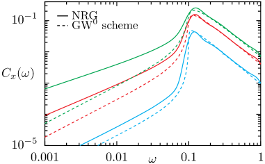
Figure 10: Longitudinal spin susceptibility $C_{x}(\omega)$ for $\Delta/\omega_{c}=0.1$, $s=0.1$ and $\alpha=0.001,0.004,0.007$ (bottom to top), comparing the NRG result to the self-consistent $GW^{0}$ scheme, allowing to recover the low-energy tail below the threshold $\omega=\Delta$ (results are quantitatively correct only for the smallest $\alpha$ value, see Sec. IV.5 for the improvements that are required near the quantum critical point).

A second instance where multiparticle effects are relevant occurs in the frequency range above the high energy cutoff, now for all three spin correlations. Indeed, lowest order perturbation theory provides again a gap for excitations with $|\omega|>\omega_{c}$, see Eqs. (36-37) in the case of one of the transverse spin correlation function (similar results are obtained for the other spin susceptibilities).

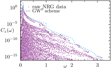
Figure 11: Transverse spin susceptibility $C_{z}(\omega)$ for $\Delta/\omega_{c}=0.1$, $s=0.1$ and $\alpha=0.002$, comparing the raw NRG data to the self-consistent $GW^{0}$ scheme. In contrast to bare perturbation theory, which leads to a gap for $\omega>\omega_{c}$, the self-consistent resummation correcly describes the tail arising from multiparticle excitations above the threshold $\omega_{c}$ (note the linear frequency scale).

In contrast, the NRG data show a tail with small yet non-zero spectral weight above the cutoff $\omega_{c}$, see Fig. 11. This continuum of magnetic excitations decays very quickly at increasing energy, and displays furthermore well-defined thresholds, pointing again to multiparticle effects, where more and more bosons are exchanged with the spin degrees of freedom, in agreement with recent observation. Nalbach Using the fermionic self-consistent scheme proposed in Eqs. (41-42), we indeed reproduce numerically both the rapidly decaying tail and the multiparticle thresholds at quantized values of the cutoff $\omega_{c}$ (we note that the multiparticle thresholds seen in the raw NRG data shift do not precisely match the quantized values, possibly an artifact of the discretization procedure). This final comparison concludes our study of the weak coupling regime $\alpha\ll\alpha_{c}$ of the spin-boson model.

IV Dynamics near the quantum critical point

IV.1 Role of the bosonic mass

We provide here general considerations on the structure of perturbation theory in terms of the coupled field theory of fermions and bosons, with the emphasis on the regime near the quantum critical point. The main motivation is to understand precisely where the singularities associated to critical modes will occur in the diagrammatics. From the knowledge gained in the previous weak coupling analysis, we understand that the fermionic sector is immune to singularities as long as the bosonic propagator remains regular. Clearly self-consistency for the fermionic self-energies ($GW^{0}$ scheme) provides only small perturbative correction and cannot account for critical behavior. One can convince oneself that the frequency-dependent vertex $\Gamma$ (see Fig. 7) is also regular as dissipation is increased. The only possibility left is that only the bosonic propagator encapsulates the singular dynamics via its self-energy (see general diagrammatic expression on the lower panel in Fig. 7). Indeed using the exact Dyson’s equation (29) and the asymptotic bare propagator (32-33), we get the low frequency retarded bosonic Green’s function:

$$G_{\Phi}(\omega) = \frac{1}{m_{\Phi}+[a+ib\mathrm{Sign}(\omega)]|\omega|^{s}-\Sigma_{\Phi}(\omega)+\Sigma_{\Phi}(0)}$$

$$m_{\Phi} = \frac{s}{4\omega_{c}}-\Sigma_{\Phi}(0)$$ (44)

with $m_{\Phi}$ the bosonic mass, $a$ and $b$ real coefficients that can be read from Eqs. (32-33). This simple expression allows to understand the development of critical fluctuations in the spin-boson model: the quantum critical point is just associated to a vanishing of the mass $m_{\Phi}$ in the denominator of the bosonic propagator, due to the progressive building up of the bosonic self-energy. At the quantum critical point, $\Sigma_{\Phi}(0)=s/(4\omega_{c})$, and the correlation function now diverges as $G_{\Phi}(\omega)\propto|\omega|^{-s}$ at low frequency, owing to expression (LABEL:critical). One can check that the frequency dependence of the bosonic self-energy $\Sigma_{\Phi}(\omega)$ is subdominant with respect to $\omega^{s}$ in all orders in perturbation theory, so that the $-s$ exponent of the critical fluctuations turns out to be exact. In contrast, the bosonic Green’s function has a non-divergent power law behavior at low frequency $G_{\Phi}(\omega)-G_{\Phi}(0)\propto|\omega|^{s}$ in the whole delocalized phase. This change of exponent near the quantum critical point can be used to explain the behavior of the transverse spin susceptibility, calculated previously with the NRG.

Figure 12: Fermionic self-energies (without self-consistency) including a dressed bosonic propagator (this is analogous to the $G^{0}W$ approximation). This scheme is necessary to recover the critical modes near the quantum critical point, but asks for a careful evaluation of the bosonic self-energy (see Fig. 13 and the related discussion in Sec. IV.2 and Sec. IV.4).

When using the full bosonic propagator within the fermionic self-energy (see Fig. 12), we get:

$$\mathcal{I}m\Sigma_{y}^{G^{0}W}(\omega) = -\frac{1}{2}\mathrm{Sign}(\omega)\mathcal{I}mG_{\Phi}(\omega)$$ (45)

$$\propto |\omega|^{-s}\;\;\mathrm{at}\;\;\alpha=\alpha_{c}$$ (46)

From the exact Dyson equation for the $\eta_{z}$ Majorana Green’s function Eq. (28), we then get at low frequency:

$$\mathcal{I}mG_{z}^{G^{0}W}(\omega) \simeq \frac{1}{\Delta^{2}}\mathcal{I}m\Sigma_{y}^{G^{0}W}(\omega)$$ (47)

$$\propto |\omega|^{-s}\;\;\mathrm{at}\;\;\alpha=\alpha_{c}$$ (48)

The divergence of the transverse spin susceptibility at the quantum critical point is thus explained (again, we stress that the above exponent is exact). Considering also the second transverse susceptibility Eq. (27), we get at low frequency:

$$\mathcal{I}mG_{y}^{G^{0}W}(\omega) \simeq \frac{\omega^{2}}{\Delta^{4}}\mathcal{I}m\Sigma_{y}^{G^{0}W}(\omega)$$ (49)

$$\propto |\omega|^{2-s}\;\;\mathrm{at}\;\;\alpha=\alpha_{c}$$ (50)

as also observed with the NRG calculations of Sec. II.4.

This discussion shows that even in the weak dissipation regime $\alpha\ll 1$, the presence of such critical modes for $\alpha\lesssim\alpha_{c}$ will invalidate bare perturbation theory. It is thus necessary to investigate in more detail the bosonic correlations, in order to improve the agreement between numerics and diagrammatic calculation. We start by an analytic computation of the bosonic self-energy up to two-loop order.

IV.2 Critical line at two-loop order

The lowest order (one-loop) contribution to the bosonic self-energy (first diagram in Fig. 13) is readily computed:

$$\Sigma_{\phi}^{\mathrm{1loop}}(\omega)=\frac{\alpha}{2\Delta}\frac{\Delta^{2}}{\Delta^{2}-(\omega+i0^{+})^{2}}.$$ (51)

This level of approximation in the diagrammatics is equivalent to the standard RPA for the interacting electron-gas. Vignale From vanishing of the mass in Eq. (44), the above result gives the critical dissipation at one-loop order

$$\alpha_{c}^{\mathrm{1loop}}=\frac{s}{2}\frac{\Delta}{\omega_{c}}+\mathcal{O}(s^{2}),$$ (52)

recovering previous results. Vojta We recognize here the multi-scale nature of the perturbative expansion in the dissipation strength. While the high-energy part of the spectrum is well described as long as $\alpha\ll 1$, the low energy sector will be immune to quantum critical fluctuations as long as $\alpha\ll\alpha_{c}$.

Figure 13: Diagrammatic representation for the bosonic self-energy computed up to two-loop order, leading to Eq. (53).

While $\alpha_{c}$ vanishes for $s\to 0$, showing that the quantum critical point is perturbatively accessible, the above result is only accurate for very small $s$. As we will demonstrate now, an anomalous power-law also shows up in the dependence of $\alpha_{c}$ with respect to the dimensionless parameter $\Delta/\omega_{c}$. To establish this result, we need to push the weak-coupling calculation of the bosonic mass to next to leading order (two-loops), see Fig. 13. After straigthforward but lengthy calculations, we find at zero frequency:

$$\Sigma_{\phi}^{\mathrm{2loop}}(0) = \frac{\alpha}{2\Delta}+\frac{\alpha^{2}}{4\Delta^{2}}\int_{0}^{+\infty}\!\!\frac{d\epsilon}{\pi}\,\mathcal{I}mG_{\Phi}^{0}(\epsilon)\,\frac{3\Delta+2\epsilon}{(\Delta+\epsilon)^{2}}$$ (53)

$$\simeq \frac{\alpha}{2\Delta}+\frac{\alpha^{2}}{s}\frac{\omega_{c}}{\Delta^{2}}\left[1-\left(1-\frac{s}{2}\right)\left(\frac{\Delta}{\omega_{c}}\right)^{s}\right]$$

where the last equation applies for $\Delta\lesssim\omega_{c}$. We now solve the equation $s/(4\omega_{c})=\Sigma_{\phi}^{\mathrm{1loop}}(0)+\Sigma_{\phi}^{\mathrm{2loop}}(0)$ determining the quantum critical point, which gives in the small $s$ limit:

$$\alpha_{c}^{\mathrm{2loop}}(\omega)=\frac{s}{2}\frac{\Delta}{\omega_{c}}\left[1+\frac{s}{2}-s\log\left(\frac{\Delta}{\omega_{c}}\right)\right]+\mathcal{O}(s^{3}).$$ (54)

This precise form confirms that the weak-coupling diagrammatics is controlled as a systematic small-$s$ expansion. The presence of a logarithmic correction hints for the following anomalous power-law behavior:

$$\alpha_{c}^{\mathrm{2loop}}(\omega)\simeq\frac{s}{2}\left(1+\frac{s}{2}\right)\left(\frac{\Delta}{\omega_{c}}\right)^{1-s}.$$ (55)

We will first examine this analytical result with respect to the NRG phase diagram, before turning to a more rigorous derivation.

IV.3 Phase diagram of the sub-ohmic spin-boson model

According to the above result, the formula (55) for the critical dissipation $\alpha_{c}$ remains perturbative either for small $s$ (at arbitrary $\Delta/\omega_{c}\lesssim 1$) or for small $\Delta/\omega_{c}$. In the latter limit, $s$ can take relatively large values, but should not be too close to 1, otherwise the small coefficient $(\Delta/\omega_{c})^{1-s}$ becomes of order 1, and perturbation theory breaks down. In this case, an alternative approach, based on a development at small $h\equiv\Delta/\omega_{c}$ but finite $\alpha$ can be put forward. Kosterlitz ; Bulla This results in the well-known one-loop scaling equations (which were initially obtained from the long-range unidimensional Ising model):

$$\frac{d\alpha}{dl} = (1-s)\alpha-\alpha h^{2}$$ (56)

$$\frac{dh}{dl} = (1-\alpha)h$$ (57)

where the parameter $l$ characterizes the change of scale during the renormalization procedure. We stress that these flow equations are valid for all values of $\alpha$, as long as $h\ll 1$, and are thus complementary to the regime of validity of our small $\alpha$ expansion at fixed $h$. Combining both equations, one obtains:

$$\frac{d}{dl}\left[\log(\alpha)-\alpha+\frac{h^{2}}{2}-(1-s)\log(h)\right]=0$$ (58)

From Eqs. (56) and (57) the renormalization fixed point occurs at $\alpha^{\ast}=1$ and $h^{\ast}=\sqrt{1-s}$ for $s\leq 1$, so that the critical line $\alpha_{c}(h)$ is obtained by the condition:

$$\log(\alpha_{c})+(1-\alpha_{c})+\frac{h^{2}-(1-s)}{2}-(1-s)\log\left(\frac{h}{\sqrt{1-s}}\right)=0$$ (59)

leading to the behavior $\alpha_{c}\propto h^{1-s}$ at $h\ll 1$ for all $s$. We also recover from this analysis the exact value $\alpha_{c}=1$ for $s=1$ in the $h\to 0$ limit.

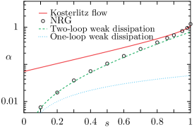
Figure 14: Phase diagram in the ($s$,$\alpha$) plane for $h\equiv\Delta/\omega_{c}=0.1$, comparing the NRG data to the Kosterlitz flow obtained from the resolution of Eq. (59) (giving reliable results for $0.9<s<1$), and to the one-loop and two-loop formulas (52) and (55) (the latter is accurate on the wide range $0<s<0.8$).

A joint comparison of the small $\alpha$ expansion and of the Kosterlitz flow to the NRG data is provided in Fig. 14 for the case $h=0.1$. While the two expansions work where they are expected to, the two-loop small $\alpha$-development is quantitatively accurate on the wide range $0<s<0.8$, while the one-loop small $h$-development is restricted to the small range $0.9<s<1$. Although pushing the small $h$ expansion to higher order would enhance the range of validity of the method, it is unlikely that this would recover the expected vanishing of $\alpha_{c}\simeq(s/2)h$ at small $s$. In contrast, the small $\alpha$-expansion converges very rapidly even for the largest $s$ values: the extreme case $s=1$ leads from Eq. (55) to the successive estimates $\alpha_{c}^{\mathrm{1loop}}=1/2$ and $\alpha_{c}^{\mathrm{2loop}}=3/4$ in the $\Delta/\omega_{c}\ll 1$ limit, approaching the exact value $\alpha_{c}=1$ in a steady fashion. As a clear illustration of this statement, we finally present in Fig. 15 a more systematic study of the phase diagram for several $h$ values, showing that the small $\alpha$ expansion remains accurate even at vanishing $h$, provided that $s<0.8$.

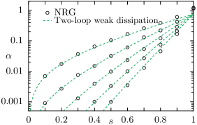
Figure 15: Phase diagram in the ($s$,$\alpha$) plane for $h\equiv\Delta/\omega_{c}=0.00001,0.0001,0.001,0.01,0.1$ (bottom to top), comparing the NRG simulations versus the two-loop weak dissipation result (valid for $s\ll 1$).

IV.4 Ladder resummation in the bosonic self-energy

We have just checked that our analytical expression for the critical dissipation (55) is in excellent agreement with the NRG data. However, the derivation of this result was performed by a strict expansion at two-loops, and a re-exponentiation of the logarithmically singular terms. In the spirit of a numerical scheme based only on Green’s functions, such as developed in Sec. III, the correct phase boundary will not be recovered if strict fourth order bosonic self-energies are used, and a clever resummation scheme should be found, that would be a diagrammatic equivalent to the re-exponentiation of the analytical result. Insight on this issue can be gained from the analytical derivation, because the logarithmic term in Eq. (54) can be traced back to a single diagram at two-loop order, namely the one with a single-rung ladder exchange in Fig. 13 (the last two diagrams with Majorana self-energy corrections are regular, and provide the perturbative corrections of order $s^{2}$ in Eq. (55)). This hints that the correct bosonic self-energy, and hence a quantitative phase diagram, will be obtained upon performing a ladder resummation to all orders, similar to the diffuson mode in disordered systems, DiCastro see Fig. 16.

Figure 16: Upper panel: ladder series for the bosonic self-energy that is needed to obtain the correct phase boundary within the diagrammatic calculation. Lower panel: single frequency approximation used at the two-rung level (and similarly for higher order contributions), see text.

Performing such calculation, even numerically, turns out to be difficult, because this requires the self-consistent determination of a four-electron vertex (depending of three independent external frequencies). A standard approximation in the field of disordered systems, DiCastro but also in the context of interacting electron liquids Vignale (called the Ng-Singwi scheme, or $GW_{\mathrm{eff}}$ approximation) amounts to keeping a single running frequency within the vertex, see lower panel of Fig. 16 in the case of a two-rung ladder. In our case, this approximation is vindicated by the fact that the low frequency part of the bosonic Green’s function provides the most important contribution to the Feynman diagram, so that strict energy conservation can be omitted from one rung to the next. We stress again that the inclusion of such vertex corrections in the fermionic self-energies are regular, and can be neglected at weak coupling, contrary to the singular bosonic propagator that we treat here. The ladder series including the full three particle vertex can now be explicitely carried out for the zero-temperature Matsubara bosonic self-energy:

$$\Sigma_{\Phi}^{\mathrm{ladder}}(i\nu)\simeq\alpha\int\frac{d\omega}{2\pi}G_{y}^{0}(i\omega+i\nu)G_{x}^{0}(-i\omega)\frac{1}{1-\Lambda^{0}(i\omega,i\nu)}$$ (60)

where

$$\Lambda^{0}(i\omega,i\nu)\simeq\alpha\int\frac{d\epsilon}{2\pi}G_{\Phi}^{0}(i\epsilon)G_{y}^{0}(-i\omega-i\epsilon)G_{x}^{0}(i\omega+i\nu+i\epsilon).$$ (61)

Evaluation of the zero-frequency self-energy can be carried out analytically in the small $\Delta/\omega_{c}$ limit, leading to:

$$\Sigma_{\Phi}^{\mathrm{ladder}}(0)=\frac{\alpha}{2\Delta}\frac{1}{1+\frac{2\alpha\omega_{c}}{s\Delta}\left[1-\left(\frac{\Delta}{\omega_{c}}\right)^{s}\right]}.$$ (62)

The phase boundary can now be obtained by solving $\Sigma_{\Phi}^{\mathrm{ladder}}(0)=1/G_{\Phi}^{0}(0)$, leading to the critical value $\alpha_{c}^{\mathrm{ladder}}=(s/2)(\Delta/\omega_{c})^{1-s}$, in agreement with Eq. (55). Note that the small corrections at order $s^{2}$ are missing in the above derivation, because fermionic self-energy insertions were discarded in the present calculation (these were computed explicitely in Sec. IV.2). This correct result for the critical dissipation confirms that the ladder resummation is the good strategy to reproduce the correct phase boundary in a fully diagrammatic calculation. We finish the paper by completing this study of the phase diagram, which will require a careful discussion of vertex corrections in the fermionic self-energies as well.

IV.5 Full Majorana diagrammatics and the three-particle vertex

We are now equipped to collect all the needed ingredients for a successful implementation of the Majorana diagrammatics up to the quantum critical point (as long as $\alpha\ll 1$, i.e. for values of $s$ not too close to the ohmic regime). The next step beyond the previous levels of approximation (G⁰W⁰ and GW⁰ schemes) is the inclusion of the vertex corrections (at ladder level) in the bosonic self-energy Eq. (62), which is required to obtain the correct phase boundary and to describe quantitatively the critical low-energy fluctuations. We note that the GW scheme with fully self-consistent propagators but without vertex corrections does not recover the correct critical point, and will not be further considered. We therefore propose a GW$\Gamma$ approximation, which should incorporate the vertex corrections both for the bosonic and fermionic self-energies (see Fig. 7). Indeed, in order to emphasize the importance of the vertex corrections in the fermionic sector, let us first rewrite the bosonic self-energy as $\Sigma_{\Phi}^{\mathrm{ladder}}(\omega)\simeq\alpha^{R}/(2\Delta)$, introducing a renormalized coupling

$$\alpha^{R}=\sqrt{\alpha}\Gamma\simeq\frac{\alpha}{1+\frac{2\alpha\omega_{c}}{s\Delta}\left[1-\left(\frac{\Delta}{\omega_{c}}\right)^{s}\right]}$$ (63)

in terms of the static three-particle vertex $\Gamma$ (see Fig. 7) computed at the ladder level.

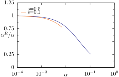
Figure 17: Renormalization factor $\alpha^{R}/\alpha$ of the dissipation strength from Eq. (63) computed for $\Delta/\omega_{c}=0.1$ as a function of $\alpha$ up to the critical point ($\alpha_{c}=0.007,0.105$ respectively for the two values $s=0.1,0.5$).

This quantity is plotted in Fig. 17 for two values of $s$ as a function of $\alpha<\alpha_{c}$, which shows that the full vertex $\Gamma$ remains finite up to the critical point, in agreement with our general expectation that this quantity remains regular at all orders in perturbation theory. Interestingly, the renormalization of the coupling constant $\alpha$ can be relatively large, up to 20% and 75% for the two cases $s=0.1$ and $s=0.5$ considered here. Such a sizeable effect will impact as well the fermionic self-energies, so that our consistent GW$\Gamma$ scheme will finally rely on the following set of equations:

$$\mathcal{I}m\Sigma_{x}^{GW\Gamma}(\omega) = \alpha^{R}\int_{0}^{\omega}\frac{\mathrm{d}\epsilon}{\pi}\mathcal{I}mG_{y}(\epsilon)\mathcal{I}mG_{\Phi}(\omega-\epsilon)$$ (64)

$$\mathcal{I}m\Sigma_{y}^{GW\Gamma}(\omega) = \alpha^{R}\int_{0}^{\omega}\frac{\mathrm{d}\epsilon}{\pi}\mathcal{I}mG_{x}(\epsilon)\mathcal{I}mG_{\Phi}(\omega-\epsilon)$$ (65)

$$\Sigma_{\Phi}^{GW\Gamma}(\omega) = \frac{\alpha^{R}}{2\Delta}$$ (66)

with $\alpha^{R}$ given in Eq. (63). The numerical implementation of the above equation, with self-consistency imposed by Dyson’s equations (26-29), is readily implemented, and gives the results displayed in Figs. 18 and 19 (we note again that fermionic self-consistency is only used in order to fill in the spurious gap of $C_{x}$, but it is not too important here).

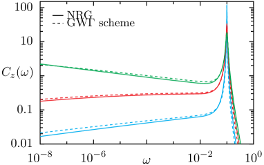
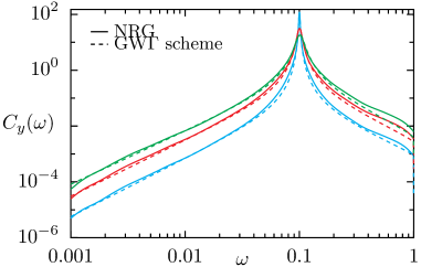
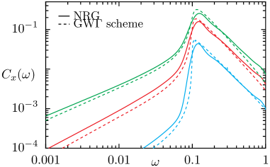
Figure 18: Spin susceptibilities $C_{z}(\omega)$, $C_{y}(\omega)$ and $C_{x}(\omega)$ (top to bottom panels) for $\Delta/\omega_{c}=0.1$, $s=0.1$ and increasing dissipation strength $\alpha=0.001,0.004,0.007$ (bottom to top), compared to the full Majorana diagrammatics (GW$\Gamma$ scheme).

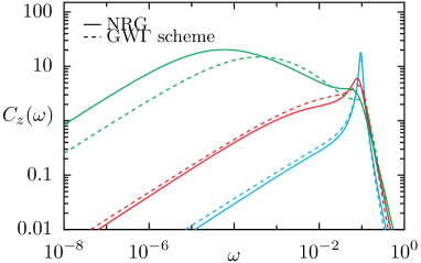
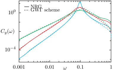
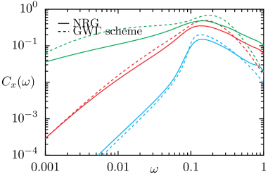
Figure 19: Spin susceptibilities $C_{z}(\omega)$, $C_{y}(\omega)$ and $C_{x}(\omega)$ (top to bottom panels) for $\Delta/\omega_{c}=0.1$, $s=0.5$ and increasing dissipation strength $\alpha=0.02,0.06,0.1$ (bottom to top), compared to the full Majorana diagrammatics (GW$\Gamma$ scheme).

In the case $s=0.1$, the outcome of the Majorana diagrammatics is at par with the NRG results for all three spin susceptibilities, both at low and high energies, and including the quantum critical regime. For the larger $s=0.5$ value, agreement is still quite good, and the visible deviations in the quantum critical regime (for $\alpha=0.1$) arise from slight discrepancies in the critical $\alpha_{c}$ between the diagrammatics and the NRG, so that the crossover scale is not accurately captured. We emphasize that this quantitative description of the spin dynamics relies of the weak coupling nature of the spin boson model for small $s$ values. The key step here was to understand that the most important contributions to the diagrammatics are the renormalization (beyond leading order) of the bosonic mass shift and the vertex corrections. It is possible that analytical renormalization group techniques (such as developed in Ref. Fritz, for the quantum phase transition in the pseudogap Kondo problem at weak coupling) may be applied to the spin-boson Hamiltonian based on the present understanding, but this would likely require more complex machinery to obtain similar results. This successful comparaison seals our study of the spin dynamics in delocalized phase of the spin-boson model.

V Conclusion

We have investigated the equilibrium spin dynamics of the sub-ohmic spin-boson model, which generically describes a two-level quantum system coupled to a dissipative environment of harmonic oscillators (characterized by a power-law spectrum $J(\omega)=2\pi\alpha\omega_{c}^{1-s}\omega^{s}\theta(\omega)\theta(\omega_{c}-\omega)$ with $s\leq 1$) and submitted to a perpendicular magnetic field $\Delta$. Two complementary techniques were employed, that were quantitatively benchmarked against each other. First, the bosonic Numerical Renormalization Group (NRG) was used with an optimized broadening method (“b-trick”) to obtain reliably the dynamical spin susceptibilities from weak ($\alpha\ll 1$) to strong ($\alpha\simeq 1$) dissipation. Here, we considered not only the usual transverse spin susceptibility (orthogonal to the field and parallel to the bosonic bath), but also for the first time the longitudinal (parallel to the field) and the second transverse (orthogonal to both bath and field) ones. Second, we established a general Majorana-fermion diagrammatic perturbation theory, controlled in the weak dissipation limit $\alpha\ll 1$. Because the spin-localization quantum phase transition takes place at a critical value $\alpha_{c}$ which becomes perturbatively accessible ($\alpha_{c}\ll 1$) either in the small field limit ($\Delta\ll\omega_{c}$ for all $s<1$) or in the strong sub-ohmic regime ($s\ll 1$ for all $\Delta/\omega_{c}$), it was possible to extend the diagrammatic method up to the quantum critical point. We then examined precisely how various flavors of GW-like approximations perform against the numerically exact results, in two different regimes. For $\alpha\ll\alpha_{c}$, bare perturbation theory (analogous to the standard Bloch-Redfield approximation for the non-equilibrium dynamics) was sufficient to describe well the finite energy dissipative features near the applied magnetic field $\Delta$, but fermionic self-consistency was needed in order to improve both on the low and high energy parts of the spectrum. Self-consistency was required because some of the bare self-energies can show spurious gaps that are in reality filled by multiparticle excitations. For $\alpha\lesssim\alpha_{c}$, huge deviations appeared in the low-energy limit between lowest order perturbation theory and the NRG data, due to the proximity to the quantum critical point. We showed that the effective interaction mediated by the bosonic field was the crucial ingredient to correctly describe the physics close to criticality, and that it should include vertex corrections (at the ladder level) in the bosonic and fermionic self-energies for quantitative agreement with the numerics. Such diagrammatic contributions are difficult to evaluate for higher dimensional field theories of coupled fermions and bosons Hertz ; Vignale and are rarely considered (see however Ref. Rech, ). A two-loop analysis allowed us also to obtain a simple equation for the critical line, that describes the NRG phase diagram very accurately in a wide range of parameters. We also presented a proof of Shiba’s relation generalized to the sub-ohmic case and the derivation of an effective bosonic action that may support the validity of the quantum-to-classical mapping.

We finally discuss possible outlooks for the methodology and the ideas developed here. First, the addition of a magnetic field component $\epsilon S^{z}$ parallel to the quantization axis may be considered with special interest LeHur . Indeed, understanding the magnetization process is the next step towards a good description of the localized phase of the spin-boson model, which was non considered in the present work, and which has led to recent debate. Vojta ; Kirchner ; Rieger ; Erratum ; Anders ; Feshke ; Zhang ; TongTrunc Second, further extensions of the model to multiple bosonic environments present very interesting physics in the ohmic case, Novais which remains to be investigated in greater generality. Third, an important consequence of our results is that the long time equilibrium dynamics is never accurately captured by lowest order perturbation theory in the coupling between the spin and the environment (unless dissipation is vanishingly small). This remark should have deep implications for the out-of-equilibrium long-time dynamics in dissipative models, which ought to be re-examined beyond the Bloch-Redfield regime. Extension of the Majorana diagrammatic method to two-times Keldysh Green’s function could be also considered in the context of sudden quenches in the spin boson model near the quantum critical point. Lastly, considering the spin-boson Hamiltonian as a toy model for quantum criticality, the quantitative understanding achieved here may be relevant for field theories of electrons coupled to bosons in higher dimensions.

Appendix A Shiba’s relations for the sub-ohmic spin-boson model

The goal of this appendix is to provide a simple derivation of Shiba’s relation Eq. (16) generalized to the sub-ohmic case. The first step of the proof is to note that the linear coupling between the $z$ component of the spin and the bosonic continuum, see Hamiltonian Eq. (1), implies an exact relation between the longitudinal spin susceptibility and the full retarded bosonic Green’s function:

$$G_{\Phi}(\omega)=G_{\Phi}^{0}(\omega)+\alpha[G_{\Phi}^{0}(\omega)]^{2}\chi_{z}(\omega)$$ (67)

where the bare bosonic Green’s function $G_{\Phi}^{0}(\omega)$ was introduced in the previous equation (30). This connection can be easily established from the use of equations of motions, or equivalently by using standard manipulation of a path-integral representation of the problem. The second step lies in a low-energy analysis of the bosonic propagator $G_{\Phi}(\omega)$ from the diagrammatic perspective. The key point is that the bosonic self-energy $\Sigma_{\Phi}(\omega)$, which was defined in Eq. (29) and expressed diagrammatically in Fig. 7, has a regular low-frequency behavior, owing to the role of the transverse magnetic field $\Delta$ in the bare Majorana Green’s function $G_{y}^{0}(\omega)$, see Eq. (23). As a consequence, all bosonic self-energy diagrams are cut in the long-time limit due to this energy gap, so that $\Sigma_{\Phi}(\omega)=\Sigma_{\Phi}(0)+\mathcal{O}(\omega)$ at low energy. Although the gap will be in reality filled by low energy excitations if one considers the full Majorana propagator $G_{y}(\omega)$, we have seen in Sec. III.2 that a quickly vanishing tail of excitations is obtained, so that the above argument persists non-perturbatively (provided that perturbation theory is convergent). As a concrete illustration, equation (51) computed at one-loop order demonstrates the regular character of the bosonic self-energy in the small frequency limit. Accounting for the static part of the self-energy within the explicit Dyson equation (LABEL:critical), and neglecting the term $\Sigma_{\Phi}(\omega)-\Sigma_{\Phi}(0)$ at low energy, one obtains:

$$G_{\Phi}(\omega)\simeq\frac{1}{m_{\Phi}}-\frac{ib}{(m_{\Phi})^{2}}\mathrm{Sign}(\omega)|\omega|^{s}$$ (68)

where the full mass $m_{\Phi}$ was given in Eq. (44). Similarly, the bare correlation function obeys a similar behavior:

$$G_{\Phi}^{0}(\omega)\simeq\frac{1}{m_{\Phi}^{0}}-\frac{ib}{(m_{\Phi}^{0})^{2}}\mathrm{Sign}(\omega)|\omega|^{s}$$ (69)

now involving the bare mass $m_{\Phi}^{0}$. We finally use the exact relation (67) in the low energy limit, which imposes two conditions by taking the real and imaginary parts:

$$\frac{1}{m_{\Phi}} = \frac{1}{m_{\Phi}^{0}}+\frac{\alpha}{(m_{\Phi}^{0})^{2}}\chi_{z}^{\prime}(0)$$ (70)

$$-\frac{b}{(m_{\Phi})^{2}}\mathrm{Sign}(\omega)|\omega|^{s} = -\frac{b}{(m_{\Phi}^{0})^{2}}\mathrm{Sign}(\omega)|\omega|^{s}+\alpha\frac{\chi_{z}^{\prime\prime}(\omega)}{(m_{\Phi}^{0})^{2}}$$ (71)

$$-\alpha\frac{2b}{(m_{\Phi}^{0})^{3}}\chi_{z}^{\prime}(0)\mathrm{Sign}(\omega)|\omega|^{s}$$

Solving this system to eliminate the mass $m_{\Phi}$ leads to the simple expression:

$$\chi_{z}^{\prime\prime}(\omega)\simeq\frac{-b}{(m_{\Phi}^{0})^{2}}\alpha|\omega|^{s}[\chi_{z}^{\prime}(0)]^{2}$$ (72)

asymptotically exact in the small $\omega$ limit. Using the known value for the coefficient $-b/(m_{\Phi}^{0})^{2}=2\pi\omega_{c}^{1-s}$ from Eq. (32), and relation (14), we finally obtain the generalized Shiba relation Eq. (16).

Appendix B Quantum-to-classical mapping

We can reformulate the usual quantum-to-classical mapping Emery in terms of an effective quantum action in imaginary time calculated perturbatively in the coupling constant $\alpha$. Indeed, in the $\epsilon\rightarrow 0$ limit, we first notice that the linear form of the coupling in the Hamiltonian Eq. (1) leads to the exact relation:

$$\big{<}S^{z}\big{>}=\frac{s}{4\sqrt{\alpha}\omega_{c}}\big{<}\Phi\big{>}$$ (73)

which can be derived by the same strategy as discussed in Appendix A. This result implies that the critical behavior of the impurity spin magnetization $\big{<}S^{z}\big{>}$ can be extracted from the knowledge of the bosonic static average. The static critical properties can thus be alternatively understood from the point of view of an effective action for the boson $\Phi$ only, which is obtained by integrating out the spin degrees of freedom perturbatively in $\alpha$. This can be done diagrammatically using the Majorana fermions, leading after some standard manipulations to the following expression in imaginary frequency:

$$S_{{\mathrm{eff}}}[\Phi]=\frac{1}{2}\int\frac{d\nu}{2\pi}\left(m_{\Phi}+A|\nu|^{s}\right)|\Phi(i\nu)|^{2}+\int d\tau\;u\;[\Phi(\tau)]^{4}$$ (74)

where $A\propto\omega_{c}^{-1-s}$. The first important parameter here is the bosonic mass $m_{\Phi}=s/(4\omega_{c})-\alpha/(2\Delta)+\mathcal{O}(\alpha^{2})$, which agrees with the one-loop result of Eq. (51), and controls the distance to the quantum critical point at leading order. The second crucial term is the $\Phi^{4}$ interaction with coefficient $u=\alpha^{2}/(16\Delta^{3})+\mathcal{O}(\alpha^{3})$.

Within the delocalized phase, i.e. as long as the renormalized mass $m_{\Phi}^{R}$ does not vanish, the bosonic spectral function obeys the low-frequency behavior $G_{\Phi}(i\nu)\propto 1/(m_{\Phi}^{R}+A|\nu|^{s})\propto 1/m_{\Phi}^{R}-A|\nu|^{s}/(m_{\Phi}^{R})^{2}$, i.e. the slow decay in imaginary time $G_{\phi}(\tau)\propto 1/\tau^{1+s}$. Owing to the exact relation (67), we recover the correct small frequency behavior of the longitudinal spin susceptibility, see Eq. (40). The low-energy sector of the spin-boson model is thus well captured by the effective bosonic action (74), which turns out to be equivalent to an Ising model in imaginary time with long-range spin exchange decaying as $1/(\tau-\tau^{\prime})^{1+s}$, exactly as expected from the quantum/classical equivalence Emery ; Bulla .

Let us finally discuss the low energy behavior at the quantum critical point. Scaling analysis relative to the massless theory ($m_{\Phi}=0$) leads to the bare scaling dimension $[u]=2s-1$. Thus, $u$ is relevant when $1/2<s$ and irrelevant otherwise. Therefore, in the weakly sub-ohmic regime $1/2<s<1$, the phase transition is described by an interacting fixed point Fisher and the magnetization $\big{<}S^{z}\big{>}$ obeys non-trivial classical exponents, as verified in the numerical study of Ref. Bulla, . On the contrary, in the strongly sub-ohmic range $0<s<1/2$, $u$ is irrelevant and mean-field theory should apply, a result that was recently debated. Vojta ; Kirchner ; Rieger ; Erratum ; Anders ; Feshke ; Zhang ; TongTrunc The effective action (74) would therefore tend to strengthen the idea that the quantum-to-classical mapping is robust, unless the Landau parameter $u$ picks up non-analyticities (such as discussed in Ref. BK1, ; BK2, for field theories involving coupled fermions and bosons in higher dimensions). However, the regularity of the diagrammatics would lead us to believe that this possibility is unlikely for the spin-boson model.

References

- (1) A. J. Leggett, S. Chakravarty, A. T. Dorsey, M. P. A. Fisher, A. Garg and W. Zwerger, Rev. Mod. Phys. 59, 1 (1987).
- (2) U. Weiss, Quantum Dissipative Systems, World Scientific, Singapore (1993).
- (3) M. Vojta, Phil. Mag. 86, 1807 (2006).
- (4) K. Le Hur in ”Understanding Quantum Phase Transitions” (Taylor and Francis, Boca Raton, 2010).
- (5) S. Florens, D. Venturelli, and R. Narayanan, Lect. Notes Phys. 802, 145 (2010), also in arXiv:1106.2654.
- (6) S. Sachdev, Quantum Phase Transitions, Cambridge University Press, Cambridge (1999).
- (7) D. G. Clarke, T. Giamarchi and B. I. Shraiman, Phys. Rev. B 48, 7070 (1993).
- (8) E. Novais, A. H. Castro Neto, L. Borda, I. Affleck and G. Zarand, Phys. Rev. B 72, 014417 (2005).
- (9) M. Vojta, C. Buragohain, and S. Sachdev, Phys. Rev. B 61, 15152 (2000).
- (10) A. I. Larkin and V. I. Mel’nikov, Sov. Phys. JETP 34, 656 (1972).
- (11) Y. L. Loh, V. Tripathi and M. Turlakov, Phys. Rev. B 71, 024429 (2005).
- (12) A. M. Sengupta and A. Georges, Phys. Rev. B 52, 10295 (1995).
- (13) A. M. Sengupta, Phys. Rev. B 61, 4041 (2000).
- (14) Q. Si and J. L. Smith, Phys. Rev. Lett. 77, 3391 (1996).
- (15) A. Georges, G. Kotliar, W. Krauth and M. Rozenberg, Rev. Mod. Phys. 68, 13 (1996).
- (16) A. C. Hewson, “The Kondo Problem to Heavy Fermions”, Cambridge University Press, Cambridge (1993).
- (17) S. Florens, A. Freyn, N. Roch, W. Wernsdorfer, F. Balestro, P. Roura-Bas, and A. A. Aligia, J. Phys.: Condens. Matter 23, 243202 (2011).
- (18) V. J. Emery and A. Luther, Phys. Rev. B 9, 215 (1974).
- (19) R. Bulla, N-H Tong and M. Vojta, Phys. Rev. Lett. 91, 170601 (2003).
- (20) M. E. Fisher, S. K. Ma and B. G. Nickel, Phys. Rev. Lett. 29, 917 (1972).
- (21) J. M. Kosterlitz, Phys. Rev. Lett. 37, 1577 (1976).
- (22) M. Vojta, N-H Tong and R. Bulla, Phys. Rev. Lett. 94, 070604 (2005).
- (23) S. Kirchner, Q. Si and K. Ingersent, Phys. Rev. Lett. 102, 166405 (2009).
- (24) A. Winter, H. Rieger, M. Vojta and R. Bulla, Phys. Rev. Lett. 102, 030601 (2009).
- (25) M. Vojta, N.-H. Tong, and R. Bulla, Phys. Rev. Lett. 102, 249904(E) (2009).
- (26) M. Vojta, R. Bulla, F. Güttge, and F. Anders, Phys. Rev. B 81, 075122 (2010).
- (27) A. Alvermann, and H. Fehske, Phys. Rev. Lett. 102, 150601 (2009).
- (28) Y.-Y. Zhang, Q.-H. Chen, and K.-L. Wang, Phys. Rev. B 81, 121105 (2010).
- (29) Y.-H. Hou, and N.-H. Tong, Euro. Phys. J. B 78, 127 (2010).
- (30) Z. Lü, and H. Zheng, Phys. Rev. B 75, 054302 (2007).
- (31) K. G. Wilson, Rev. Mod. Phys. 47, 773 (1975).
- (32) R. Bulla, T. Costi and T. Pruschke, Rev. Mod. Phys. 80, 395 (2008).
- (33) R. Bulla, H. J. Lee, N. H. Tong and M. Vojta, Phys. Rev. B 71, 045122 (2005).
- (34) W. Mao, P. Coleman, C. Hooley and D. Langreth, Phys. Rev. Lett. 91, 207203 (2003).
- (35) A. Shnirman and Y. Makhlin, Phys. Rev. Lett. 91, 207204 (2003).
- (36) M. Z. Hasan and C. L. Kane, Rev. Mod. Phys. 82, 3045 (2010).
- (37) A. Shnirman and G. Schoen, in “Quantum Noise in Mesoscopic Physics” (Delft, 2002), also arXiv:cond-mat/0210023.
- (38) P. Nalbach, and M. Thorwart, Phys. Rev. B 81, 054308 (2010).
- (39) R. S. Whitney, J. Phys. A: Math. Theor. 41, 175304 (2008).
- (40) F. Nesi, E. Paladino, M. Thorwart, M. Grifoni, Europhys. Lett. 80, 40005 (2007).
- (41) F. B. Anders, R. Bulla and M. Vojta, Phys. Rev. Lett. 98, 210402 (2007).
- (42) A. Freyn and S. Florens, Phys. Rev. B 79, 121102 (2009).
- (43) T. A. Costi and C. Kieffer, Phys. Rev. Lett. 76, 1683 (1996).
- (44) W. C. Oliveira and L. N. Oliveira, Phys. Rev. B 49, 11986 (1994).
- (45) A. Freyn, and S. Florens, Phys. Rev. Lett. 107, 017201 (2011).
- (46) R. Bulla, T. A. Costi, and D. Vollhardt, Phys. Rev. B64, 045103 (2001).
- (47) A. Weichselbaum and J. von Delft, Phys. Rev. Lett. 99, 076402 (2007)
- (48) R. Peters, T. Pruschke and F. B. Anders, Phys. Rev. B 74, 245114 (2006).
- (49) R. Zitko and T. Pruschke, Phys. Rev. B 79, 085106 (2009).
- (50) V. L. Campo and L. N. Oliveira, Phys. Rev. B 72, 104432 (2005).
- (51) A. Weichselbaum, F. Verstraete, U. Schollwöck, J. I. Cirac and J. von Delft, Phys. Rev. B 80, 165117 (2009).
- (52) A. Rosch, T. A. Costi, J. Paaske and P. Wölfle, Phys. Rev. B 68, 014430 (2003).
- (53) G. F. Giuliani and G. Vignale, Quantum Theory of the Electron Liquid Cambridge, 2005.
- (54) J. Hertz, Phys. Rev. B 14, 1165 (1976).
- (55) C. Di Castro, and R. Raimondi, in “The Electron Liquid Paradigm in Condensed Matter Physics”, (Varenna, 2003), also arXiv:cond-mat/0402203.
- (56) P. Nalbach, and M. Thorwart, J. Chem. Phys. 132, 194111 (2010).
- (57) L. Fritz, S. Florens, and M. Vojta, Phys. Rev. B 74, 144410 (2006).
- (58) J. Rech, C. Pépin, and A. V. Chubukov, Phys. Rev. B 74, 195126 (2006).
- (59) K. Le Hur, P. Doucet-Beaupré, and W. Hofstetter Phys. Rev. Lett. 99, 126801 (2007).
- (60) T. Vojta, D. Belitz, R. Narayanan, and T. R. Kirkpatrick, Europhys. Lett. 36, 191 (1996).
- (61) D. Belitz, T. R. Kirkpatrick, and T. Vojta, Rev. Mod. Phys. 77, 579 (2005).