Non-linear matter power spectrum from Time Renormalisation Group: efficient computation and comparison with one-loop

Abstract:

We address the issue of computing the non-linear matter power spectrum on mildly non-linear scales with efficient semi-analytic methods. We implemented M. Pietroni’s Time Renormalization Group (TRG) method and its Dynamical 1-Loop (D1L) limit in a numerical module for the new Boltzmann code CLASS. Our publicly released module is valid for $\Lambda$CDM models, and optimized in such a way to run in less than a minute for D1L, or in one hour (divided by number of nodes) for TRG. A careful comparison of the D1L, TRG and Standard 1-Loop approaches reveals that results depend crucially on the assumed initial bispectrum at high redshift. When starting from a common assumption, the three methods give roughly the same results, showing that the partial resumation of diagrams beyond one loop in the TRG method improves one-loop results by a negligible amount. A comparison with highly accurate simulations by M. Sato & T. Matsubara shows that all three methods tend to over-predict non-linear corrections by the same amount on small wavelengths. Percent precision is achieved until $k\sim 0.2\,h$Mpc^-1 for $z\geq 2$, or until $k\sim 0.14\,h$Mpc^-1 at $z=1$.

1 Motivations

Large scale structures in our universe have formed during the matter dominated era, starting from a very homogeneous state. In order to explain this mechanism, one must compute the evolution of the dominating species during this period: Cold Dark Matter (CDM) and baryons in the standard $\Lambda$CDM Model. It is generally agreed that structures formed from the gravitational collapse of small density perturbations. Depending on their wavelength, they entered at different times within the Hubble scale, which plays the role of a causal horizon for this process. Perturbations with very large wavelength, or very small wave number, had no time to evolve significantly beyond the linear regime. In practice, one can apply the linear perturbation theory for wave numbers smaller than $0.1h$Mpc^-1. In the opposite limit, for scales under $\sim 10$ Mpc today, the presence of highly non-linear structures such as galaxies points out the need for completely non-linear computations. This is taken care of by N-body simulations, that follow the evolution of a large ensemble of galaxies.

Current and upcoming surveys such as the Sloan Digital Sky Survey , the Large Synoptic Survey Telescope  and other Large Scale Structure (LSS) experiments probe this evolution with increasingly high precision. Through these new observations, cosmology opens a new window to confirm, constrain or infirm different high energy physics scenarios, related for instance to: neutrino masses, inflationary and dark energy models, or modifications of gravity.

The discriminating power of LSS observations depends crucially on the maximum wavenumber used in the comparison with the theory. By limiting the analysis to linear scales with $k<k_{max}=0.1h$Mpc^-1, one loses a lot of sensitivity, since the total amount of information scales like $k_{max}^{3}$. For instance, the strong dependence of neutrino mass error bars on $k_{max}$ is illustrated in [1]. To further enhance the sensitivity, one would be tempted to use highly detailed N-body simulations. Unfortunately, in order to find both the best-fitting values and the error bars of the free cosmological parameters of a given scenario, one needs to compute a huge number of theoretical spectra corresponding to different points in parameter space. With the most efficient techniques (Monte Carlo Markov Chains), a minimum of 10’000 to 100’000 points is necessary, depending on the complexity of the model. N-body simulations are far too slow for being carried in each of these points, or even in sizable fraction of them. This raises the need for semi-analytical tools to make accurate predictions on interesting scales. Even if such tools remain accurate only in a small range of mildly non-linear scales (just above $0.1h$Mpc^-1), they can play a crucial role in measuring quantities like neutrino masses.

Some of these semi-analytical tools just consist in fitting formulas calibrated to N-body simulation, as for instance HALOFIT [2]. HALOFIT represents the fastest thinkable way to account for non-linear perturbations, but its range of validity is limited to the minimal $\Lambda$CDM model. Extending it to non-minimal cosmological scenarios requires many N-body simulations (and in some cases, like for models containing species with a sizable free-streaming length, carrying any N-body simulation remains very involved). Moreover, HALOFIT does not provide a good fit to the Baryon Acoustic Oscillations (BAOs) in the non-linear spectrum.

Other semi-analytical methods have been proposed to actually calculate the non-linear power spectrum in Fourier space, taking into account the effects of mode coupling to some extent (for reviews and comparisons, see e.g. [3, 4, 5, 6, 7, 8]). Of course, all these approaches fail when dealing with the highly non-linear regime. However, their formulation stays consistent within the mildly non-linear regime, up to some $k_{max}$ which depends on the method. Any tool implementing a good compromise between computing time on the one hand, and accuracy (i.e. large $k_{max}$) on the other hand, can be extremely useful for two purposes: first, for calibrating fitting formulas in the mildly non-linear regime for extended cosmological scenarios, without running N-body simulations; second, if the method is fast enough, for being employed at each point in parameter space when fitting cosmological models to the data.

In this paper, we concentrate on the Time Renormalization Group (TRG) method proposed by Massimo Pietroni [6]. This method consists in integrating over time a coupled system of differential equations for the density and velocity power spectra and bispectra. Since the non-linearity computed at a given time step affect the time-derivative of the spectra at this step, the TRG method continuously includes higher-order corrections to the linear power spectra, and can be seen as a simple way to resum a sub-class of diagrams beyond one loop.

A simple variant of the TRG equations, consisting in using products of the linear power spectra in the non-linear source term of the equations, provides strictly one-loop results. However, the one-loop power spectrum computed in that way is obtained from dynamical equations (we actually call this method D1L for Dynamical 1-Loop). This should be contrasted with the Standard 1-Loop (S1L) method in which the time evolution is integrated away, using some simplifying assumptions. The main focus of this paper consists in a detailed comparison between S1L, D1L and TRG results for realistic $\Lambda$CDM models. We will see that assumptions concerning the initial bispectrum at high redshift crucially affect the results al low redshift. This point had been overlooked in the past, and will lead us to the conclusion that when starting from the same assumptions, the three methods only differ by a negligible amount. Hence, using the TRG method (at the order discussed in the current literature) instead of the much faster D1L algorithm does not appear to be justified.

We also provide some details about our numerical implementation of these methods in the form of a C module for the new Boltzmann code CLASS [9, 10], released with the version v1.2 of the code. Our implementation allows for a small computing time (for the TRG method, 70 minutes on a single-core CPU, to be divided by the number of cores in a parallel execution; and for D1L, less than a minute), opening the possibility to integrate it within a parameter extraction code. These approaches could easily be used e.g. for computing CMB lensing or cosmic shear power spectra in the mildly non-linear regime, without recurring to any N-body simulation or empirical fitting formulas. They also provide the non-linear velocity and cross density-velocity power spectra.

We review the standard one-loop approach very briefly in section 2, M. Pietroni’s TRG method in section 3, and our numerical implementation of the previous equations in section 4. We present some self-consistency checks in the exact Einstein-De-Sitter (EdS) limit in 5, and show our results for a realistic $\Lambda$CDM model in section 6. We include a comparison with N-body simulations performed with GADGET [11] by Sato & Matsubara [8], and with HALOFIT. A summary is provided in section 7. Appendix A recalls how the continuity and Euler equations are derived from the Boltzmann equation. Finally, Appendix B provides details on the code itself.

2 Standard one-loop approach

The one-loop density power spectrum is usually computed at any redshift using the formula

$$P_{\mathrm{NL}}(k)=P_{\mathrm{L}}(k)$$ (1)

$$+\frac{2\pi}{k}\int_{0}^{\infty}dpP_{\mathrm{L}}(p)\left\{\int_{|p-\frac{k}{2}|+\frac{k}{2}}^{k+p}dqP_{\mathrm{L}}(q)\left(\frac{\left(2k^{4}+3k^{2}(q^{2}+p^{2})+10p^{2}q^{2}-5(p^{4}+q^{4})\right)^{2}}{14^{2}p^{3}q^{3}}\right)\right.$$

$$+\left.\frac{k^{3}P_{\mathrm{L}}(k)}{252}\left(\frac{12k^{2}}{p^{2}}-158+\frac{100p^{2}}{k^{2}}-\frac{42p^{4}}{k^{4}}-\frac{3k^{3}}{p^{3}}\left(\frac{7p^{2}}{k^{2}}+2\right)\left(\frac{p^{2}}{k^{2}}-1\right)^{3}\ln\frac{\left|1-\frac{p}{k}\right|}{1+\frac{p}{k}}\right)\right\}~{},$$

where $P_{\mathrm{L}}(k)$ is the linear density power spectrum (see e.g. [3] and references therein). This result, that we will call S1L for Standard 1-Loop, is obtained by expanding the density and velocity fields describing a single-flow pressureless fluid at order two in perturbations. It is based however on additional approximations concerning the time-evolution of linear and non-linear perturbations.

Indeed, the above formula corresponds to the exact one-loop solution of the continuity and Euler equations for such a fluid only in the perfect Einstein-De-Sitter limit (more precisely, assuming that all modes obey to a newtonian evolution in a fully matter-dominated universe). In this case, the matter density perturbations can be expanded as

$$\delta(\tau,k)=\sum_{i=1}^{\infty}a(\tau)^{i}\delta^{(i)}(k)$$ (2)

where $\tau$ stands for conformal time, $a^{i}$ for the scale factor to the power $i$, and $\delta^{(i)}$ for the $i$-th order perturbation rescaled by $a^{i}$. A similar expansion is performed for the velocity divergence field $\theta$:

$$\theta(\tau,k)={\cal H}(\tau)\sum_{i=1}^{\infty}a(\tau)^{i}\theta^{(i)}(k)~{},$$ (3)

with ${\cal H}\equiv a^{\prime}/a$. When writing the relations between the $\delta^{(i)}$ and $\theta^{(i)}$ functions, all time-dependent factors simplify, thanks to the structure of the non-linear continuity and Euler equations. After collecting all terms, one can write the non-linear power spectrum as a function of the linear one evaluated at the same redshift, without any integral over time.

In a realistic $\Lambda$CDM universe, the linear density fluctuations undergo a complicated evolution at high redshift: their behavior is radically different on super/sub-Hubble scales, during radiation/matter domination, before/after photon decoupling. After recombination, when radiation perturbations become negligible, their evolution can be caught by a scale-independent growth factor often parametrized as $a(\tau)\times g(\tau)$, where $g$ is a function of time falling below one close to $\Lambda$ or Dark Energy domination. Similarly, the linear velocity divergence $\theta$ scales like $a(\tau)\times f(\tau)$, with $f\equiv g+a\,g^{\prime}/a^{\prime}$. We show $g(z)$ and $f(z)$ for typical $\Lambda$CDM parameters in figure 1.

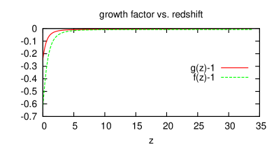
Figure 1: Functions $g(z)$ and $f(z)$ related to the linear growth factor of density perturbations and velocity divergence, for a $\Lambda$CDM model with $\Omega_{\Lambda}=0.735$.

As long as one can neglect massive neutrinos or eventual dark energy perturbations, high-order terms in perturbation theory should still be separable functions of time and wavenumber, because the model contains no characteristic length that could lead to a scale-dependent growth factor within the Hubble radius. However, these terms do not scale like powers of $[a\,g]$. This can be checked by trying an expansion of the type

$$\delta(\tau,k)=\sum_{i=1}^{\infty}[a(\tau)g(\tau)]^{i}\delta^{(i)}(k)~{},\qquad\theta(\tau,k)={\cal H}(\tau)\sum_{i=1}^{\infty}[a(\tau)g(\tau)]^{i}\theta^{(i)}(k).$$ (4)

Since the non-linear equations of motion still contain factors in $a^{\prime}/a$, not $[ag]^{\prime}/[ag]$, the time-dependence cannot be factored out in the same way as in the Einstein-De-Sitter case (for more details see e.g. [3, 6]). In summary, the formula (1) is only approximate, due to the non-trivial evolution of perturbation in a realistic $\Lambda$CDM universe, both at high redshift (recombination time and before) and at low redshift ($\Lambda$ domination).

In order to evaluate the corresponding error, one should compare the power spectrum obtained from eq. (1) with that obtained from a full integration over time of one-loop equations. This task becomes easy once the TRG equations have been correctly implemented, since the TRG method relies on dynamical equations, and since the one-loop order corresponds to a simple limit of these equations. A test presented in [6] suggests that the error induced by low-redshift effects is very small. Below, we will confirm this finding, but interestingly, we will show that the error induced by mistreating the initial bispectrum at high redshift is instead very significant.

3 Time Renormalization Group equations

For the rest of this article, the following conventions are assumed. The universe is considered to be described by the $\Lambda$CDM model, with zero spatial curvature. We assume Gaussian initial conditions, and therefore a vanishing bispectrum at initial time.

During the matter dominated era and within the Hubble radius, the matter velocity dispersion is small. It is therefore possible to use the Newtonian limit of the Einstein’s field equations for the perturbation of the energy tensor. By starting TRG computations at a redshift $z_{ini}=35$, and dealing only with non-linear equations for wavenumbers above $2.10^{-3}~{}h/Mpc$, one stays in the range where these approximations are valid.

In the TRG approach and within the $\Lambda$CDM paradigm, one has to renormalize both baryon and CDM. This could lead to a tedious system with mixed variables, since a priori baryons have non-negligible pressure (sound speed). However, pressure effects appears at very small scales (in any case, above $10~{}h/\text{Mpc}$), and it is safe to approximate baryons as pressureless and collisionless. Then, both baryon and CDM follow the same non-linear equations, and share the same initial condition provided that the starting redshift is chosen sufficiently far from decoupling (which is the case with $z_{ini}=35$). They can be described as a single perturbation field, hereafter denoted as the matter field with subscript $m$, and all quantities $X_{m}$ are defined as $\Omega_{m}X_{m}=\Omega_{b}X_{b}+\Omega_{c}X_{c}$.

The non-linear collisionless Boltzmann equation of a self-gravitating fluid is the master equation describing structure formation, and being solved in N-body simulations. In Appendix A, we recall the basic steps and assumptions allowing to reduce the Boltzmann equation to a coupled system of non-linear equations in Fourier space: namely, the continuity and Euler equation for density perturbations $\delta_{m}(\mathbf{k},\tau)$ and velocity divergence $\theta_{m}(\mathbf{k},\tau)$.

In order to solve these equations, the most common approach consists in expanding $\delta_{m}$ and $\theta_{m}$ in perturbations, and solve the system at a given order. The TRG relies on a different expansion, in connected $n$-point correlation functions. The two approaches start however from the same equations. One needs to introduce simplified notations similar to those in [4], and to define a doublet $\varphi_{a}$ (a=1,2):

$$\begin{pmatrix}\varphi_{1}(\mathbf{k},\eta)\\ \varphi_{2}(\mathbf{k},\eta)\end{pmatrix}\equiv e^{-\eta}\begin{pmatrix}\delta_{m}(\mathbf{k},\eta)\\ -\theta_{m}(\mathbf{k},\eta)/\mathcal{H}\end{pmatrix}~{},$$ (5)

where $\eta=\log(a/a_{\text{ini}})$. The role of the exponential term consists in factorizing out most of the time evolution. Indeed, the variables $\varphi_{i}(\mathbf{k},\eta)$ are constant during matter domination and in the linear regime; their subsequent slow variation is easier to catch numerically than the fast variation of $(\delta_{m},\theta_{m})$. The non-linear continuity and Euler equations (eqs. (39,40) of Appendix A) can then be cast in a compact form:

$$\partial_{\eta}\varphi_{a}(\mathbf{k},\eta)=-\Omega_{ab}(\mathbf{k},\eta)\varphi_{b}(\mathbf{k},\eta)+e^{\eta}\gamma_{abc}(\mathbf{k},-\mathbf{p},-\mathbf{q})\varphi_{b}(\mathbf{p},\eta)\varphi_{c}(\mathbf{q},\eta),$$ (6)

where we follow the Einstein convention for repeated indices (sum) and momentum (integral on $\mathbf{p}$ and $\mathbf{q}$). The vertex functions $\gamma_{abc}(\mathbf{k},\mathbf{p},\mathbf{q})$ (a,b,c=1,2), encoding the non-linearity, are defined through:

$$\gamma_{121}(\mathbf{k},\mathbf{p},\mathbf{q}) =\frac{1}{2}\delta_{D}(\mathbf{k}+\mathbf{p}+\mathbf{q})\alpha(\mathbf{p},\mathbf{q}),$$ (7)

$$\gamma_{222}(\mathbf{k},\mathbf{p},\mathbf{q}) =\delta_{D}(\mathbf{k}+\mathbf{p}+\mathbf{q})\beta(\mathbf{p},\mathbf{q}),$$ (8)

$$\gamma_{112}(\mathbf{k},\mathbf{p},\mathbf{q}) =\gamma_{121}(\mathbf{k},\mathbf{q},\mathbf{p}),$$ (9)

and all other components vanish. The definition of the kernels $\alpha$ and $\beta$ is given in eqs. (41) of Appendix A. The $\Omega$ matrix, accounting for the linear evolution, reads

$$\begin{pmatrix}1&-1\\ -\frac{3}{2}\Omega_{m}(\eta)(1+\mathcal{B}(\mathbf{k},\eta))&2+\frac{\mathcal{H}(\tau)^{\prime}}{\mathcal{H}(\tau)}\end{pmatrix},$$ (10)

including a factor $\mathcal{B}(\mathbf{k},\eta)=\sum_{i\neq m}\frac{\Omega_{i}\delta_{i}}{\Omega_{m}\delta_{m}}$ (in $\Lambda$CDM, $i$ runs only on photon and neutrino species) which appeared thought the Poisson equation. Although we are interested in following the matter perturbations non-linearly, we do not want to abandon altogether other species which might play an important role at the percent precision. The equations presented in this section include this effect, while those solved by the code do not. This issue will be discussed in more details in sections 4 and 7. A nice property of this formulation is that everything one would like to test about new cosmologies is entirely encoded in the $\Omega$ matrix, while the non-linear vertices are model-independent.

The equations of evolution for correlation functions of $\varphi_{a}$ can be derived by applying several times equation (6), omitting arguments for clarity:

$$\partial_{\eta}<\varphi_{a}\varphi_{b}> = -\Omega_{ac}<\varphi_{c}\varphi_{b}>-\Omega_{bc}<\varphi_{a}\varphi_{c}>$$

$$+e^{\eta}\gamma_{acd}<\varphi_{c}\varphi_{d}\varphi_{b}>+e^{\eta}\gamma_{bcd}<\varphi_{a}\varphi_{c}\varphi_{d}>,$$ (11)

$$\partial_{\eta}<\varphi_{a}\varphi_{b}\varphi_{c}> = -\Omega_{ad}<\varphi_{d}\varphi_{b}\varphi_{c}>-\Omega_{bd}<\varphi_{a}\varphi_{d}\varphi_{c}>-\Omega_{cd}<\varphi_{a}\varphi_{b}\varphi_{d}>$$

$$+e^{\eta}\gamma_{ade}<\varphi_{d}\varphi_{e}\varphi_{b}\varphi_{c}>+e^{\eta}\gamma_{bde}<\varphi_{a}\varphi_{d}\varphi_{e}\varphi_{c}>$$

$$+e^{\eta}\gamma_{cde}<\varphi_{a}\varphi_{b}\varphi_{d}\varphi_{e}>,$$ (12)

$$\partial_{\eta}<\varphi_{a}\varphi_{b}\varphi_{c}\varphi_{d}> = \dots$$

The power spectrum $P_{ab}$, bispectrum $B_{abc}$ and trispectrum $Q_{abcd}$ of the doublet components are defined as:

$$<\varphi_{a}(\mathbf{k},\eta)\varphi_{b}(\mathbf{q},\eta)>~{}\equiv~{}\delta_{D}(\mathbf{k}+\mathbf{q})P_{ab}(\mathbf{k},\eta)$$

$$<\varphi_{a}(\mathbf{k},\eta)\varphi_{b}(\mathbf{q},\eta)\varphi_{c}(\mathbf{p},\eta)>~{}\equiv~{}\delta_{D}(\mathbf{k}+\mathbf{q}+\mathbf{p})B_{abc}(\mathbf{k},\mathbf{q},\mathbf{p};\eta)$$

$$<\varphi_{a}(\mathbf{k},\eta)\varphi_{b}(\mathbf{q},\eta)\varphi_{c}(\mathbf{p},\eta)\varphi_{d}(\mathbf{j},\eta)>~{}\equiv$$

$$\hskip 56.9055pt\left[\delta_{D}(\mathbf{k}+\mathbf{q})\delta_{D}(\mathbf{p}+\mathbf{j})P_{ab}(\mathbf{k},\eta)P_{cd}(\mathbf{p},\eta)\right.$$

$$\hskip 56.9055pt+\delta_{D}(\mathbf{k}+\mathbf{p})\delta_{D}(\mathbf{q}+\mathbf{j})P_{ac}(\mathbf{k},\eta)P_{bd}(\mathbf{q},\eta)$$

$$\hskip 56.9055pt+\delta_{D}(\mathbf{k}+\mathbf{j})\delta_{D}(\mathbf{q}+\mathbf{p})P_{ad}(\mathbf{k},\eta)P_{bc}(\mathbf{q},\eta)$$

$$\hskip 56.9055pt\left.+\delta_{D}(\mathbf{k}+\mathbf{p}+\mathbf{q}+\mathbf{j})Q_{abcd}(\mathbf{k},\mathbf{q},\mathbf{p},\mathbf{j};\eta)\right]$$ (13)

One has to note that $P_{ab}$ will differ from the usual matter/velocity power spectrum by a factor $e^{2\eta}$ and some factors of $\mathcal{H}(\tau)$ in the case of $P_{\delta\theta}$ and $P_{\theta\theta}$. To close this system of equations, the approximation proposed by M. Pietroni consists in setting $Q_{abcd}$ to zero. Hence, the TRG does not consist in truncating at a given order in perturbations or loops, but at a given order in connected correlation functions. Assuming $Q_{abcd}=0$ should be valid up to some time in the non-linear evolution. This truncation still allows for a departure from gaussianity (the bispectrum is not set to zero at any time), and for evolving models with a non-zero primordial bispectrum. By putting together (13) and (11, 12), one finds a closed system of equations, corresponding to the TRG equations truncated at the trispectrum order:

$$\partial_{\eta}P_{ab}(\mathbf{k},\eta)= -\Omega_{ac}(\mathbf{k},\eta)P_{cb}(\mathbf{k},\eta)-\Omega_{bc}(\mathbf{k},\eta)P_{ac}(\mathbf{k},\eta)$$

$$+e^{\eta}\int\text{d}^{3}\mathbf{q}\left[\gamma_{acd}(\mathbf{k},-\mathbf{q},\mathbf{q}-\mathbf{k})B_{bcd}(\mathbf{k},-\mathbf{q},\mathbf{q}-\mathbf{k};\eta)\right.$$

$$\hskip 56.9055pt\left.+B_{acd}(\mathbf{k},-\mathbf{q},\mathbf{q}-\mathbf{k};\eta)\gamma_{bcd}(\mathbf{k},-\mathbf{q},\mathbf{q}-\mathbf{k},\eta)\right],$$ (14)

$$\partial_{\eta}B_{abc}(\mathbf{k},-\mathbf{q},\mathbf{q}-\mathbf{k};\eta)= -\Omega_{ad}(\mathbf{k},\eta)B_{dbc}(\mathbf{k},-\mathbf{q},\mathbf{q}-\mathbf{k};\eta)$$

$$-\Omega_{bd}(-\mathbf{q},\eta)B_{adc}(\mathbf{k},-\mathbf{q},\mathbf{q}-\mathbf{k};\eta)$$

$$-\Omega_{cd}(\mathbf{q}-\mathbf{k},\eta)B_{abd}(\mathbf{k},-\mathbf{q},\mathbf{q}-\mathbf{k};\eta)$$

$$+2e^{\eta}\left[\gamma_{ade}(\mathbf{k},-\mathbf{q},\mathbf{q}-\mathbf{k})P_{db}(\mathbf{q},\eta)P_{ec}(\mathbf{k}-\mathbf{q},\eta)\right.$$

$$\hskip 36.98866pt\gamma_{bde}(-\mathbf{q},\mathbf{q}-\mathbf{k},\mathbf{k})P_{dc}(\mathbf{k}-\mathbf{q},\eta)P_{ea}(\mathbf{k},\eta)$$

$$\hskip 34.14322pt\left.\gamma_{cde}(\mathbf{q}-\mathbf{k},\mathbf{k},-\mathbf{q})P_{da}(\mathbf{k},\eta)P_{eb}(\mathbf{q},\eta)\right].$$ (15)

These definitions are in agreement with the Fourier transform conventions adopted in this paper, namely, $A(\mathbf{k},\tau)=(2\pi)^{-3}\int\text{d}^{3}\mathbf{x}\exp(-i\mathbf{k}\mathbf{x})A(\mathbf{x},\tau)$. The other common definition, actually used in CLASS, reads $A(\mathbf{k},\tau)=\int\text{d}^{3}\mathbf{x}\exp(-i\mathbf{k}\mathbf{x})A(\mathbf{x},\tau)$. In this case, in the RHS of eq. (15), the last term picks up one extra $(2\pi)^{3}$ factor.

4 Numerical implementation

4.1 Integrated form of the equations

Our module does not rely on the full TRG equations, but on their integrated form already introduced in the original TRG paper [6], that we briefly summarize below.

As a consequence of the statistical homogeneity and isotropy of the universe, the power spectrum $P$ only depends on $k=|\mathbf{k}|$, while the $\gamma$ and $B$ functions that appear in (14) under the summation sign only depend of $|\mathbf{q}|$,$|\mathbf{k}-\mathbf{q}|$ and the angle between $\mathbf{k}$ and $\mathbf{q}$. Let us introduce a spherical coordinate system $(r,\theta,\varphi)$ such that $\mathbf{k}=(k,0,0)$ and $\mathbf{q}=(q,\theta,\varphi)$. When integrating over $\text{d}^{3}\mathbf{q}$, the integral over $\varphi$ yields a $2\pi$ factor. Then by performing the variable change between $\theta$ and $p$ defined as $p^{2}=|k+q|^{2}$, one can transform the measure to:

$$\int\text{d}^{3}\mathbf{q}=\frac{2\pi}{k}\int_{0}^{\infty}q\text{d}q\int_{|q-k|}^{q+k}p\text{d}p.$$ (16)

Finally, by analyzing the shape of the integration domain, it is possible to further simplify the integrand in (14) and get

$$\partial_{\eta}P_{ab}(k,\eta)= -\Omega_{ac}(k,\eta)P_{cb}(k,\eta)-\Omega_{bc}(k,\eta)P_{ac}(k,\eta)$$

$$+e^{\eta}\frac{4\pi}{k}\int_{k/2}^{\infty}q\text{d}q\int_{|q-k|}^{q}p\text{d}p\left[\gamma_{acd}(k,q,p)B_{bcd}(k,q,p;\eta)\right.$$

$$\hskip 56.9055pt\left.+B_{acd}(k,q,p;\eta)\gamma_{bcd}(k,q,p)\right],$$ (17)

where $\gamma_{abc}(k,q,p)\equiv\gamma_{abc}(\mathbf{k},\mathbf{q},\mathbf{p})|_{\mathbf{p}=-(\mathbf{k}+\mathbf{q})}$. In a numerical implementation, the bispectrum, being a function of three variables and three indices, is a large object. To reduce the dimensionality of the problem, it was already noticed by M. Pietroni that as long as the scale-dependence of the $\Omega$ matrix can be neglected, we can obtain a closed system in which the integrated quantities replacing the bispectrum read

$$I_{acd,bef}(k) \equiv\int_{k/2}^{\infty}q\text{d}q\int_{|q-k|}^{q}p\text{d}p\frac{1}{2}\left[\gamma_{acd}(k,q,p)B_{efg}(k,q,p)+(q\leftrightarrow p)\right].$$ (18)

According to eq. (15), the time evolution of $I$ is given by

$$\partial_{\eta}I_{acd,bef}(k)=-\Omega_{bg}I_{acd,gef}(k)-\Omega_{eg}I_{acd,bgf}(k)-\Omega_{fg}I_{acd,beg}(k)+2e^{\eta}A_{acd,bef}(k),$$ (19)

with the $A$’s being given by

$$A_{acd,bef}(k)\equiv\int_{k/2}^{\infty}dq~{}q\int_{|q-k|}^{q}dp~{}p\frac{1}{2}\left\{\gamma_{acd}(k,q,p)\left[\gamma_{bgh}(k,q,p)P_{ge}(q)P_{hf}(p)+\right.\right.$$

$$\left.\left.\gamma_{egh}(q,p,k)P_{gf}(p)P_{hb}(k)+\gamma_{fgh}(p,k,q)P_{gb}(k)P_{he}(q)\right]+(q\leftrightarrow p)\right\}.$$ (20)

In eq. (17), all integrals have been absorbed in the definition of $I$:

$$\partial_{\eta}P_{ab}(k) =-\Omega_{ac}P_{cb}(k)-\Omega_{bc}P_{ac}(k)+e^{\eta}\frac{4\pi}{k}[I_{acd,bcd}(k)+I_{bcd,acd}(k)].$$ (21)

Finally, we can perform a rotation from the $(q,p)$ basis into a new $(x,y)$ basis in order to obtain separable integration ranges:

$$\int_{k/2}^{\infty}dq~{}q \int_{|q-k|}^{q}dp~{}p\left[F(k,q,p)+(q\leftrightarrow p)\right]$$

$$=\int_{k/\sqrt{2}}^{\infty}\text{d}x\int_{0}^{k/\sqrt{2}}\text{d}y\frac{x^{2}-y^{2}}{2}\left[F(k,\frac{x+y}{\sqrt{2}},\frac{x-y}{\sqrt{2}})+(y\leftrightarrow-y)\right],$$ (22)

where $F$ is a generic notation for the integrands appearing in eq. (20).

We implemented this integrated approach in our module as a first step (which is already far from trivial from the numerical point of view). Having checked this level of approximation, we aim to go back to the full set of equations in the future. This would allow to compute the full bispectrum evolution, starting from Gaussian or non-Gaussian initial conditions. It would also allow to treat consistently the case of a matrix $\Omega$ with a significant scale-dependence, and to perform a more robust test of the approximation used in [12, 13, 14], in which the above method was employed in the presence of massive neutrinos or dark energy perturbations.

By analyzing the symmetries of eq. (20), (18) and (7), (8), one can reduce the number of independent $I_{acd,bef}(k)$ functions from $64$ to $14$: namely, the set $(121,def)$ with $(def)=(111),(211),(121),(112),(122),(212),(221),(222)$ and the set $(222,ghi)$ with $(ghi)=(111),$$(211),$$(121),$$(122),$$(212),$$(222)$. Hence, we must solve a system of 17 differential equations (3 for $P_{ab}$ and 14 for $I_{acd,bef}$). The only time-consuming step is the evaluation of the 14 two-dimensional integrals of eq. (20) at each time step.

4.2 The three modes

Our numerical module can be tuned in such a way to solve either the above equations, or some limit of these equations, in order to reproduce different approaches.

4.2.1 Linear mode

First, by setting all the $A$ coefficients to zero, we can integrate the linear part of equations (19, 21) and try to reproduce the linear evolution of the power spectrum between $z_{ini}$ and today. Comparing these results with very accurate ones produced directly by the Boltzmann code is actually a useful way to estimate the precision of the time integration algorithm inside the TRG module, as we shall see in section 4.3. This calculation is performed when the CLASS input parameter “non linear” is set to “test-linear”.

4.2.2 TRG mode

The full solution of the TRG equations, computed when the CLASS input parameter “non linear” is set to “trg”, is of course much more time-consuming, since $14$ independent $A$ terms must be computed at each time step. The code has been parallelized with OpenMP. Its running time is of the order of 70 minutes on a single 2.3GHz core for the set of default accuracy parameters described in the next subsections and in Appendix B, and on a multi-core machine the running time scales almost linearly (i.e. 5 minutes on 14 cores, which is an optimal choice due to the structure of the equations).

4.2.3 Dynamical 1-Loop (D1L) mode

Next, by computing the integrals of eq. (20) using the linear power spectra at each time, one expects to reproduce standard results from one-loop perturbation theory. In this paper, we will call this method D1L for Dynamical 1-Loop. As explained in [6], in an Einstein-De-Sitter universe, the D1L equations can be integrated over time analytically, and then reduced to eq. (1). In realistic cosmological models, the linear spectra $P_{ab}$ are time dependent, and the 14 $A$ terms need to be evaluated at each time, leading to an algorithm essentially as time-consuming as the full TRG one. However, as long as we stick to $\Lambda$CDM models, we can use the fact that the linear spectra evolution is accounted by scale-independent growth factors, in such a way that $P_{11}^{\rm linear}(k,\eta)\propto g^{2}(\eta)$, $P_{22}^{\rm linear}\propto f^{2}$, and $P_{12}^{\rm linear}\propto gf$. So, the time dependence of the integrals of eq. (20) computed with the linear spectra factors out, leading to a very fast algorithm.

In practise, before starting the computation, we get $g(\eta)$ and $f(\eta)$ at each time-step using other CLASS modules. We compute the integrals of eq. (20) at initial time $\eta_{\rm ini}$. Then, at each new time step, we source the TRG equations with the same integrals rescaled by the appropriate number of factors $(g/g_{\rm ini})$ and $(f/f_{\rm ini})$. This calculation is performed in the publicly released module when the CLASS input parameter “non linear” is set to “one-loop”. It provides one-loop results for $\Lambda$CDM models with no approximation regarding the time evolution of perturbations, while being nearly as fast as the S1L method. We will see in section 6 that it greatly improves over S1L predictions.

4.3 Time integration

The time integration is performed with a predictor-corrector method. Starting from a time $\eta$ at which all quantities are known, one computes the new $P$ and $I$ functions at the step $\eta+\delta\eta/2$ with the standard Euler method, as well as their derivatives in this point. The values of $P$ and $I$ at $\eta+\delta\eta$ are then derived with the Euler method, using however the derivatives at the mid-point. With respect to a basic Euler method, this allows to take many less steps for the same level of accuracy (typically, we use between $50$ and $100$ time steps to evolve from $z=35$ to the present time).

With a predictor-corrector method on $100$ time steps, and at all redshifts and wave-numbers of interest, we find that the linear spectrum calculated by the TRG module agrees at the $0.05\%$ level with the one calculated by CLASS (with many more time steps and a sophisticated integrator). With $50$ time steps, the error is still as low as $0.08\%$, allowing us to keep this choice as a default setting in the released version of the code. The convergence has also been controlled for the one-loop computation: with only $50$ steps and a predictor-corrector method, one reaches the same $0.1\%$ level accuracy as with $10^{\prime}000$ steps and a standard Euler method.

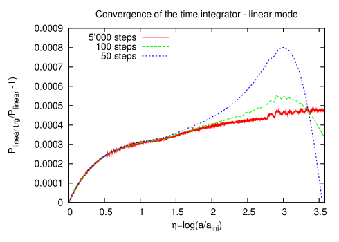
Figure 2: Convergence proof of the linear time-evolution in the TRG module w.r.t. the linear evolution in CLASS.

4.4 Momentum integration

Since in the TRG module, most of the time is spent in the computation of $A$ functions, an obvious way to speed up the code would be to make a cut in the domain of integration. This domain, defined in eq. (22), has a rectangular shape ($x>k/\sqrt{2}$, $0<y<k/\sqrt{2}$).

After noticing that the main contribution to the integral comes from the region near the $x=k/\sqrt{2}$ and $y=k/\sqrt{2}$ boundaries, and that the integrand exhibits an approximate symmetry around the axis $y=\sqrt{2}k-x$, we first tried to integrate on L-shaped bands starting from the top left corner in $(x,y)$ space. One could hope that after integrating over a few such L’s, the integration would converge and could be stopped. This does not work, and we noticed that the tails of the integrand over the whole domain contribute enough to create departures from the exact result when implementing a cut. Since no good trade-off was found, we kept the whole domain. We use however logarithmic integration steps in the ($x,y$) space, defined in such way to (i) increase the resolution near the top left corner in $(x,y)$ space and (ii) preserve the approximate axial symmetry. Moreover, the value of these logarithmic step sizes is modulated as a function of the wavenumber $k$. The key parameter controlling the trade between precision and overall speed of the module is called logstepx_min. This parameter provides a lower bound on the logarithmic step used in both $x$ and $y$ directions, for any wavenumber $k$. We show in figure 3 that setting this parameter to 1.06 is sufficient for the final result to converge at the 0.6% level in the one-loop case (at $z=1$ and for $k\leq 0.5h/$Mpc), and 0.3% level in the TRG case. Performing the test at $z=0$ gives similar results.

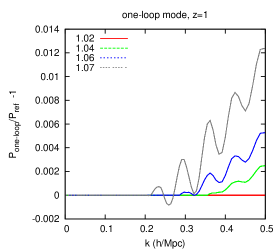
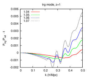
Figure 3: Convergence proof for the integration in momentum space in the the one-loop (left) and TRG (right) modes. The reference model has logstepx_min=1.001 in the one-loop case, or logstepx_min=1.02 in the TRG case.

In all integrals, we define some ultra-violet and infra-red cuts-off ($k_{\textrm{min}}$, $k_{\textrm{max}}$) besides which the power spectra are assumed to vanish. Moreover, below a scale $k_{L}$, we assume that the evolution of the spectrum remains strictly linear at all times: this means that for $k<k_{L}$, we set the $A$ coefficients to zero, in order to speed up the calculation. We checked that the results are well converged with the choices $k_{\textrm{min}}=10^{-4}h/$Mpc, $k_{L}=10^{-3}h/$Mpc, $k_{\textrm{max}}=10^{3}h/$Mpc.

4.5 Numerical instabilities

The main challenge in any implementation of the TRG algorithm is to keep numerical noise under control in the ultra-violet limit. Indeed, a small error in the tail of the power spectrum would be amplified by the recursion over time, and lead to exponential divergences. By the same phenomenon, a slightly non-smooth initial spectrum would produce non physical divergences. The smoothness of the spectrum is very difficult to control since it is passed in the form of tabulated values.

We checked that the divergences and wiggles observed in our first, straightforward implementation of the algorithm were only numerical artifacts. Indeed, we varied the size of time and wavenumber steps, and observed that these features propagated at a rate defined by the number of discrete steps, rather than by physical time.

In order to eliminate these numerical artifacts, we tried to implement several smoothing algorithms and several exponential cut-off functions in the small-scale linear power spectrum. Every time, some feature would finally propagate. By the very nature of the non-linear equations, as time goes by, any small error is amplified in huge proportions.

We solved this issue with an approach which is physically justified by the fact that during structure formation, mode coupling leads to a transfer of power from large scales to small scales, and not in the other direction. At each new time step, numerical artefact’s unavoidably affect the last four points in the list of discrete $k$ values (two points in the computation of the time derivative, plus two points in the calculation of the $A$ integrals). Hence, one can systematically throw away these last four points. In practice, this method (that we call “double escape”) consists in integrating the TRG equation only in a range $k_{\mathrm{L}}\leq k\leq k_{\mathrm{DE}}(\eta)$. The wavenumber $k_{\mathrm{DE}}(\eta)$ (where DE stands for double escape) coincides with $k_{\mathrm{max}}$ at initial time, and then decreases by discarding four more points in $k$-space at each half time step $\delta\eta/2$. Since a given wavenumber is impacted by the evolution of smaller wavenumbers only, our method cannot affect the final results. We checked it explicitly by changing the step sizes in $k$ space. Such a reduction means that we decrease $k_{\mathrm{DE}}(\eta)$ differently as a function of time, but the final results remain totally invariant. Simply, smaller step sizes allow to get results at a larger $k_{\mathrm{DE}}$ at $z=0$, starting from the same initial $k_{\mathrm{max}}$. In the released version, the default time steps are such that $k_{\mathrm{DE}}\sim 0.25h/$Mpc today. When the user asks for non-linear spectra at a given redshift, they are only written in output files up to the corresponding value of $k_{\mathrm{DE}}(\eta)$.

Note that when computing the $A$ integrals, the power spectra still need to be evaluated between $k_{\mathrm{DE}}(\eta)$ and $k_{\mathrm{max}}$, but the final results have a very weak dependence on $P_{ab}(k)$ in this range. We use a log-linear extrapolation of $P_{ab}(k)$ besides $k_{\mathrm{DE}}(\eta)$, based on an estimate of the logarithmic derivative in $k=k_{\mathrm{DE}}(\eta)$. We actually tried alternative extrapolation schemes (e.g. with constant second derivative in log-log space) and found that the final result is independent on the scheme (again, as a consequence of the fact that a wavenumber is only affected by its smaller neighbors).

We conclude that this “double escape” is a simple and robust way to keep numerical instabilities under control, leading to a “loss of information” on the smallest wavelengths, but introducing no bias in the final results.

Note that these problems arise when dealing with the full TRG equations. In its one-loop limit D1L, which will be seen below to provide excellent results, the integration over time is perfectly stable, and there is no need to throw points away.

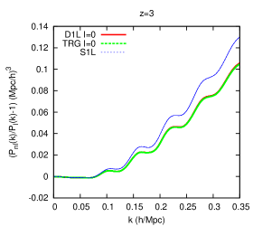
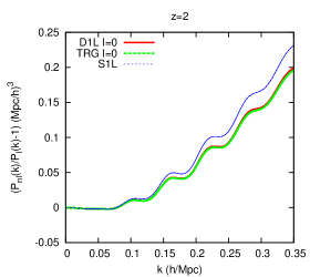
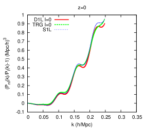
Figure 4: In an ideal EdS limit and at four different redshifts, comparison between the non-linear spectra computed with the standard one-loop S1L, dynamical 1-loop D1L and TRG methods. For the D1L and TRG case, we start the computation from exactly linear initial conditions at $z_{\rm ini}=35$ (with vanishing bispectrum), causing a residual difference with respect to the S1L method.

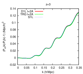
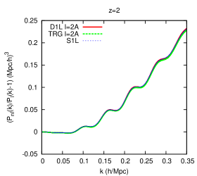
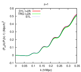
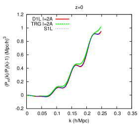
Figure 5: Same as previous figure, although for the D1L and TRG case we now start from an initial condition $I=2A$, which amounts in sharing the same assumptions as the S1L calculation.

5 Self-consistency checks in the exact EdS limit

The main purpose of this section is to test the agreement between the S1L and D1L methods. This check is more straightforward in a model without non-trivial growth factors related to $\Omega_{m}$ begin smaller than one, i.e. in the Einstein-De Sitter limit. Hence, for the results of this section, we modified our TRG/D1L module in order to enforce a perfect EdS evolution. This amounts in:

• replacing the actual matrix elements $\Omega_{2b}$ by $(3/2,-3/2)$,

• for D1L, replacing the exact growth functions by $g(\eta)=1$, $f(\eta)=1$.

The issue of initial conditions is crucial. The simplest choice consists in starting from exactly linear perturbations at $z=z_{\rm ini}$, i.e. from a $P_{11}(k)$ given by the linear density power spectrum, from $P_{22}(k)=P_{12}(k)=P_{11}(k)$, and from $I_{acd,bef}(k)=0$. Starting from such conditions at $z_{\rm ini}=35$, we obtain the 1-loop density power spectra named D1L in figure 4. They are actually smaller than S1L results, at all redshift and by several percents (at $k=0.25\,h$Mpc^-1 they predict non-linear spectra differing respectively by $1.2,1.5,2,5\%$ at $z=3,2,1,0$). This discrepancy actually decreases when we start the integration at a higher redshift. This suggests that the difference arises from neglecting any non-linear evolution before $z_{\rm ini}$. Indeed, the S1L method assumes that from $z\longrightarrow\infty$ till today, the modes have always evolved according to the newtonian equations in the EdS limit, with a linear growth factor proportional to $a$. This is of course an approximation, but in order to do a consistent comparison of the methods, we should also integrate the D1L and TRG equations starting from initial conditions reflecting the 1-loop evolution in the range $z\in[\infty,z_{\rm ini}]$, instead of linear initial conditions.

This amounts in taking the initial $P_{ab}(k)$ to be the one-loop spectra at $\eta=0$, and in computing $I_{acd,bef}(k)$ at $\eta=0$ at leading order in perturbation theory. However, one-loop corrections to the linear $P_{ab}(k)$ at $z\sim 35$ appear to be completely negligible in the range of interest (at least until $k\sim 1\,h$Mpc^-1), so sticking to the linear spectra makes no difference in practice (we checked this explicitely). This is not true as far as the initial bispectra are concerned: instead of $B=0$, we should use the tree-level bispectrum expression [3], computed at $z_{\rm ini}$ out of the linear power spectra. When plugged into the expression of $I_{acd,bef}(k)$, the tree-level bispectrum leads to a series of terms that we computed explicitely. We checked numerically that all terms are negligible with respect to the leading one, namely $I=2A$: so, for simplicity, we will approximate the tree-level expression of $I$ as $2A$. A more intuitive derivation of this result follows from observing equation (19). At very early time, the bispectrum is driven away from zero by the source $A_{acd,bef}$, so that

$$\partial_{\eta}I_{acd,bef}(k)\simeq 2e^{\eta}A_{acd,bef}(k)~{}.$$ (23)

Since at leading order in perturbation theory $A_{acd,bef}(k)$ is constant in time, this approximate evolution equation is solved by $I_{acd,bef}(k)=2e^{\eta}A_{acd,bef}(k)$, which corresponds to the initial condition $I_{acd,bef}(k)=2A_{acd,bef}(k)$ at $\eta=0$.

When adopting such initial conditions, the D1L results nicely coincide with S1L predictions, as can be seen in figure 5. This was of course expected on a purely analytical basis, but the agreement proves that the two methods are correctly implemented numerically.

The most important result of this paper is already visible in Figures 4 and 5: on the scales displayed in the figures, the TRG curves are always very close to their D1L counterpart with the same initial conditions, at least for $z\geq 2$. At $z=1$, differences at the level of half-a-percent start to appear. At $z=0$ one can see clear differences of 1 or 2% on the scales corresponding to BAO dips: the TRG smoothes BAOs more than 1-loop approaches. However, this difference between D1L and TRG results remains small, especially in regard of the large increase in computing time in the TRG case. Since in a realistic scenario the growth of structure is suppressed with respect to the EdS case, this conclusion is likely to hold even better in $\Lambda$CDM, as we shall see below.

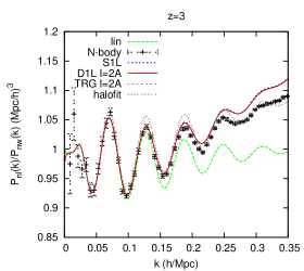
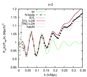
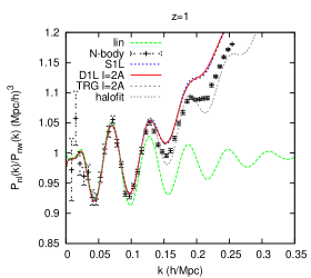
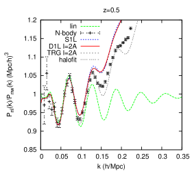
Figure 6: Matter power spectrum divided by a smooth one [15] for $z=3,2,1,0.5$ obtained with five different methods: N-body simulations [8], TRG method, standard one-loop S1L, dynamical one-loop D1L, and finally HALOFIT [2]. Here we employed non-physical initial conditions $I=2A$ in order to check the agreement between D1L and S1L results, but we know that these results cannot be trusted.

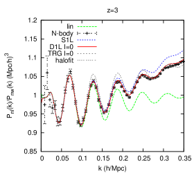
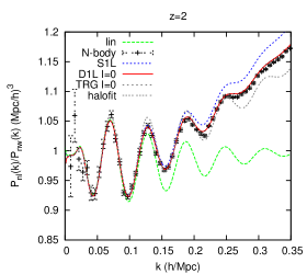
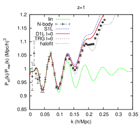
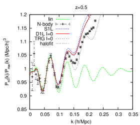
Figure 7: These figures contain our main results. The matter power spectrum divided by a smooth one [15] for $z=3,2,1,0.5$ obtained with five different methods: N-body simulations [8], TRG method, standard one-loop S1L, dynamical one-loop D1L, and finally HALOFIT [2]. In contrast with the previous figure, we now assume linear initial conditions ar $z_{\rm ini}$. This assumption appears to provide excellent results on all displayed scales till $z=2$, and still better predictions than halofit at $z=1,0$.

6 Results for $\Lambda$CDM and comparison with N-body simulations

We finally ran our code for a $\Lambda$CDM model, in order to check that the findings of the previous section remain true, namely: (i) the fact that the D1L method with $I=2A$ matches S1L predictions (despite the fact that D1L treats in a more exact way the impact of $\Omega_{m}<1$ at early time due to the small radiation density, and the consequence of late $\Lambda$ domination for the time evolution of the density and velocity linear growth factors), and (ii) the fact that TRG results do not improve significantly over one-loop calculations.

Also, in order to evaluate the precision of each method, we wish to compare semi-analytic predictions with very accurate N-body simulations, leading to a density power spectrum with a good resolution in $k$-space, and a small sampling variance on mildly non-linear scales, hopefully quantified by an error bar. Such power spectra can only be obtained by running several simulations in a very large box, and computing the mean and variance of the resulting collection of spectra. Simulations with these characteristics have been presented in several papers including Refs. [5, 8, 16]. In Refs. [5, 16], the initial linear spectrum was inferred from analytical fitting formulas, which are not accurate at the per-cent level. We prefer to use the recently published simulations of Sato et al. [8], based on an initial spectrum computed with CAMB. These authors performed a large number of high-quality simulations, leading to sub-percent level statistical errors, and to a very good matching between linear and N-body spectra for wavenumbers in the range $[0.05-0.1]h$/Mpc.

We show in figures 6, 7 a comparison between those results and the non-linear spectra obtained with the one-loop (S1L and D1L), TRG and HALOFIT semi-analytical methods. All spectra are computed for a model with $h=0.71$, $\Omega_{\Lambda}=0.735$, $\Omega_{b}=0.0448$, $N_{\rm eff}=3.04$, $T_{\rm cmb}=2.726$K, $n_{s}=0.963$ and $\sigma_{8}=0.80$.

Like in the previous section, we have to face the crucial issue of initial conditions. We know that starting from the tree-level bispectrum, equivalent to $I=2A$, amounts in doing the same assumption as in the S1L calculation: it assumes that the bispectrum has grown like in an ever-matter dominated universe, containing a single presureless species described by Newtonian equations. Actually, most recent N-body simulations (including the one quoted here) also share this assumption. Indeed, their initial conditions are set by a 2LPT (2nd-order Lagrange Perturbation Theory) algorithm, designed in such way to minimize transient effects. This result is achieved precisely by assuming a tree-level initial bispectrum at initial time. Hence, the choice $I=2A$ is the proper one for comparing D1L or TRG results both with S1L predictions and with N-body results.

We show in figure 6 the D1L and TRG results obtained from such initial conditions. The S1L and D1L method are again in very good agreement. We could expect D1L and S1L to depart from each other at $z\leq 1$, when $\Lambda$ domination leads to non-trivial growth factor which render the expansion of eq. (4) only approximate. This difference can be observed at $z=0.5$ on the scale $k=0.125\,h$/Mpc corresponding to a maximum in the BAOs. However, it is only a sub-percent effect, which confirms the results of Ref. [6], figure 7, in which a similar test was presented. As in the previous section, the TRG results are very close to the S1L ones , even at $z=0.5$. All three methods tend to overestimate non-linear corrections to the density power spectrum: this trend was already well-known for calculations limited to one-loop, and our result shows that TRG results make roughly the same error. Percent precision is nevertheless achieved until $k\sim 0.2\,h$Mpc^-1 for $z\geq 2$, or until $k\sim 0.14\,h$Mpc^-1 at $z=1$.

For comparison, the results obtained when starting from $I=0$, which are presented in figure 7, seem to be in much better agreement with N-body simulations. Note that earlier comparisons shown in Ref. [6, 12, 7, 13, 14] were based on the same assumptions. However, this comparison is not fully self-consistent, since it relies on different choices of initial conditions in the different methods. Hence, the better agreement observed in this plot is likely to be purely coincidental.

7 Discussion

In this work, we compared a few semi-analytical methods to the recent accurate N-body simulations of Sato et al. [8] and to standard 1-loop perturbation theory. We released these methods in the form of a C module, named trg.c and integrated in the Boltzmann code CLASS, version 1.2. The first method is the Time Renormalization Group (TRG) proposed by M. Pietroni. The second method, named here D1L (Dynamical 1-Loop) and based on the same approach, leads to nearly identical results on scales of interest, with a much smaller computing time. We have explained in this paper our approach for dealing with numerical instabilities, and for optimizing the algorithm. We have also presented some convergence tests proving its reliability. This release allows any cosmologist to compute easily an approximate non-linear spectrum (from first principles, rather than with fitting formulas), while until now this task was only accessible to a few specialists.

Differences between TRG and D1L are visible at low redshift, but they remain very small on scales of interest. This shows that the partial resumation of diagrams beyond one loop in the TRG method improves one-loop results by a negligible amount, for a much larger computing time. Hence, the one-loop limit of the TRG equations (namely, the D1L scheme) is preferable in practice.

The D1L algorithm is a fast and practical tool for obtaining one-loop results for the density/velocity power spectra (and tree-level results for the bispectra), even for non-trivial cosmological models or in presence of an arbitrary initial bispectrum. There are several ways to incorporate such assumptions in one-loop calculations, but in the D1L equations, this flexibility is present from the beginning. In this paper, we used this opportunity for showing the importance of assumptions concerning the initial bispectrum. In our universe, the non-linearity of the gravitational equations is sufficient to induce a tiny bispectrum even at very high redshift on cosmological scales of interest in this paper. At any given initial redshift, this bispectrum is small enough to be well approximated by a tree-level calculation, but nevertheless large enough to impact results at small redshift by several percents. This observation is consistent with previous studies of initial conditions for N-body simulations. In particular, the 2LPT method has been developed in order to deal with transient effects in simulations [17], i.e. in order to remove spurious decaying modes by implementing initial conditions infered from second-order Lagrangian perturbation theory, including an initial tree-level bispectrum. However, this fact had been overlooked in the context of TRG calculations. We have shown that previous claims that TRG results improve over one-loop predictions were the consequence of neglecting this initial bispectrum. When using the same initial bispectrum in all methods, the difference between S1L, D1L and TRG results almost disappears.

It is beyond the scope of this paper to discuss to which extent the initial conditions assumed in the S1L method and in N-body simulations offer a sufficiently realistic description of the actual universe. The fact that at high redshift baryons, cold dark matter and radiation perturbations do not share the same transfer functions and do not obey exactly to the growing mode solution means that in principle, one should implement some amount of “physical transient effects” in the initial conditions of both N-body simulations and renormalisation algorithms. The authors of [18] have already shown the importance of treating baryons separately from cdm when performing non-linear calculations. To our knowledge, the impact of early baryon and radiation perturbations on the calculation of the initial bispectrum (to be passed to N-body initial condition generators) has not been quantified accurately. We speculate that the D1L algorithm described in this paper could be a convenient tool for computing realistic high-redshift bispectra, and we leave this for future studies.

Appendix A From Boltzmann to continuity and Euler equation

Let’s start by considering a large set of particles only interacting through gravitation. In order to lighten slightly this presentation, let us omit the $m$ subscript for the moment. For each particle (CDM or baryon) the equation of motion is given in terms of its proper time $t$, velocity $\mathbf{v}$ and position $\mathbf{r}$:

$$\frac{\text{d}\mathbf{v}}{\text{d}t}=-\frac{\partial\phi}{\partial\mathbf{r}},$$ (24)

where $\phi$ is the Newtonian potential induced by the local mass density $\rho(\mathbf{r})$,

$$\phi(\mathbf{r})=G\int\text{d}^{3}\mathbf{r}^{\prime}\frac{\rho(\mathbf{r}^{\prime})}{|\mathbf{r}^{\prime}-\mathbf{r}|}.$$ (25)

This set of particles is however sitting in an expanding universe. The gravitational collapse consists in studying departures from the homogeneous Hubble expansion. It is then useful to redefine the variables of position and momentum with respect to the comoving ones. The physical space coordinates $\mathbf{r}$ relate to the comoving space coordinates $\mathbf{x}$ through $\mathbf{r}\equiv a(\tau)\mathbf{x}$. We can define the density perturbation $\delta(\mathbf{x},\tau)$, the peculiar velocity $\mathbf{u}(\mathbf{x},\tau)$ and the cosmological gravitational potential $\Phi(\mathbf{x},\tau)$ by

$$\rho(\mathbf{x},\tau) \equiv\bar{\rho}(\tau)[1+\delta(\mathbf{x},\tau)],$$ (26)

$$\mathbf{v}(\mathbf{x},\tau) \equiv\mathcal{H}\mathbf{x}+\mathbf{u}(\mathbf{x},\tau),$$ (27)

$$\mathbf{\phi}(\mathbf{x},\tau) \equiv-\frac{1}{2}\frac{\partial\mathcal{H}}{\partial\tau}\mathbf{x}^{2}+\Phi(\mathbf{x},\tau).$$ (28)

The Einstein equations lead in the sub-Hubble, weak gravitational field limit to the Poisson equation:

$$\nabla^{2}\Phi(\mathbf{x},\tau) =-\frac{3}{2}\mathcal{H}^{2}\sum_{i}\Omega_{i}(\tau)\delta_{i}(\mathbf{x},\tau).$$ (29)

Defining the momentum $\mathbf{p}=am\mathbf{u}$, eq. (24) now reads:

$$\frac{\text{d}\mathbf{p}}{\text{d}\tau}=-am\nabla\Phi(\mathbf{x}).$$ (30)

One finally write the collisionless Boltzmann equation for the phase-space density $f(\mathbf{x},\mathbf{p},\tau)$ in its full form:

$$\frac{\text{d}f}{\text{d}\tau} =\frac{\partial f}{\partial\tau}+\frac{\mathbf{p}}{ma}\cdot\nabla f-am\nabla\Phi\cdot\frac{\partial f}{\partial\mathbf{p}}.$$ (31)

The non-linearity of this equation is induced by gravitational back-reaction, described by the Poisson equation. This equation is obviously hard to solve due to its high dimensionality, which can however be reduced by taking the momenta of the distribution $f(\mathbf{x},\mathbf{p},\tau)$, and by truncating such an expansion at some order, if this can be physically justified. Let us define the first three momenta as:

$$\int\text{d}^{3}\mathbf{p}~{}f(\mathbf{x},\mathbf{p},\tau)~{} \equiv ~{}\rho(\mathbf{x},\tau),$$ (32)

$$\int\text{d}^{3}\mathbf{p}~{}\frac{\mathbf{p}}{am}f(\mathbf{x},\mathbf{p},\tau)~{} \equiv ~{}\rho(\mathbf{x},\tau)\mathbf{u}(\mathbf{x},\tau),$$ (33)

$$\int\text{d}^{3}\mathbf{p}~{}\frac{p_{i}p_{j}}{a^{2}m^{2}}f(\mathbf{x},\mathbf{p},\tau)~{} \equiv ~{}\rho(\mathbf{x},\tau)u_{i}u_{j}(\mathbf{x},\tau)+\sigma_{ij}(\mathbf{x},\tau).$$ (34)

Taking the zeroth moment of eq. (31) leads to the continuity equation:

$$\frac{\partial\delta(\mathbf{x},\tau)}{\partial\tau}+\nabla\cdot{[1+\delta(\mathbf{x},\tau)]\mathbf{u}(\mathbf{x},\tau)}=0,$$ (35)

while the first moment gives (after subtracting $\mathbf{u}(\mathbf{x},\tau)$ times (35)) the Euler equation:

$$\frac{\partial u_{i}(\mathbf{x},\tau)}{\partial\tau}+\mathcal{H}(\tau)u_{i}(\mathbf{x},\tau)+\left(\mathbf{u}(\mathbf{x},\tau)\cdot\nabla\mathbf{u}(\mathbf{x},\tau)\right)_{i}=-\nabla_{i}\Phi(\mathbf{x},\tau)-\frac{1}{\rho}\nabla_{j}\sigma_{ij}.$$ (36)

One usually takes the anisotropic pressure $\sigma_{ij}$ to be equal to zero. This approximation is excellent not just for baryons (they interact, so they are considered as a perfect fluid with no shear), but also for cold dark matter. Indeed, CDM particles have no interactions but a tiny velocity dispersion, leading to negligible anisotropic pressure on scales where CDM can be represented by a single-flow distribution. In the range of linear and quasi-linear scales considered here, this approximation is valid.

With such considerations, we can safely use from now on the $\delta_{m}$ notation for both baryons and CDM. The Poisson equation (29) can be cast into a more convenient form:

$$\nabla^{2}\Phi(\mathbf{x},\tau) =-\frac{3}{2}\mathcal{H}^{2}\Omega_{m}(\tau)\delta_{m}(\mathbf{x},\tau)\left(1+\sum_{i\neq b,c}\frac{\Omega_{i}\delta_{i}}{\Omega_{m}\delta_{m}}\right),$$ (37)

where in $i$ stands for photons and neutrinos (relativistic or not). It can be seen from eq. (36) that the curl part of the velocity field decouples and is suppressed by the universe expansion. The equations can then be reformulated in terms of the density perturbation and the velocity divergence $\theta=\nabla\cdot\mathbf{u}$. Furthermore, to have a better understanding of the mode coupling induced by the non-linearity, we transform the equation into Fourier space, with the following convention:

$$A(\mathbf{k},\tau) =\frac{1}{(2\pi)^{3}}\int\text{d}^{3}\mathbf{x}e^{-i\mathbf{k}\cdot\mathbf{x}}A(\mathbf{x},\tau).$$ (38)

In Fourier space, the equations governing the matter field reduce to

$$\frac{\partial\delta_{m}(\mathbf{k},\tau)}{\partial\tau}+\theta_{m}(\mathbf{k},\tau) =-\int\text{d}^{3}\mathbf{q}\text{d}^{3}\mathbf{p}\delta_{D}(\mathbf{k}-\mathbf{p}-\mathbf{q})\alpha(\mathbf{p},\mathbf{q})\theta_{m}(\mathbf{p},\tau)\delta_{m}(\mathbf{q},\tau),$$ (39)

$$\frac{\partial\theta_{m}(\mathbf{k},\tau)}{\partial\tau}+\mathcal{H}(\tau)\theta_{m}(\mathbf{k},\tau)$$

$$+\frac{3}{2}\mathcal{H}(\tau)^{2}\sum_{i}\Omega_{i}(\tau)\delta_{i}(\mathbf{k},\tau) =-\int\text{d}^{3}\mathbf{q}\text{d}^{3}\mathbf{p}\delta_{D}(\mathbf{k}-\mathbf{p}-\mathbf{q})\beta(\mathbf{p},\mathbf{q})\theta_{m}(\mathbf{p},\tau)\theta_{m}(\mathbf{q},\tau),$$ (40)

where the kernels $\alpha$ and $\beta$ encoding the mode coupling are defined as:

$$\alpha(\mathbf{p},\mathbf{q}) \equiv\frac{(\mathbf{p}+\mathbf{q})\cdot\mathbf{p}}{p^{2}},\hskip 56.9055pt\beta(\mathbf{p},\mathbf{q})\equiv\frac{(\mathbf{p}+\mathbf{q})^{2}(\mathbf{p}\cdot\mathbf{q})}{2p^{2}q^{2}}.$$ (41)

Appendix B Structure of the trg.c module in CLASS

As explained in [9], CLASS is organized in eleven modules. The role of the ninth module nonlinear.c is to evaluate the non-linear power spectra according to the method chosen by the user. In the current version CLASS v1.1, the nonlinear.c module can optionally call the trg.c module described in this paper, in one out of three modes (non linear = test-linear, one-loop or trg) already described in subsection 4.2), and with a set of precision parameters. After the execution of the trg.c module, the code is ready to write in output files the non-linear density, velocity and cross spectra at different redshifts chosen by the user.

The trg.c module consists of several functions. The most important one, trg_init(), is called from the nonlinear.c module. Its goal is to compute the non-linear power spectrum from a given starting redshift and linear power spectrum previously computed by the spectra.c module.

The trg_init() routine first defines relevant step sizes in $\eta$ space and in $k$ space. For the latter, it calls the two functions trg_logstep1_k() and trg_logstep2_k(). The $k$ steps are defined in such way to keep a high resolution in the baryon-oscillation zone, and a reasonably small number of steps on other scales. Since these steps are relevant for the double escape procedure defined previously, one might want to be cautious while modifying them.

The initial density spectrum $P_{11}$ is taken directly from the spectra.c module. The initial velocity and cross spectra $P_{22}$ and $P_{12}$ are computed by evaluating a finite difference between $P_{11}$ at $\eta_{ini}\pm\epsilon$. At the starting redshift, three-points correlating functions (bispectra) are assumed to be zero, so all $I$’s defined in eq. (18) are initially zero.

The integration of the TRG equations (full equations in trg mode, simplified equations in the other two modes) is then performed. At each step in the trg mode, or only once in the one-loop mode, trg_init() calls trg_integrate_xy_at_eta to perform explicitly the integrals in $(x,y)$ space and find each of the 14 $A$ factors. This last function evaluates each of the 14 integrands at each $(x,y)$ point by calling the function trg_A_arg_trg() (or trg_A_arg_one_loop()).

After the execution of the trg.c module, the non-linear spectra are stored in a structure nonlinear associated with the nonlinear.c module. They can be evaluated at any value of $k$ and $z$ by calling the function nonlinear_pk_at_k_and_z(). Instead, all values at a given $z$ are returned by the function nonlinear_pk_at_z(). The output module output.c actually calls this last function in order to write the final results in separate files for the density, velocity and cross spectra.

References

- [1] S. Hannestad, “Can cosmology detect hierarchical neutrino masses?,” Phys.Rev. D67 (2003) 085017, astro-ph/0211106.
- [2] The Virgo Consortium Collaboration, R. Smith et al., “Stable clustering, the halo model and nonlinear cosmological power spectra,” Mon.Not.Roy.Astron.Soc. 341 (2003) 1311, astro-ph/0207664.
- [3] F. Bernardeau, S. Colombi, E. Gaztanaga, and R. Scoccimarro, “Large-scale structure of the universe and cosmological perturbation theory,” Phys. Rept. 367 (2002) 1–248, astro-ph/0112551.
- [4] M. Crocce and R. Scoccimarro, “Renormalized cosmological perturbation theory,” Phys.Rev. D73 (2006) 063519, astro-ph/0509418.
- [5] M. Crocce and R. Scoccimarro, “Nonlinear Evolution of Baryon Acoustic Oscillations,” Phys.Rev. D77 (2008) 023533, 0704.2783.
- [6] M. Pietroni, “Flowing with Time: a New Approach to Nonlinear Cosmological Perturbations,” JCAP 0810 (2008) 036, 0806.0971.
- [7] J. Carlson, M. White, and N. Padmanabhan, “A critical look at cosmological perturbation theory techniques,” Phys.Rev. D80 (2009) 043531, 0905.0479.
- [8] M. Sato and T. Matsubara, “Nonlinear Biasing and Redshift-Space Distortions in Lagrangian Resummation Theory and N-body Simulations,” 1105.5007.
- [9] J. Lesgourgues, “The Cosmic Linear Anisotropy Solving System (CLASS) I: Overview,” 1104.2932.
- [10] D. Blas, J. Lesgourgues, and T. Tram, “The Cosmic Linear Anisotropy Solving System (CLASS) II: Approximation schemes,” 1104.2933.
- [11] V. Springel, “The Cosmological simulation code GADGET-2,” Mon.Not.Roy.Astron.Soc. 364 (2005) 1105–1134, astro-ph/0505010.
- [12] J. Lesgourgues, S. Matarrese, M. Pietroni, and A. Riotto, “Non-linear Power Spectrum including Massive Neutrinos: the Time-RG Flow Approach,” JCAP 0906 (2009) 017, 0901.4550.
- [13] G. D’Amico and E. Sefusatti, “The nonlinear power spectrum in clustering quintessence cosmologies,” 1106.0314.
- [14] S. Anselmi, G. Ballesteros, and M. Pietroni, “Non-linear dark energy clustering,” 1106.0834.
- [15] D. J. Eisenstein and W. Hu, “Baryonic features in the matter transfer function,” Astrophys.J. 496 (1998) 605, astro-ph/9709112.
- [16] J. Kim, C. Park, I. Gott, Richard, and J. Dubinski, “The Horizon Run N-body Simulation: Baryon Acoustic Oscillations and Topology of Large Scale Structure of the Universe,” Astrophys.J. 701 (2009) 1547–1559, 0812.1392.
- [17] M. Crocce, S. Pueblas, and R. Scoccimarro, “Transients from Initial Conditions in Cosmological Simulations,” Mon.Not.Roy.Astron.Soc. 373 (2006) 369–381, astro-ph/0606505.
- [18] G. Somogyi and R. E. Smith, “Cosmological perturbation theory for baryons and dark matter I: one-loop corrections in the RPT framework,” Phys.Rev. D81 (2010) 023524, 0910.5220.