Neutrino Signatures on the High Transmission Regions of the Lyman-$\alpha$ Forest

Abstract

We quantify the impact of massive neutrinos on the statistics of low density regions in the intergalactic medium (IGM) as probed by the Lyman-$\alpha$ forest at redshifts $z=2.2$–$4$. Based on mock but realistic quasar (QSO) spectra extracted from hydrodynamic simulations with cold dark matter, baryons and neutrinos, we find that the probability distribution of weak Lyman-$\alpha$ absorption features, as sampled by Lyman-$\alpha$ flux regions at high transmissivity, is strongly affected by the presence of massive neutrinos. We show that systematic errors affecting the Lyman-$\alpha$ forest reduce but do not erase the neutrino signal. Using the Fisher matrix formalism, we conclude that the sum of the neutrino masses can be measured, using the method proposed in this paper, with a precision smaller than 0.4 eV using a catalog of 200 high resolution (S/N$\sim$100) QSO spectra. This number reduces to 0.27 eV by making use of reasonable priors in the other parameters that also affect the statistics of the high transitivity regions of the Lyman-$\alpha$ forest. The constraints obtained with this method can be combined with independent bounds from the CMB, large scale structures and measurements of the matter power spectrum from the Lyman-$\alpha$ forest to produce tighter upper limits on the sum of the masses of the neutrinos.

1 Introduction

Neutrino oscillation experiments revealed that neutrinos are not massless particles. Since then a major effort has been dedicated to measure or constrain neutrino masses. Current laboratory bounds constrain the electron neutrino mass to $m_{\nu_{e}}<2.05$ eV (Lobashev, 2003; Kraus et al., 2005). Cosmological bounds for the sum of all neutrino masses are still significantly stronger: constraints from WMAP7 alone yield $\Sigma_{i}m_{\nu_{i}}<1.3$ eV (Komatsu et al., 2009), while combined with large scale structure (LSS) measurements they constraint the mass to $\Sigma_{i}m_{\nu_{i}}<0.3$ eV (Wang et al., 2005; Thomas, Abdalla, & Lahav, 2010; Gonzalez-Garcia, Maltoni, & Salvado, 2010; Reid et al., 2010; de Putter et al., 2012; Xia et al., 2012) . The tightest $2\sigma$ upper limit of $\Sigma_{i}m_{\nu_{i}}<0.17$ eV, is obtained by combining cosmic microwave background (CMB) results, LSS and Lyman-$\alpha$ forest(Seljak, Slosar, & McDonald, 2006) data sets (see (Abazajian et al., 2011) for a summary of current and future neutrino mass constrains). Among all the different observables the Lyman-$\alpha$ forest is particularly constraining since it probes structures over a wide range of redshift, in a mildly non-linear regime and at small scales where the neutrino signature is present (Lesgourgues & Pastor, 2006; Rauch, 1998; Meiksin, 2009).

The dynamics of cosmological neutrinos is very different from that of the dominant cold dark matter (CDM) component. The large velocity dispersion of neutrinos suppresses their power spectrum of density fluctuations at small scales, making the shape of the total power spectrum a potential probe of neutrino masses.

Previous studies have addressed the role of neutrinos in dark matter halos (Singh & Ma, 2003; Ringwald & Wong, 2004; Villaescusa-Navarro et al., 2011), LSS (Ma & Bertschinger, 1994; Brandbyge et al., 2008; Brandbyge & Hannestad, 2009, 2010; Brandbyge et al., 2010; Marulli et al., 2011; Bird, Viel, & Haehnelt, 2012) and the intergalactic medium (IGM) (Viel, Haehnelt, & Springel, 2010), using both linear theory and N-body/hydrodynamic techniques for the non-linear regime. It has been shown that on scales of 1-10 $h^{-1}$Mpc the non-linear suppression is redshift, scale and mass dependent in a way that is different from a naive extrapolation of linear theory.

Figure 1: Linear matter power spectra for different neutrino masses at $z=0$ (upper lines) and $z=3$ (bottom lines). The inner panel shows the linear (solid lines) and non-linear (dotted lines) matter power spectrum at $z=3$ normalized to the case without neutrinos. On scales $k<0.03~{}h$ ${\rm Mpc^{-1}}$ changes in the non-linear power spectra are driven by the differences in the linear power spectra.

In this paper we study the effect of massive neutrinos on the properties of low density regions or voids in the intergalactic medium (IGM). Neutrinos have only a mild effect on dark matter halos (Singh & Ma, 2003; Ringwald & Wong, 2004; Villaescusa-Navarro et al., 2011), since their large velocity dispersion prevents their clustering on small scales. In contrast, we find that the impact of neutrinos on void properties is much stronger. Voids are relatively empty regions with $\delta=\rho_{m}/\bar{\rho}_{m}-1$ ranging from almost $-1$ in their cores to $\sim-0.7$ at radii $10-20$ Mpc at $z=0$ (Colberg et al., 2008). By solving the dynamical equations for an isolated spherical top-hat underdense perturbation, we find that neutrinos modify the evolution of underdense regions by making them smaller and denser. Neutrinos contribute to the interior mass of the underdense region delaying the rate at which CDM is being evacuated from its interior and slowing down the velocity of the shell surrounding it. We find that the linearly extrapolated density contrast when the underdense region enters into its non-linear phase decreases by $\sim 10\%$ for neutrinos with $\Sigma_{i}m_{\nu_{i}}\sim 1$ eV. Using the analytic model presented in (Sheth & van de Weygaert, 2004) we find that the statistics of voids depend on both $\sigma_{8}$ and $\Sigma_{i}m_{\nu_{i}}$. Lyman-$\alpha$ voids and their dependence on other cosmological parameters have been investigated in (Viel, Colberg, & Kim, 2008). Here we focus on the dependence of void properties on the sum of the neutrino masses. We consider the Lyman-$\alpha$ signature of low density regions, and introduce a new and simple statistical tool (note that a similar observable was already studied in (Miralda-Escudé et al., 1996; Fan et al., 2002)) that samples most of the IGM volume and appears to be highly sensitive to neutrino masses.

2 Numerical Method

Name	$\Sigma_{i}m_{\nu_{i}}$ (eV)	$\sigma_{8}$ ($z=0$)	$N_{\mathrm{CDM}}^{1/3}$	$N_{\mathrm{b}}^{1/3}$	$N_{\nu}^{1/3}$
S0	$0.0$	$0.877$	$512$	$512$	$0$
S0+	$0.0$	$0.928$	$512$	$512$	$0$
S0-	$0.0$	$0.828$	$512$	$512$	$0$
S3	$0.3$	$0.948$	$512$	$512$	$0$
S3+	$0.3$	$0.877$	$512$	$512$	$0$
S3-	$0.3$	$0.807$	$512$	$512$	$0$
S5	$0.5$	$0.755$	$512$	$512$	$0$
S6	$0.6$	$0.732$	$512$	$512$	$0$
S6+	$0.6$	$0.877$	$512$	$512$	$0$
S7	$0.7$	$0.709$	$512$	$512$	$0$
LR0	$0.0$	$0.877$	$448$	$448$	$0$
LR6	$0.6$	$0.732$	$448$	$448$	$0$
P0	$0.0$	$0.877$	$512$	$512$	$512$
P6	$0.6$	$0.732$	$512$	$512$	$512$

Table 1: Summary of the N-body/hydrodynamic parameters of the simulations. The cosmological parameters are the same for all simulations and are given in the text. $\Omega_{\rm M}=\Omega_{\rm cdm}+\Omega_{\rm b}+\Omega_{\nu}$ is kept constant. $N_{\mathrm{CDM}}$, $N_{\mathrm{b}}$ and $N_{\nu}$ correspond to the number of CDM, baryon and neutrino particles, respectively. All the simulations except P0 and P6 are based on the Fourier space implementation of neutrinos (see text).

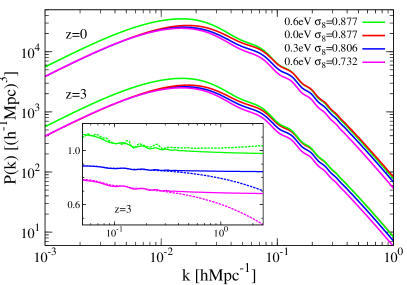
Our mock quasar spectra are based on cosmological simulations run with the TreePM-SPH code GADGET-3 (Springel, 2005). The code has been extended to include neutrinos either by solving their potential on the mesh or by representing them as discrete particles (Viel, Haehnelt, & Springel, 2010). Here, we use primarily the first implementation and refer the reader to (Marulli et al., 2011; Brandbyge et al., 2008; Brandbyge & Hannestad, 2009) for a critical comparison of the two methods and also for comparison with another new method Ali-Haïmoud & Bird (2012). Our simulations consist of $2\times 512^{3}$ CDM plus gas particles sampling a periodic box of $512~{}h^{-1}$Mpc. We adopt a flat $\Lambda$CDM background with cosmological parameters $\Omega_{\rm CDM}+\Omega_{\nu}=0.25$, $\Omega_{\Lambda}=0.7$, $\Omega_{b}=0.05$, $h=0.7$ and $n_{\rm s}=1$. We consider three degenerates neutrino species with a total mass of $\Sigma_{i}m_{\nu_{i}}=0.0,0.3$ and $0.6$ eV. The initial power spectra of most of our simulations, produced with CAMB, are normalized for all neutrino masses at a wavenumber $2\times 10^{-3}h~{}{\rm Mpc^{-1}}$, corresponding to the scale constrained by CMB data. This produces different values of $\sigma_{8}=0.877,~{}0.806$ and $0.732$ at $z=0$ for the models with $\Sigma_{i}m_{\nu_{i}}=0.0,~{}0.3$ and $0.6$ eV, respectively (see Fig. 1). Our initial conditions are generated at $z=49$. A summary of the different simulations we carried out is shown on table 1.

Figure 2: Real space distribution of the baryon density contrast, $\rho_{b}/\overline{\rho}_{b}$ (top panel), and the peculiar velocity, $V_{p}$ (middle), along a random line-of-sight (RLOS). In the bottom panel we plot the transmitted flux $F=e^{-\tau}$, in units of the mean flux $\langle F\rangle$, in redshift space.

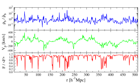
For each simulation we consider snapshots at redshifts $z=2.2$ and $z=4$ that bracket the range of interest for the observed Lyman-$\alpha$ forest in quasar spectra from ground-based telescopes. For each snapshot we sample 4500 random line-of-sights (RLOSs) uniformly distributed along each $x,y$ or $z$ direction. For each RLOS we extract the baryon density contrast $\rho_{b}(r)/\overline{\rho}_{b}$ and the peculiar velocity $V_{p}(r)$ along the line-of-sight and then compute the transmitted flux $e^{-\tau(u)}$ in redshift space (with $u$ in ${\rm km~{}s^{-1}}$), where $\tau$ is the Lyman-$\alpha$ optical depth, by using the Fluctuating Gunn Peterson Approximation:

$$\tau(u)=A\int_{-\infty}^{+\infty}dx~{}\delta[u-x-V_{p}(x)]~{}\bigg{(}\frac{\rho_{b}(x)}{\overline{\rho}_{b}}\bigg{)}^{1.6},$$ (1)

where $x=H(z)r/(1+z)$ is the redshift space coordinate and $A$ is a factor that depends on the global thermal history of the IGM (Croft et al., 2002),

$$A=0.433\bigg{(}\frac{1+z}{3.5}\bigg{)}^{6}\bigg{(}\frac{\Omega_{b}h^{2}}{0.02}\bigg{)}^{2}\bigg{(}\frac{0.65}{h}\bigg{)}\bigg{(}\frac{3.68H_{0}}{H(z)}\bigg{)}\times$$

$$\bigg{(}\frac{1.5\times 10^{-12}s^{-1}}{\Gamma_{HI}}\bigg{)}\bigg{(}\frac{6000K}{T_{0}}\bigg{)}^{0.7},$$ (2)

with $\Gamma_{HI}$ being the hydrogen photoionization rate. The power-law index in the scaling with $\rho_{b}/\overline{\rho}_{b}$ arises from the equation of state for the IGM temperature, $T=T_{0}(\rho_{b}/\overline{\rho}_{b})^{\alpha}$ (Hui & Gnedin, 1997), with $\alpha\approx 0.6$. In all our calculations we adopt $T_{0}=10^{4}$ K and choose $\Gamma_{HI}$ such that the mean flux over the whole set of RLOS reproduce the observed mean flux at redshift $z$ (Miralda-Escudé et al., 1996) $\langle F\rangle=e^{-\tau_{eff}(z)}$ with $\tau_{eff}(z)=0.0023(1+z)^{3.65}$ (Kim et al., 2007). We neglect the effects of thermal broadening. Finally, we smooth the flux over a scale of $1~{}h^{-1}$Mpc, which is larger than the Jeans length, to avoid sensitivity to substructure below the Jeans scale, which is affected by numerical resolution and astrophysical processes (e.g. feedback from galactic winds).

Figure 2 shows the baryon density contrast, $\rho_{b}/\overline{\rho}_{b}$, and peculiar velocity, $V_{p}$, extracted along a RLOS as a function of the comoving coordinate $r$ together with the corresponding transmitted flux $F=e^{-\tau}$ in redshift space, plotted in terms of the mean flux at redshift $z$.

3 Analysis of the simulations

We focus our analysis on the statistical properties of low density regions that are expected to produce weak absorption features. We define as void “region” a continuous domain in the transmitted flux profile which remains always above a given threshold. The higher the threshold, the lower the absorption in that region. For each RLOS we extract the transmitted flux from $\rho_{b}/\overline{\rho}_{b}$ and $V_{p}$ and count the number of regions above the selected threshold. This results in a statistical estimate of the low absorption contribution to the Lyman-$\alpha$ signal, and allows us to quantify the impact of neutrinos on those regions.

Figure 3: Probability distribution function (PDF) for the number of regions per path length of $100~{}h^{-1}$Mpc above a threshold of $F/\langle F\rangle=1.14$ (top), $1.70$ (bottom) as a function of $\Sigma_{i}m_{\nu_{i}}$ and $\sigma_{8}$ at $z=2.2$ (top) and $z=4$ (bottom). The PDFs have long tails with a very low probability that extend up to 10-12. The $\sigma_{8}-\Omega_{\nu}$ degeneracy is not perfect and can be broken by studying the spectra at different redshifts.

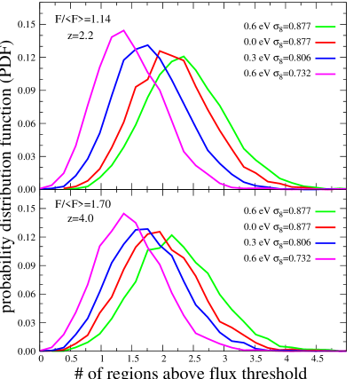
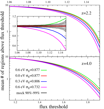
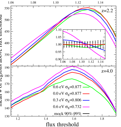
In Fig. 3 we plot the probability distribution function (PDF) for the number of regions per path length of $100~{}h^{-1}$Mpc above a threshold of $F/\langle F\rangle=1.14$ at redshift $z=2.2$ (top) and at redshift $z=4.0$ for a threshold $F/\langle F\rangle=1.70$ (bottom) for three different neutrino masses, $\Sigma_{i}m_{\nu_{i}}=0.0,~{}0.3,~{}0.6$ eV. The two numbers above are chosen taken into account two competing effects: on one side, the larger the value of $F/\langle F\rangle$ the larger the differences between the models. On the other side, the number of regions above the threshold drops rapidly as $F/\langle F\rangle$ increases, requiring a larger QSO spectra catalog to obtain converged results. By choosing the numbers above we make sure that differences are large enough having converged results. We have verified that these PDFs do not change if we increase the number of RLOS, i.e. our statistical sample of RLOS is large enough to reliably measure the PDF. Figure 3 shows that the neutrino mass has a significant impact on the mean of the distributions. In Fig. 4 we plot the mean of the distributions, i.e. the average number of regions per path length of $100~{}h^{-1}$Mpc above a given threshold, as a function of the threshold for the three different neutrino masses ($\Sigma_{i}m_{\nu_{i}}=0.0,~{}0.3,~{}0.6$ eV) at redshift $z=2.2$ (top) and $z=4.0$ (bottom). This shows clearly that the higher the threshold, the larger the differences between the various neutrino cosmologies. This is the expected neutrino signature as we discuss below.

Figure 4: Average number of regions per path length of $100~{}h^{-1}$Mpc as a function of flux threshold at redshift $z=2.2$ (top) and $z=4$ (bottom) for different neutrino masses and $\sigma_{8}$. The subplot in the upper panel shows the ratio between models with $\Sigma_{i}m_{\nu_{i}}\neq 0.0$ and the model with $\Sigma_{i}m_{\nu_{i}}=0.0$. The black error bars indicate the $90\%$ (interior tick marks) and $99\%$ (exterior tick marks) confident intervals for a mock catalog consisting of $200$ RLOS taken from the simulation with $(\Sigma_{i}m_{\nu_{i}}=0.0$ eV, $\sigma_{8}=0.877)$. Models with $\Sigma_{i}m_{\nu_{i}}=0.3,0.6$ and $\sigma_{8}=0.806,0.732$ respectively can be ruled out with a high significance by using a catalog of 200 QSO spectra.

We explicitly checked that relative differences between our neutrino models are numerically converged against mass and spatial resolution. Furthermore, we used the neutrino particle implementation (simulations P0 and P6 on table 1) and found the same trends in the neutrino signature as with the grid method, although relative differences between the different models are even slightly larger when we use the particle implementation. This is due to the fact that non-linear neutrino effects, such as phase mixing, are only properly captured by using the particle implementation. However, we note that the grid implementation in the mildly non-linear Lyman-$\alpha$  regime is fully justified since non-linear neutrinos effects should not be particularly important at those redshifts and at $k<1~{}h~{}{\rm Mpc^{-1}}$.

4 Systematic errors

The high transmissivity regions of the Lyman-$\alpha$ forest are prone to systematic errors such as those induced by the continuum fitting procedure and the signal to noise ratio ($S/N$) of the QSO spectrum. We have investigated whether these effects are able to spoil the neutrino signal. In particular, we have studied how the presence of systematic errors affects the differences between models (in terms of the average number of regions above the threshold at $z=2.2$), and their impact on the sensitivity to $\Omega_{\nu}$ of a catalog containing 200 QSO spectra.

We first focus our attention to the case without systematic errors. In the subplot of Fig. 4 we show the average number of regions per path length of $100~{}h^{-1}$Mpc as a function of the threshold at $z=2.2$ normalized to the neutrinoless model. The black error bars show the $90\%$ (interior tick marks) and $99\%$ (exterior tick marks) confident intervals for a mock catalog consisting of $200$ RLOS taken from the simulation with $(\Sigma_{i}m_{\nu_{i}}=0.0$ eV, $\sigma_{8}=0.877)$. We find that with a catalog consisting of $200$ QSO spectra (not affected by systematic errors) we can rule out models $(\Sigma_{i}m_{\nu_{i}}=0.3$ eV, $\sigma_{8}=0.806)$ and $(\Sigma_{i}m_{\nu_{i}}=0.6$ eV, $\sigma_{8}=0.732)$ with a high significance. Distinguishing models with the same $\sigma_{8}$ would require a larger QSO spectra catalog and combining results at different redshifts in order to disentangle the different redshift evolution of the models.

In order to study how systematic errors impact on our results, we have created a realistic mock catalog of high resolution QSO spectra. We have mimicked the continuum fitting errors by rescaling each flux pixel by the quantity $F_{i}/F_{max}$ ($F_{max}$ being the maximum value of the transmitted flux along the spectrum) as done by (McDonald et al., 2000); we considered a $S/N=100$ which is reasonable for UVES/VLT QSO spectra. Note that this treatment of the systematic errors induced by the continuum fitting is rather simplistic and conservative, and ideally one would like to put more refined models for the QSO continuum and generate a set of mock spectra that would be as close as possible to the observed one (for example by including the redshift distribution of the sources), however this is beyond the scope of the present paper.

Using this catalog, we have repeated the analysis described above and we show the results in Fig. 5. Two things can be pointed out from this figure. On one side, we find that the mean number of regions above a flux threshold is strongly affected by the Gaussian noise and by the bin size in the QSO spectra. This dependence can be easily understood considering that the Gaussian noise on a pixel can divide a single region above a threshold into two, and also by the fact that spurious regions will appear because the Gaussian noise can increase the value of the transmitted flux (ending up with a final value above the threshold) on a pixel which is below the threshold. On the other side, it turns out that, as expected, the differences between models become smaller as the QSO catalog $S/N$ drops. However, the remaining differences between models points out that neutrino effects are not erased by the presence of the systematics discussed in this Section. The subplot of Fig. 5 shows the ratio between the different models and the model with $\Sigma_{i}m_{\nu_{i}}=0.0$. The black error bars indicate the $90\%$ (interior tick marks) and $99\%$ (exterior tick marks) confident intervals for a mock catalog consisting of $200$ high resolution QSO spectra extracted from the simulation with $(\Sigma_{i}m_{\nu_{i}}=0.0$ eV, $\sigma_{8}=0.877)$. We find that with a high resolution catalog ($S/N=100$) consisting of 200 QSO spectra, models with $\Sigma_{i}m_{\nu_{i}}=0.0$ and $\sigma_{8}=0.877$ and $\Sigma_{i}m_{\nu_{i}}=0.6$ and $\sigma_{8}=0.732$ can be distinguished at a very high significance. The models with $\Sigma_{i}m_{\nu_{i}}=0.0$ and $\sigma_{8}=0.877$ and $\Sigma_{i}m_{\nu_{i}}=0.3$ and $\sigma_{8}=0.806$ can be distinguished with a lower significance, while in order to distinguish models with the same $\sigma_{8}$, a catalog with either more QSO spectra or higher $S/N$ value is needed.

In addition to the systematic errors arising from the noise in the spectra and the continuum fitting procedure, the presence of metal lines should not affect strongly our findings since in high resolution spectra these lines can be identified and metal-free regions can be conservatively used in the analysis and, by smoothing the transmitted flux over a region which is typically $\sim 1$ com. $h^{-1}$Mpc (roughly twenty times larger than the typical width of a metal line), we should be less sensitive to these contaminants.

Figure 5: Effects of the Gaussian noise in the QSO spectra and the continuum fitting procedure on the properties of the high transmission regions of the Lyman-$\alpha$  forest. We create high resolution ($S/N=100$) mock QSO spectra mimicking the continuum fitting errors by using the prescription of McDonald et al. (2000). In the figure we plot the average number of regions per path length of 100 $h^{-1}$Mpc as a function of threshold at redshifts $z=2.2$ (top) and $z=4.0$ (bottom) for different neutrino masses and $\sigma_{8}$. The subplot shows the ratio between models with $\Sigma_{i}m_{\nu_{i}}\neq 0.0$ and the model with $\Sigma_{i}m_{\nu_{i}}=0.0$ at $z=2.2$. The black error bars indicate the $90\%$ (interior tick marks) and $99\%$ (exterior tick marks) confident intervals for a mock catalog consisting of $200$ high resolution QSO spectra taken from the simulation with $(\Sigma_{i}m_{\nu_{i}}=0.0$ eV, $\sigma_{8}=0.877)$. Systematic errors do not erase the neutrino signal, however, the differences between models become smaller. At $z=2.2$, only the model with $\Sigma_{i}m_{\nu_{i}}=0.6$ eV and $\sigma_{8}=0.732$ can be ruled out with a high significance using the catalog considered in this example.

5 Sensitivity to neutrino masses using the Fisher Matrix formalism

In this section we quantify the sensitivity to $\Omega_{\nu}$ of the observable described in this paper.

From Figs. 3, 4 and 5 it is clear that both $\Omega_{\nu}$ and $\sigma_{8}$ impact on the statistics of the high transmission regions of the Lyman-$\alpha$ forest. Variations in the mean flux, in the thermal and ionization history of the IGM are also expected to impact on the Lyman-$\alpha$ properties of large size voids (Viel, Colberg, & Kim, 2008). For real data, the signal to noise ratio is not known with infinite precision (a 10% error could be a reasonable conservative assumption), and as can be seen when comparing Figs. 4 and 5, variations in it are expected to strongly impact on the statistics of low density regions. The scale over which we smooth the transmitted flux spectra will also impact on our results. However, we have full control on this scale, that we can set to a any particular value. Therefore we do not need to consider this parameter in this analysis.

We use the Fisher matrix formalism to study how the above parameters affect the statistics of the high transmissivity regions of the Lyman-$\alpha$ forest and with which error can $\Omega_{\nu}$ be constrained by using the method proposed in this paper. The parameters, $\vec{p}=(p_{1},p_{2},p_{3},p_{4})$, we use in the analysis are: the sum of the neutrino masses, $\Sigma_{i}m_{\nu_{i}}$, the catalog mean transmitted flux, $\langle F\rangle$, the parameter $\alpha$, present in the IGM temperature-density relation, $T=T_{0}(\rho_{b}/\overline{\rho}_{b})^{\alpha}$, and $\sigma_{8}$. Note that the parameters $T_{0}$ and $\Gamma_{HI}$ affect the properties of the Lyman-$\alpha$ forest only through $\langle F\rangle$, and therefore, we do not need to include them in the analysis. For the realistic catalog, the one that incorporates the systematic errors, we also need to consider a further parameter, $p_{5}$, which corresponds to the catalog $S/N$.

We carry out the Fisher matrix analysis for two different catalogs. In the first one we consider a catalog consisting in 200 QSO spectra with no continuum fitting errors and with a $S/N$ equal to infinite. This catalog, although unrealistic, help us to determine the tightest constrains on $\Omega_{\nu}$ we can achieve by using the method here proposed. For the second one, we use a 200 QSO spectra catalog with $S/N$=100. The continuum fitting errors are mimicked using the prescription of McDonald et al. (2000) (see section 4). In both catalogs, we smooth the transmitted flux spectra over a scale of 1 $h^{-1}$ com. Mpc, which is comparable to the Jeans scale. This smoothing is intended in order to be less sensitive to the substructure below this scale and to the noise level properties and can be applied on both simulations and real spectra in exactly the same way.

Our observables, $f_{b}$, with b=0,1,2,….,29, correspond to the average number of regions per path length of 100 $h^{-1}$ Mpc above a threshold equal to $F_{b}=0.90+0.09b/29$. We assume flat priors on the parameters, and therefore, the posterior distribution is equal to the likelihood. The likelihood associated to each model will be given by

$$\mathcal{L}\propto\rm{exp}\big{[}-\frac{1}{2}\displaystyle\sum_{a=0}^{29}\displaystyle\sum_{b=0}^{29}(f_{a}-\widetilde{f}_{a}(\vec{p}))C^{-1}_{ab}(f_{b}-\widetilde{f}_{b}(\vec{p}))\big{]}~{},$$ (3)

where $\widetilde{f}_{b}(\vec{p})$ is the theoretical prediction for $f_{b}$ for a model with parameters $p_{i}$; $C$ is the covariance matrix

$$C_{ab}=\langle(f_{a}-\widetilde{f}_{a})(f_{b}-\widetilde{f}_{b})\rangle~{}.$$ (4)

Let $\vec{p}^{0}$ be the values that maximize the likelihood. Around $\vec{p}^{0}$ we can expand $\rm{ln}~{}\mathcal{L}$ in a Taylor series as

$$\rm{ln}~{}\mathcal{L}=\rm{ln}~{}\mathcal{L}(\vec{p}^{0})+\frac{1}{2}\displaystyle\sum_{ij}(p_{i}-p_{i}^{0})\frac{\partial^{2}\rm{ln}~{}\mathcal{L}}{\partial p_{i}\partial p_{j}}(p_{j}-p_{j}^{0})+...~{}$$ (5)

Note that because the likelihood has a maximum in $\vec{p}^{0}$, $\partial\rm{ln}~{}\mathcal{L}/\partial p_{i}(\vec{p}^{0})=0$. The Fisher matrix is defined as

$$F_{ij}=\left\langle\frac{\partial^{2}\rm{ln}~{}\mathcal{L}}{\partial p_{i}\partial p_{j}}\right\rangle~{},$$ (6)

and the marginalized error in the parameter $p_{i}$ satisfies the relation

$$\sigma_{p_{i}}\geqslant\sqrt{F_{ii}^{-1}}~{}.$$ (7)

If the data are distributed according to a Gaussian distribution, the Fisher matrix can be written in the following way (Tegmark et al., 1997; Heavens, 2009)

$$F_{ij}=\frac{1}{2}\rm{Tr}[C^{-1}\partial_{i}CC^{-1}\partial_{j}C + C^{-1}\partial_{i}\widetilde{f}_{b}(\vec{p})\partial_{j}(\widetilde{f}_{b}(\vec{p}))^{T}$$ (8)

$$+ C^{-1}\partial_{j}\widetilde{f}_{b}(\vec{p})\partial_{i}(\widetilde{f}_{b}(\vec{p}))^{T}]$$ (9)

$$F_{ij}=\frac{1}{2}\rm{Tr}[C^{-1}\partial_{i}CC^{-1}\partial_{j}C]+\displaystyle\sum_{a=0}^{29}\displaystyle\sum_{b=0}^{29}\frac{\partial\widetilde{f}_{a}}{\partial_{p_{i}}}C^{-1}_{ab}\frac{\partial\widetilde{f}_{b}}{\partial_{p_{j}}}$$ (10)

where $\partial_{i}=\partial/\partial p_{i}$ and Tr is the matrix trace. We find that the first term in the previous equation contributes very little to the Fisher matrix. This happens because the errors (the covariance matrix) depend very weakly of the parameters $\vec{p}$. For that reason, we have neglected that term in our analysis.

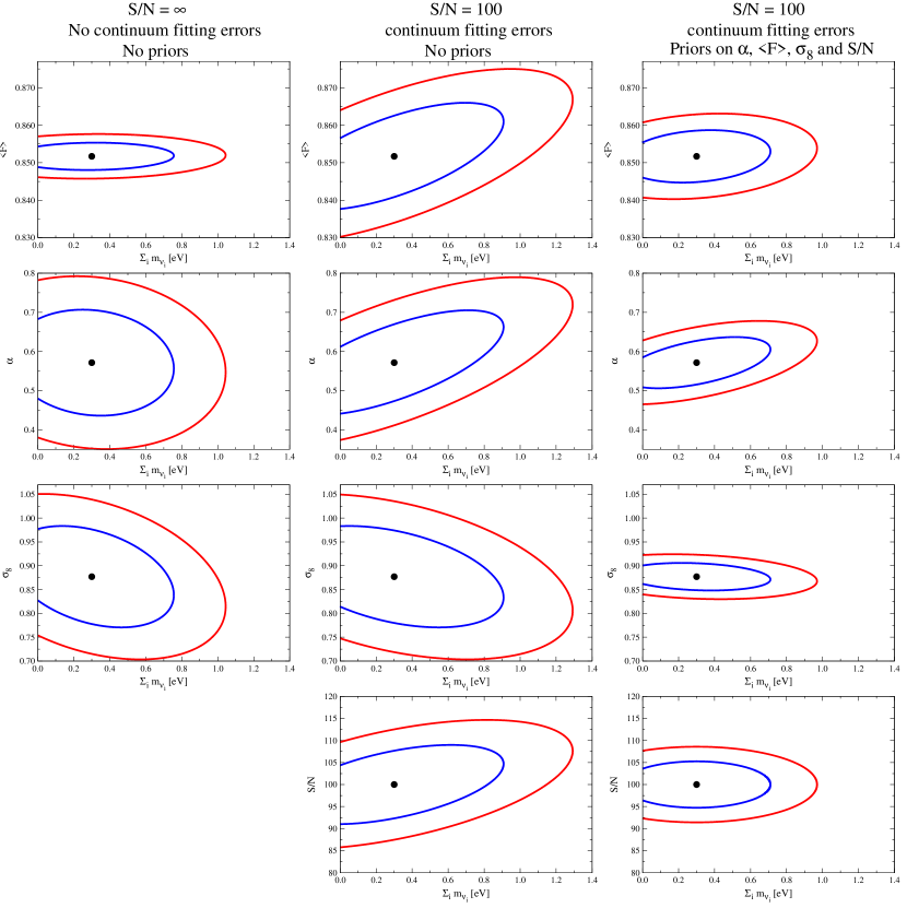
The values of the parameters for our fiducial model are: $p_{1}^{0}=\Sigma_{i}m_{\nu_{i}}=0.3$ eV, $p_{2}^{0}=\langle F\rangle=0.8517$, $p_{3}^{0}=\alpha=0.5714$ and $p_{4}^{0}=\sigma_{8}=0.877$. For the realistic catalog, the fifth parameter has a fiducial value equal to $p_{5}^{0}=S/N=100$. We first computed the Fisher matrix for a catalog with a $S/N=\infty$, i.e. for the ideal case, unaffected by systematic errors, that we consider in the body of this article. Without using priors on the parameters, we find that the marginalized error in $\Sigma_{i}m_{\nu_{i}}$ is roughly given $0.30\sqrt{200/N}$ eV, where $N$ is the number of QSO spectra in the catalog. In the left column of Fig. 6 we show the contour plots at $1\sigma$ (blue) and $2\sigma$ (red) for a catalog consisting of 200 QSO spectra with $S/N=\infty$.

We have also studied the sensitivity of our method making one further assumption: we suppose that the amplitude of the matter power spectra is fixed on large scales. By making that assumption, $\Omega_{\nu}$ and $\sigma_{8}$ are no longer independent parameters. We have carried out the Fisher matrix analysis taking as parameters $\vec{p}=(\Sigma_{i}m_{\nu_{i}},\langle F\rangle,\alpha)$ and we found that the marginalized error in $\Sigma_{i}m_{\nu_{i}}$ is $\sim 0.25\sqrt{200/N}$ eV. Although we have one parameter less than in the previous case, the marginalized error in $\Omega_{\nu}$ is not significantly reduced. This happens because we find a strong correlation between the parameters $\Sigma_{i}m_{\nu_{i}}$ and $\alpha$. This correlation is the main source of error when computing the marginalized error in $\Sigma_{i}m_{\nu_{i}}$. We note that this correlation is expected and has a physical meaning: a larger value of $\alpha$ makes the low density IGM colder and thereby would result in a larger amount of neutral hydrogen. In such a case the voids will contain more matter and this is the same effect that can be achieved in a universe with a larger value of $\Sigma_{i}m_{\nu_{i}}$. We note that this huge degeneracy between $\Sigma_{i}m_{\nu_{i}}$ and $\alpha$ is broken once we introduce $\sigma_{8}$ in the Fisher matrix. This can be understood by looking at Fig. 4: the mean number of regions above the threshold varies differently depending on whether $\sigma_{8}$ is fixed (compare red and green lines) or the amplitude of the power spectra is fixed on large scales (compare red, blue and magenta lines).

By repeating the Fisher matrix analysis with the 200 high resolution QSO spectra catalog (S/N$\sim$100), without assuming priors on the parameters, we find that the marginalized error in $\Sigma_{i}m_{\nu_{i}}$ is given by $0.4\sqrt{200/N}$ eV. In the middle column of Fig. 6 we show the contour plots for a catalog consisting in 200 high resolution QSO spectra.

In order to investigate the tightest constraints on $\Sigma_{i}m_{\nu_{i}}$ that we can achieve with this catalog, we impose realistic priors on the parameters. We assume that $\langle F\rangle$, $\alpha$ and the $S/N$ are known within a $10\%$ error and that $\sigma_{8}$ is known within $3\%$. The previous error intervals are at $1\sigma$. We repeat the Fisher matrix analysis and we find a marginalized $1\sigma$ error on $\Sigma_{i}m_{\nu_{i}}$ equal to 0.27 eV for a catalog consisting in 200 high resolution QSO spectra. The right column of Fig. 6 show the contour plots between $\Sigma_{i}m_{\nu_{i}}$ and the other parameters.

Finally, we repeat the whole analysis for a different fiducial model with $p_{1}^{0}=\Sigma_{i}m_{\nu_{i}}=0.0$ eV (the values of the other parameters are the same as those of the above fiducial model) and we find that the marginalized error in $\Omega_{\nu}$ and the correlation with the other parameters are in very well agreement with those obtained for the 0.3 eV above fiducial model. This reinforces our assessment that the contribution of the first term in Eq. 10 to the whole Fisher matrix is negligible.

Figure 6: Contour plots at $1\sigma$ (blue) and $2\sigma$ (red) showing the correlation between $\Sigma_{i}m_{\nu_{i}}$ and $\alpha$, $\langle F\rangle$, $\sigma_{8}$ and $S/N$ for a catalog consisting in 200 QSO spectra for three different situations: a catalog with $S/N=\infty$ and without continuum fitting errors, assuming no priors on the parameters (left column), a catalog with $S/N=100$ and without assuming priors on the parameters (middle column) and a catalog with $S/N=100$ assuming priors of $10\%$ in the value of $\alpha$ and $3\%$ in the value of $\sigma_{8}$ (right column). The black points show the position of the fiducial model.

6 Discussion and Conclusions

We have studied in detail the sensitivity of the threshold crossing statistics (see for example (Miralda-Escudé et al., 1996; Fan et al., 2002)) to the masses of the neutrinos. We have focused our study on the low density regions of the Lyman-$\alpha$ forest in quasar spectra. Those regions correspond to the innermost parts of non-linear voids. We find that the number of regions above a given threshold in the flux is strongly affected by the masses of the neutrinos. The changes between different models are due to two factors: the change in amplitude and slope in the linear power spectrum driven by neutrinos and non-linear effects associated with CDM and neutrinos (note that neutrinos modify the non-linear evolution of the CDM distribution). The inner panel of Fig. 1 shows the linear (solid lines) and non-linear (dotted lines) versions of the power spectrum at $z=3$ normalized to the case without neutrinos. Whereas the modification on large scales ($k<0.03~{}h~{}{\rm Mpc^{-1}}$) is due to the change in the linear power spectrum, we find that on smaller spatial scales the non-linear effects dominate.

By creating realistic mock catalogs of high resolution QSO spectra, we have found that systematic errors, such as the noise in the spectrum of the continuum fitting procedure, reduce the differences between different models (in terms of the average number of regions above the threshold as a function of the threshold) but do not erase the neutrino signal in the high transitivity regions of the Lyman-$\alpha$ forest. We have used the Fisher matrix formalism to forecast the errors associated to a measurement of $\Omega_{\nu}$ using the method proposed in this paper. We conclude that $\Sigma_{i}m_{\nu_{i}}$ can be measured with an error of 0.4 eV ($1\sigma$) using a catalog of 200 high resolution QSO spectra. By assuming that the values of the parameters $\langle F\rangle$, $\alpha$ and the $S/N$ are known with a $10\%$ error and that the value of $\sigma_{8}$ is known with a $3\%$ error, we find that the $\Sigma_{i}m_{\nu_{i}}$ can be measured with a precision of 0.27 eV ($1\sigma$) by using 200 high resolution QSO spectra. This is not an unreasonable number of high resolution spectra and is already available to the community. This accuracy is achievable given the current efforts to measure the IGM thermal state by using the flux PDF and power spectrum, wavelets and the line-width distribution from Voigt profile fitting.

We note that the statistics we have studied here to measure the neutrino masses implicitly contains more information than the one that can be extracted from measurements of the power spectrum. The threshold crossing statistics is analogous to the genus curve used to characterize the topology of the three-dimensional galaxy distribution (Fan et al., 2002). The amplitude of the genus per unit of volume depends only on the second moment of the power spectrum (Hamilton, Gott, & Weinberg, 1986) if the field is Gaussian. For non-Gaussian fields (as the ones we are studying here) the amplitude of the genus curve contains information of higher order correlation functions (see for example (Zhang, Springel, & Yang, 2010)).

The aim of this method is to put a new and independent constrain on $\Omega_{\nu}$ using the Lyman-$\alpha$ forest. The results found with this method can be combined with other cosmological measurements such as the CMB or LSS to improve current bounds on the masses of the neutrinos. Previous studies (Viel et al., 2009) have demonstrated the advantages of using the flux PDF or void statistics rather than the power spectrum or bispectrum to distinguish cosmological models with small differences (in this case authors investigated non-Gaussianities).

We have also studied another set of statistics which carry more information than the one compressed in the matter power spectrum. One of these statistics, $C_{2}(R,F_{th})$, is widely used in material science (Torquato, Beasley, & Chiew, 1988; Jiao, Stillinger, & Torquato, 2009), and has been recently applied to the Lyman-$\alpha$ forest (Lee & Spergel, 2011). For the Lyman-$\alpha$ forest, $C_{2}(R,F_{th})$, known as the cluster function, is defined as the probability function of finding a pair of pixels in the same phase, belonging to the same region, separated by a distance $R$. The pixels in the transmitted flux spectrum are assigned to two different phases: phase 1 if the value of the transmitted flux is larger than $F_{th}$ and phase 2 otherwise. We have studied a statistics directly related to $C_{2}(R,F_{th})$: the probability distribution function of the sizes of the connected regions above a given threshold in the transmitted flux spectrum. We have also focused on the high transitivity regions of the Lyman-$\alpha$ forest, restricting our study to the phase 1, to $z=2.2$ and to values of $F_{th}$ larger than 0.9. We have found that neutrino masses leaves an imprint in this statistics, although it is smaller than the one we have presented in this paper. By using the Fisher matrix formalism, we conclude that this method could distinguish neutrino masses with a precision about 0.4 eV using 200 QSO spectra unaffected by systematic errors. This value should be compared with the error equal to 0.3 eV that we obtained with our method for the same number of QSO spectra. For this reason, we believe that the statistics we have presented in this paper is one of the most suitable observables, containing higher order information, to place new independent bounds on the masses of the neutrinos, even if the $1\sigma$ error bar is less competitive than that obtained by other cosmological probes.

Given that the error in $\Sigma_{i}m_{\nu_{i}}$ can be significantly reduced by: adding priors to the parameters, measuring independently the IGM thermal history and/or using QSO spectra with $S/N$ larger than 100, we conclude that in the near future, a large (but not unreasonable) number of high resolution QSO spectra could provide a relatively tight, new and independent constraint on neutrino masses which will be complementary to that provided by other large scale structure probes.

References

- Abazajian et al. (2011) Abazajian K. N., et al., 2011, APh, 35, 177
- Ali-Haïmoud & Bird (2012) Ali-Haïmoud Y., Bird S., 2012, arXiv, arXiv:1209.0461
- Bird, Viel, & Haehnelt (2012) Bird S., Viel M., Haehnelt M. G., 2012, MNRAS, 420, 2551
- Brandbyge et al. (2008) Brandbyge J., Hannestad S., Haugbølle T., Thomsen B., 2008, JCAP, 8, 20
- Brandbyge & Hannestad (2009) Brandbyge J., Hannestad S., 2009, JCAP, 5, 2
- Brandbyge & Hannestad (2010) Brandbyge J., Hannestad S., 2010, JCAP, 1, 21
- Brandbyge et al. (2010) Brandbyge J., Hannestad S., Haugbølle T., Wong Y. Y. Y., 2010, JCAP, 9, 14
- Colberg et al. (2008) Colberg J. M., et al., 2008, MNRAS, 387, 933
- Croft et al. (2002) Croft R. A. C., Weinberg D. H., Bolte M., Burles S., Hernquist L., Katz N., Kirkman D., Tytler D., 2002, ApJ, 581, 20
- de Putter et al. (2012) de Putter R., et al., 2012, arXiv, arXiv:1201.1909
- Fan et al. (2002) Fan X., Narayanan V. K., Strauss M. A., White R. L., Becker R. H., Pentericci L., Rix H.-W., 2002, AJ, 123, 1247
- Gonzalez-Garcia, Maltoni, & Salvado (2010) Gonzalez-Garcia M. C., Maltoni M., Salvado J., 2010, JHEP, 8, 117
- Hamilton, Gott, & Weinberg (1986) Hamilton A. J. S., Gott J. R., III, Weinberg D., 1986, ApJ, 309, 1
- Heavens (2009) Heavens A., 2009, arXiv, arXiv:0906.0664
- Hui & Gnedin (1997) Hui L., Gnedin N. Y., 1997, MNRAS, 292, 27
- Jiao, Stillinger, & Torquato (2009) Jiao Y., Stillinger F. H., Torquato S., 2009, PNAS, 106, 17634
- Kim et al. (2007) Kim T.-S., Bolton J. S., Viel M., Haehnelt M. G., Carswell R. F., 2007, MNRAS, 382, 1657
- Komatsu et al. (2009) Komatsu E., et al., 2009, ApJS, 180, 330
- Kraus et al. (2005) Kraus C., et al., 2005, EPJC, 40, 447
- Lee & Spergel (2011) Lee K.-G., Spergel D. N., 2011, ApJ, 734, 21
- Lesgourgues & Pastor (2006) Lesgourgues J., Pastor S., 2006, PhR, 429, 307
- Lobashev (2003) Lobashev V. M., 2003, NuPhA, 719, 153
- Ma & Bertschinger (1994) Ma C.-P., Bertschinger E., 1994, ApJ, 429, 22
- McDonald et al. (2000) McDonald P., Miralda-Escudé J., Rauch M., Sargent W. L. W., Barlow T. A., Cen R., Ostriker J. P., 2000, ApJ, 543, 1
- Marulli et al. (2011) Marulli F., Carbone C., Viel M., Moscardini L., Cimatti A., 2011, MNRAS, 418, 346
- Meiksin (2009) Meiksin A. A., 2009, RvMP, 81, 1405
- Miralda-Escudé et al. (1996) Miralda-Escudé J., Cen R., Ostriker J. P., Rauch M., 1996, ApJ, 471, 582
- Rauch (1998) Rauch M., 1998, ARA&A, 36, 267
- Reid et al. (2010) Reid B. A., Verde L., Jimenez R., Mena O., 2010, JCAP, 1, 3
- Ringwald & Wong (2004) Ringwald A., Wong Y. Y. Y., 2004, JCAP, 12, 5
- Seljak, Slosar, & McDonald (2006) Seljak U., Slosar A., McDonald P., 2006, JCAP, 10, 14
- Sheth & van de Weygaert (2004) Sheth R. K., van de Weygaert R., 2004, MNRAS, 350, 517
- Singh & Ma (2003) Singh S., Ma C.-P., 2003, PhRvD, 67, 023506
- Springel (2005) Springel V., 2005, MNRAS, 364, 1105
- Tegmark et al. (1997) Tegmark M., Taylor A. N., Heavens, A. F., 1997, ApJ, 480, 22
- Tegmark et al. (1997) Tegmark, M., Taylor, A. N., & Heavens, A. F. 1997, ApJ, 480, 22
- Thomas, Abdalla, & Lahav (2010) Thomas S. A., Abdalla F. B., Lahav O., 2010, PhRvL, 105, 031301
- Torquato, Beasley, & Chiew (1988) Torquato S., Beasley J. D., Chiew Y. C., 1988, JChPh, 88, 6540
- Viel, Colberg, & Kim (2008) Viel M., Colberg J. M., Kim T.-S., 2008, MNRAS, 386, 1285
- Viel et al. (2009) Viel M., Branchini E., Dolag K., Grossi M., Matarrese S., Moscardini L., 2009, MNRAS, 393, 774
- Viel, Haehnelt, & Springel (2010) Viel M., Haehnelt M. G., Springel V., 2010, JCAP, 6, 15
- Villaescusa-Navarro et al. (2011) Villaescusa-Navarro F., Miralda-Escudé J., Peña-Garay C., Quilis V., 2011, JCAP, 6, 27
- Wang et al. (2005) Wang S., Haiman Z., Hu W., Khoury J., May M., 2005, PhRvL, 95, 011302
- Xia et al. (2012) Xia J.-Q., et al., 2012, JCAP, 6, 10
- Zhang, Springel, & Yang (2010) Zhang Y., Springel V., Yang X., 2010, ApJ, 722, 812