Exploring the Phase Diagram with Taylor Series: Epic Voyage or Just Another Bad Trip

Abstract

It has been suggested in the literature that it may be possible to locate the QCD critical end point using the Taylor series of thermodynamic variables about the $\mu=0$ axis. Since the phase transition at the critical end point is believed to be in the 3D Ising universality class, it would seem natural to test this method with the Ising Model, for which the answer is already known. The finding is that it is in fact possible to pinpoint the location of the Ising critical point using Taylor coefficients.

I Introduction

The existence and location of a critical end point (CEP) on the QCD phase diagram is an issue of active debate in the theoretical Kogut ; Stephanov ; Halasz ; Brown ; Hatta ; Pisarski ; Gavin ; Forcrand and experimental Abreau ; Appelshauser ; Agakichiev1 ; Agakichiev2 physics community. Perturbation theory tells us that at sufficiently high temperatures QCD matter exists in a deconfined quark gluon plasma (QGP) phase Letessier ; Gross ; Czakon . Since we are well familiar with the low temperature hadronic matter phase Wilson , at some point on the $\mu-T$ plane a phase transition or at least a crossover must occur.

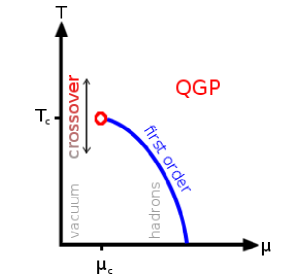
The story is as follows, which begins with Fig. 1(a): a plausible sketch of the QCD phase diagram for physical values of strange, up and down quark masses. The generic features are a first order phase boundary that terminates at a CEP $(\mu_{c},T_{c})$, and a crossover between the QGP and hadronic phases at $\mu=0$. A brief remark about the notation: $T_{c}$ refers to the temperature at the CEP, while $T_{c/o}$ denotes the QCD crossover temperature at $\mu=0$.

A first order phase boundary that terminates at a CEP is known to exist for exactly solvable random matrix models that have the same symmetries as QCD Klein . Furthermore, the data that we have obtained from lattice QCD Lombardo ; Learmann suggests that we should expect to see a crossover to the QGP along the $\mu=0$ axis at $T_{c/o}\sim 150\text{ MeV}$ Aoki . Unfortunately, it is very difficult to test these predictions experimentally, hence determining the exact layout of the QCD phase diagram remains an open problem.

For instance, in place of Fig. 1(a), we may have a phase diagram with a first order curve that continues all the way to the $\mu=0$ axis. Or, alternatively, a first order phase boundary and CEP may simply not even exist. It is known theoretically Philipsen that the transition (whether it be first order, second order or simply a crossover) to the QGP at $\mu=0$ is heavily dependent upon, amongst other things, the strange quark mass $m_{s}$.

Assuming that the QCD phase diagram is that as depicted in Fig. 1(a), then it would be of great interest to make a theoretical prediction about the location of the CEP. In principle, this can be achieved via Lattice QCD by a Monte Carlo sampling of the QCD partition function

$$\mathcal{Z}_{\text{QCD}}(T,\{\mu_{f}\})=\int\mathcal{D}Ue^{-S_{G}}\prod_{f}\text{Det}M_{f}(\mu_{f}),$$ (1)

however, it is well known that at non-zero chemical potential one encounters the notorious fermion sign problem.

In spite of this limitation, the location of the CEP may still be potentially determined by lattice methods Gavai1 ; Ejiri ; Gavai if one performs a Taylor expansion of thermodynamic variables about $\mu=0$ (or more generally, $\text{Re}(\mu)=0$). Since all of the Taylor coefficients are evaluated at zero or purely imaginary $\mu$, there is no fermion sign problem.

Since thermodynamic variables (pressure and its derivatives for instance) are non-analytic at the CEP, the radius of convergence of such a Taylor series specifies the exact distance from the series’ origin to the nearest non-analytic point. If this point happens to be on the real $\mu$ axis, one has effectively located the CEP.

The main drawback is that in practice, one is only able to compute Taylor coefficients up to a specific finite order. Locating the CEP, nevertheless, requires knowledge of the full Taylor series. One would hope that it is sufficiently reliable to simply extrapolate from the few knowable lowest order coefficients.

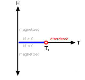
The focus of this work is to test the effectiveness of the Taylor series method. If it has any hope of predicting the location of the CEP in QCD, it should at least be able to do so for a much simpler toy model whose second order phase transition is in the same universality class. We are, of course, talking about the 3D Ising Model, whose phase diagram is shown in Fig. 1(b).

The 3D Ising Model is not exactly solvable, but numerical simulations are able to yield high precision estimates of its critical exponents and critical temperature $T_{c}$ (unlike for QCD). I.e., the location of the Ising Model critical point is known.

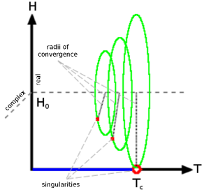
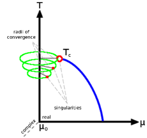
Looking at Fig. 2, the series expansion method in QCD amounts to walking along the $\mu=0$ axis (where there is no sign problem) and computing the Taylor coefficients of the quark number susceptibility (QNS) at more or less evenly spaced intervals of $T$. It is from these coefficients that one tries to learn about what takes place at non-zero $\mu$. The direct analogy, in the Ising Model, is to walk along some curve on Fig. 1(b), and compute a similar set of Taylor coefficients (again at roughly even intervals). However, since there is no sign problem anywhere on Fig. 1(b), we are free to pick a convenient shape for this curve. For the sake of simplicity, we will consider the problem of locating the critical point based on correlation functions measured along a line parallel to the $H=0$ axis, as depicted in Fig. 2.

Having computed the Taylor coefficients of the Ising Model free energy $F$ up to some given order, we will then analyze the properties of this truncated Taylor series in an attempt to locate the critical point. Specifically, since the magnetic susceptibility diverges at the critical point, we are looking for a non-analytic point of $F$. For the Ising Model, this is a very convoluted way of locating the critical point: but that is the point. We want to test how the extrapolation method works in an example where we can also directly locate the critical endpoint, to check our work.

The point is to mimic what has been done or at least is presently doable for QCD. Due to the ease with which one can perform statistical simulations of the Ising Model we are theoretically able to compute the Taylor coefficients needed for this analysis up to some very high order, so we are not restricted in this regard. In QCD, this is definitely not the case. Hence, we really only want to go to high enough order to at least address the issue of what is needed to learn anything.

(a)  QCD

(b)  Ising Model

Figure 1: On the left, an abridged version of the QCD phase diagram for physically relevant values of $m_{s}$ and $m_{u,d}$, showing the existence of a CEP. On the right, Ising Model phase diagram when $\text{D}\geq 2$.

(a)  Ising

(b)  QCD

Figure 2: Visualization of the series expansion method described in Gavai and this work. Circles of radius $r_{\infty}$ about any given expansion point are depicted in green. Domains of convergence may not necessarily be finite sized for general $T\neq T_{c}$ (i.e. $r_{\infty}(T\neq T_{c})=\infty$); however, when $r_{\infty}(T)$ is finite, the corresponding singular point must be complex. Except, of course, when $T=T_{c}$, at which point the singular point must be strictly real.

II Taylor Series about $H=H_{0}$ vs. Taylor Series about $\mu=0$

For an overview of the Taylor series method applied to QCD the reader is referred to Gavai . Furthermore, a detailed overview of the Ising Model is given in Domb . We will now show how this translates over to the Ising Model, which, in cartoon form, is illustrated in Fig. 2. Assuming that the QCD free energy is extensive, the thermodynamic pressure is given by

$$P_{\text{QCD}}=\frac{T}{V}\log\mathcal{Z}_{\text{QCD}}$$ (2)

which can be expanded in a dual Taylor series in the up/down quark chemical potentials about $\mu_{u}=\mu_{d}=0$

$$P_{\text{QCD}}(T,\mu_{u},\mu_{d})=P_{\text{QCD}}(T,0,0)+\sum_{n_{u},n_{d}}\chi_{n_{u},n_{d}}\frac{\mu_{u}^{n_{u}}}{n_{u}!}\frac{\mu_{d}^{n_{d}}}{n_{d}!}.$$ (3)

This series can be reformulated in terms of baryon ($\mu_{b}=\frac{3}{2}(\mu_{u}+\mu_{d})$) and isovector ($\mu_{i}=\frac{1}{4}(\mu_{u}-\mu_{d})$) chemical potentials. Fixing $\mu_{u}=\mu_{d}$ and defining $\mu=\mu_{b}/3$ leaves a simplified Taylor series in $\mu^{2}=\mu_{u}^{2}=\mu_{d}^{2}$.

The various $\chi_{i,j}$’s have expressions in terms of the expectation values of products of $M_{f}$, $M_{f}^{-1}$ and its derivatives. Moreover, since the origin of the Taylor series is $\mu=0$, all of these computations are performed with $\text{Det}M_{f}$ real and non-negative.

To construct the 3D Ising Model analogue, we begin by defining an $N\times N\times N$ lattice $\Sigma$ as a set of individual spins $\sigma_{i}$ on a 3D simple cubic lattice with volume $V=N^{3}$ and lattice spacing $a=1$

$$\Sigma=\{\sigma_{1},...,\sigma_{V}\}\,.$$ (4)

These spins interact via the Hamiltonian

$$\mathcal{H}=-H\sum_{i}\sigma_{i}-J\sum_{\langle i,j\rangle}\sigma_{i}\sigma_{j}$$ (5)

where the second summation is over all nearest neighbor pairs, and $J>0$ is ferromagnetic. Given $\mathcal{H}$, an expression for the partition function then follows. Defining the total spin $\sigma$

$$\sigma=\frac{1}{V}\sum\sigma_{i},$$ (6)

we have

$$\mathcal{Z}=\text{tr}\{e^{-\beta\mathcal{H}}\}=\sum_{\Sigma}e^{\beta HV\sigma}\prod_{\langle i,j\rangle}e^{\beta J\sigma_{i}\sigma_{j}}$$ (7)

where, as usual, $\beta=1/T$. Hence, the free energy per unit volume is

$$F=-\frac{T}{V}\log\mathcal{Z}$$ (8)

from which we obtain the thermodynamic variables

$$M = -\Big{(}\frac{\partial F}{\partial H}\Big{)}_{T}$$ (9)

$$\chi = -\Big{(}\frac{\partial^{2}F}{\partial H^{2}}\Big{)}_{T}$$ (10)

where $M$ and $\chi$ are respectively the magnetization and magnetic susceptibility. A Taylor series for $F$ is obtained by simply noting that $\mathcal{Z}$ is a moment generating function, and hence $\log\mathcal{Z}$ is a cumulant generating function Lauritzen . Expressions for the various cumulants $\kappa_{n}$ in terms of the moments $\langle\sigma^{n}\rangle$ can be obtained from the generating function

$$\kappa_{n}=\frac{d^{n}}{dt^{n}}\log\langle e^{t\sigma}\rangle\Big{|}_{t=0}$$ (11)

and, for instance,

$$\kappa_{1} = \langle\sigma\rangle$$

$$\kappa_{2} = \langle\sigma^{2}\rangle-\langle\sigma\rangle^{2}$$

$$\kappa_{3} = \langle\sigma^{3}\rangle-3\langle\sigma^{2}\rangle\langle\sigma\rangle+2\langle\sigma\rangle^{3}$$

$$\kappa_{4} = ...$$ (12)

Thus, the Taylor series for $F$ is given by

$$F(H;H_{0},T)=-\frac{T}{V}\log\mathcal{Z}(H_{0},T)-\frac{T}{V}\sum_{n=1}^{\infty}\frac{V^{n}}{n!}\kappa_{n}\Big{(}\frac{H-H_{0}}{T}\Big{)}^{n}$$ (13)

which is an expansion in $H$ at fixed $T$.

In summary, the analysis for QCD and the Ising Model amounts to extrapolating the behavior of the higher order $\chi_{i,j}$’s and the $\kappa_{i}$’s from those that can be calculated. If a singularity is suspect, its distance from the expansion point is equal to the series’ radius of convergence. For an arbitrary function $f(x)$ expanded in a series

$$f(x)=\sum_{n=0}^{\infty}f_{n}x^{n}$$ (14)

the radius of convergence $r_{\infty}$ is given formally by

$$r_{\infty}=\frac{1}{\limsup_{n\rightarrow\infty}\sqrt[n]{|f_{n}|}}.$$ (15)

In our case, we may infer the radius of convergence from the asymptotic behaviour of

$$r_{n}=\Big{|}\frac{f_{n}}{f_{n+1}}\Big{|}.$$ (16)

Alternatively, we may also consider the $n\rightarrow\infty$ limit of

$$\tilde{r}_{n}=\Big{|}\frac{f_{2n}}{f_{2n+2}}\Big{|}^{\frac{1}{2}}$$ (17)

or

$$\rho_{n}=\Big{|}\frac{f_{0}}{f_{2n}}\Big{|}^{\frac{1}{2n}}.$$ (18)

All of these definitions are effectively equivalent in that they all yield the same $n\rightarrow\infty$ limit. However, $\tilde{r}_{n}$ and $\rho_{n}$ are of relevance to Gavai since the Taylor series that they analyze only has even powers of $\mu$. This is, however, a minor technicality. In both models, the asymptotic behavior of $r_{n}$ (or $\tilde{r}_{n}$ or $\rho_{n}$) is inferred from the series’ few lowest order Taylor coefficients. Specifically, the highest order that is achieved for QCD is $n=8$. So that we remain on roughly the same footing, we will thus restrict our analysis to $n\leq 8$ coefficients.

Monte Carlo studies Talapov with lattices up to $N=256$ have revealed the Ising critical point to be at $J/T_{c}=0.2216544(6)$ (i.e. $T_{c}/J\approx 4.51$), and of course we already know that $H_{c}=0$. What we now want to figure out is whether or not we can infer the location of this critical point by carrying out the expansion described above.

III Results

Monte Carlo simulations were performed on 3D simple cubic lattices using the Cluster Algorithm Krauth . As mentioned in the introduction, we are restricted on the phase diagram to lines of constant background magnetic field strength, denoted by $H_{0}$. We specifically choose to work along the lines of $H_{0}=0.1J$ and $H_{0}=0.01J$, since at these distances we are able to obtain good statistics, while remaining in the critical region (when near $T_{c}$). At distances too close to the critical point the correlation length grows rapidly, hence much larger volumes would require consideration. Whereas, if one is too far from the critical point ($H_{0}=J$, say), critical behavior is not observed. For the values of $H_{0}$ that we considered, it was sufficient to consider sizes in the range $4\leq N\leq 24$.

Now that we have chosen the values of $H_{0}$ around which we will base our analysis, we need to determine the minimal lattice sizes (for each of our the two different values of $H_{0}$) which sufficiently converge to the thermodynamic limit. Due to the divergence of the correlation length at the critical point, one would expect that obtaining reasonable data for $H_{0}=0.01J$ requires a larger (perhaps significantly) lattice than for $H_{0}=0.1J$.

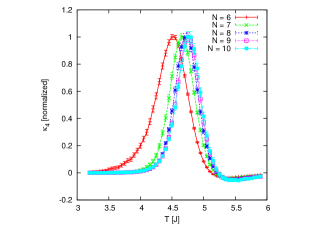
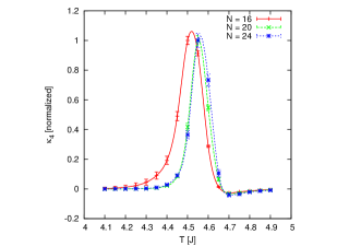
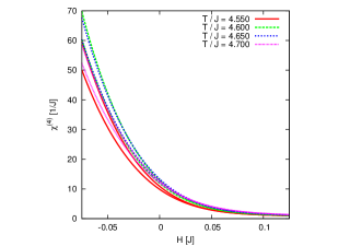
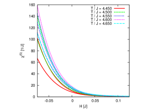
Such convergence is best observed qualitatively by plotting $\kappa_{4}$ as a function of $T$ over a range of volumes (shown in Fig. 3(a) for $H_{0}=0.1J$ and Fig. 3(b) for $H_{0}=0.01J$). These graphs suggest that it is sufficient to work with $N=8$ and $N=20$ for $H_{0}=0.1J$ and $H_{0}=0.01J$ respectively, based on qualitative observation that the thermodynamic “limit” is achieved whenever any two subsequent graphs overlap.

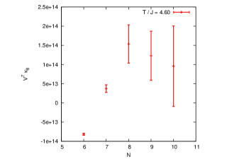
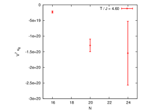
More to the point, the thermodynamic limit is effectively reached when the volume dependence of higher order cumulants becomes washed away in statistical uncertainty. Said differently, it becomes impossible to accurately distinguish volume dependence from noise. This effect is shown in Figs. 4(a) and 4(b) for $\kappa_{8}$, where it is made very clear for $H_{0}=0.01J$. The increasing uncertainty eventually renders the analysis inconclusive at sufficiently large volumes.

Based on Figs. 3(a) and 4(a) it may seem a bit overzealous to regard $N=8$ as the thermodynamic limit. However, at the expense of relatively small finite-size volume effects, it turns out to be very statistically advantageous to work with $N=8$ over say $N=9$; this is further discussed in the next section. It should be noted that measurements of the correlation length along our values of $H_{0}$ (see Appendix A) further validate the choices of $N=8$ and $N=20$, since it turns out that these lattices are many correlation lengths across.

Henceforth, if we are discussing $H_{0}=0.1J$ results it should be assumed that the data originated from an $N=8$ lattice and likewise $N=20$ for $H_{0}=0.01J$, unless it is stated otherwise. Moreover, it should be assumed that any measured quantity is obtained from averaging over $\mathcal{N}=10^{7}$ uncorrelated samples, with estimates of uncertainty calculated using the Jackknife Method Chernick .

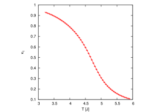
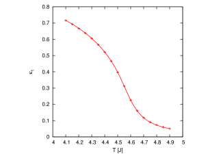
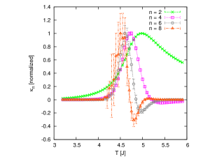
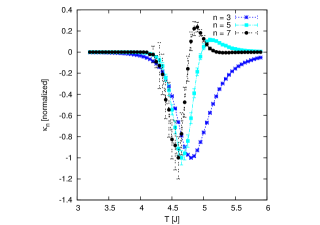
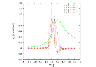
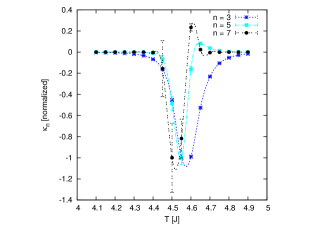
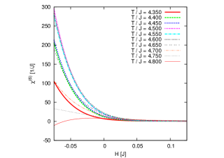
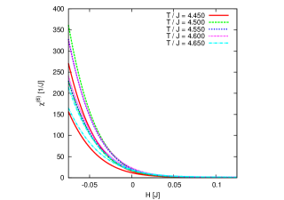
The results of our analysis are plotted over Figs. 5 to 11. Fig. 5 illustrates the crossover from the magnetized to the unordered phase ($\kappa_{1}$ is simply the magnetization per unit volume). The Taylor coefficients (higher order $\kappa_{i}$’s, normalized to unity) are shown in Fig. 6. The Taylor series constructed out of these coefficients are depicted in Figs. 7 and 11. Finally, $r_{n}$ (from which we extrapolate radii of convergence) are shown in Figs. 8 to 10.

IV Analysis and Discussion

Now that the data has been presented, the first thing that we should try to do is infer (guess) the location of $T_{c}$. Subsequently, we will then calculate $H_{c}$ and specify the location of the critical point (assuming that everything goes according to plan).

Monte Carlo simulations of the Ising Model are drastically simpler than those of QCD. That being said, the “restricted” extent of our data set is not due to any sort of numerical limitations. If we truly desired we could easily a) obtain data from larger sample sizes, b) sample the temperature axis more frequently and c) obtain even higher order Taylor coefficients. Rather, as discussed in the introduction, we are on purpose trying to somewhat mimic the limitations facing any realistic study of QCD.

In what follows, we will try to apply to same logic in locating the Ising critical point as that which has been used for QCD. Therefore, a bit of a synopsis of the analysis in Gavai would be in order. The authors focus mainly on the Taylor expansions of $\frac{\partial^{2}P_{\text{QCD}}}{\partial\mu_{u}^{2}}$ and $\frac{\partial^{2}P_{\text{QCD}}}{\partial\mu_{u}\partial\mu_{d}}$ up to sixth order. By definition, expanding in $\mu=\mu_{B}/3$ and $\mu_{I}=0$,

$$\frac{\partial^{2}}{\partial\mu_{u}^{2}}P_{\text{QCD}}(T,\mu)=\chi^{0}_{B}+\chi^{2}_{B}\mu^{2}+\chi^{4}_{B}\mu^{4}+\chi^{6}_{B}\mu^{6}+...,$$ (19)

where $\chi^{0}_{B}=\chi_{2,0}$ and, for instance $\chi^{4}_{B}=(\chi_{6,0}+4\chi_{5,1}+7\chi_{4,2}+4\chi_{3,3})/4!$ with similar expressions for the other $\chi_{B}$’s. The critical region is highlighted by the formation of sharp peaks in the $\chi_{B}$’s, which are observed in the vicinity of $T_{c/o}$. Furthermore, at $T<0.95T_{c/o}$, $\chi^{6}_{B}$ changes sign. By plotting the Taylor series of $\frac{\partial^{2}P_{\text{QCD}}}{\partial\mu_{u}^{2}}$, criticality is most evident at $T=0.95T_{c/o}$, since this temperature corresponds to the most rapidly diverging graph. Subsequently, the distance to the CEP if inferred from an extrapolation of the series’ radius of convergence.

Hence, in our case, the analysis will proceed in the following order,

• locate the critical region

• observe the range over which the Ising coefficients exhibit the correct alternating sign behavior indicative of a divergence along the negative $H$ axis

• estimate the exact location of $T_{c}$ by plotting $\chi$’s Taylor series

• finally, determine the location of the critical point from our extrapolations of $r_{n}$.

Since we are not on the $H=0$ axis, nor are we in the infinite volume limit, the curves in Fig. 6 depict a crossover rather than a phase transition. By observing the range over which $\kappa_{8}$ exhibits non-trivial behavior, we can safely say that $T_{c}/J$ is bracketed between $[4.25,5.00]$ for $H_{0}=0.1J$ and $[4.45,4.65]$ for $H_{0}=0.01J$.

Continuing on, the singular point that we are looking for lives on the negative $H$ axis of our Taylor series. In other words, it is a requirement for our Taylor coefficients to alternate in sign order by order. Looking back at Fig. 6, we see that at $T=4.80J$ and $T=4.60J$ for $H_{0}=0.1J$ and $H_{0}=0.01J$ respectively the $7^{\text{th}}$ order coefficient changes sign, thus breaking the pattern. From this observation we can refine our upper bounds on $T_{c}$.

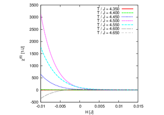
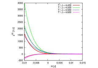
At the order that we are working with, there is a whole range (rather than a single point) in $T$ where the coefficients are observed to alternate in sign. Hence, this property alone is not sufficient to specify $T_{c}$. If we were to plot the full Taylor series for the magnetic susceptibility $\chi$, we would observe a genuine singularity at the critical point $T_{c}$ (assuming that we are in the thermodynamic limit). Aside from being at finite volume, we do not have the full series, so the best that we can do is plot the partial sum of the first 6 terms (we only have 6 rather than 8 terms since we wish to plot $\chi$ rather than the free energy $F$, analogous to the situation in QCD).

The rate at which this polynomial diverges is directly attributable to the values of the Taylor coefficients, i.e.  the temperature at which this polynomial diverges most rapidly should give a somewhat clearer indication of the location of $T_{c}$. The partial sum of $\chi$’s Taylor series up to order $n$ is given by

$$\chi^{(n)}=\Big{(}\frac{V}{T}\Big{)}\Big{(}\kappa_{2}+\sum_{i=1}^{n}\frac{V^{n}\kappa_{n+2}}{n!}\frac{(H-H_{0})^{n}}{T^{n}}\Big{)}.$$ (20)

$\chi^{(6)}$ is plotted in Fig. 7. Uncertainties, when depicted, are due to the standard error of the highest order Taylor coefficient; in this case that would be $\kappa_{8}$. When $H_{0}=0.1J$, the $T=4.50J$, $T=4.55J$ and $T=4.60J$ graphs, aside from being indistinguishable, diverge most rapidly. From the plots we expect that $4.50\lesssim T_{c}/J\lesssim 4.60$. Furthermore, the $H_{0}=0.01J$ plot suggests that $T_{c}/J\simeq 4.50$.

Now that we are led to believe that $T_{c}/J=4.55\pm 0.05$ (or least that $T_{c}$ is in the vicinity of $4.55J$), we will try to locate $H_{c}$. In the infinite volume limit,

$$H_{c}=H_{0}-T_{c}r_{\infty}(T_{c}),$$ (21)

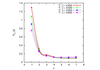
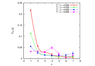
where $r_{\infty}(T)$ is the radius of convergence as defined earlier, which in general is temperature dependent, and most importantly $r_{\infty}(T_{c})$ is finite due to non-analyticity at the critical point. However, for any finite volume, the partition function is analytic everywhere on the phase diagram, hence the radii of convergence that we measure should always diverge when $n\rightarrow\infty$. So, in fact, when we say that we are extrapolating $r_{n}$ to $r_{\infty}$ (i.e. taking the limit defined by Eq. 15), what we really mean is that we expect to observe a range in values of $n$ where $r_{n}$ forms a plateau. The value of $r_{n}$ along this plateau is used to determine $H_{c}$ via Eq. 21.

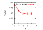
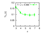
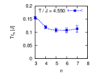
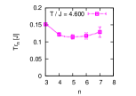
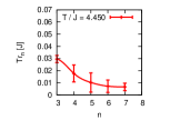
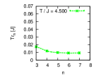
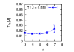
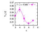
In Fig. 8, we observe exactly this sort of behavior. $r_{n}(T)$ forms a plateau for some (but not all) values of $T$ in the vicinity of $T_{c}$ (shown in greater detail in Fig. 10). With $H_{0}=0.01J$, a plateau forms when $T=4.50J$, and it continues all the way up to $n=7$. When we go to $T=4.55J$, we see that by $n=7$ the plateau has started to tilt upwards. The $H=0.1J$ graphs exhibit similar behavior, see Fig. 9.

For both values of $H_{0}$, $r_{n}$ has the smallest error bars when $T=4.50J$; furthermore, the plateaus that form at this temperature extend all the way up to $n=7$. Hence, our most reliable estimate of $H_{c}$ can be obtained from the $T=4.50J$ graphs. Within error bars, $-0.005<H_{c}/J<0.015$ from $H_{0}=0.1J$ and $-0.002<H_{c}/J<0.002$ from $H_{0}=0.01J$.

Thus, from the analysis centered about $H_{0}=0.1J$, we can conclude that $4.50\lesssim T_{c}/J\lesssim 4.60$ and $-0.005\lesssim H_{c}/J\lesssim 0.015$, a finding which is in perfect agreement with the known location of the Ising critical point. Therefore, we have observed that this method is able to effectively locate the Ising Model critical point.

In working with the Ising model, we were not limited numerically, hence we carried out this analysis to $8^{\text{th}}$ order in the cumulant expansion without much difficulty. In doing so, we were able to make a few observations that may be of relevance to a study revolving around QCD.

Foremost, our best data came from the $N=8$ and $N=20$ lattices, which were the minimum sizes that could be considered “thermodynamic.” As we discussed, the subtraction of disconnected pieces from high order cumulants leads to a very rapid deterioration with volume in the statistics. Therefore one must make a careful balancing act between large volumes to control finite-volume effects, and the loss of statistics in high-order cumulants with large volume.

It is also interesting to see how the effectiveness of the method changes as one is limited to lower orders in the Taylor series. Plots of $\chi^{(4)}$ and $\chi^{(5)}$ are shown in Fig. 11. When limited to $6^{\text{th}}$ order, it would appear that $4.60\lesssim T_{c}/J\lesssim 4.65$. This is a slight overestimate, but the real issue here is that it becomes impossible to determine $H_{c}$. In Figs. 8, 9 and 10, we see that $r_{n}$ only forms a plateau for $n\geq 5$. At $8^{\text{th}}$ order, we extrapolate $r_{n}$ solely from $r_{5}$, $r_{6}$ and $r_{7}$. However, when restricted to $6^{\text{th}}$ order, no such extrapolation is possible, since you would only know $r_{5}$. Recall that, since the expansion in QCD in terms of the chemical potential only contains even powers in $\mu$, the 4’th order cumulant in the Ising model is equivalent to the $\mu^{8}$ term in QCD.

V Conclusion

We have tested the prospects for the Taylor Series Technique for locating a critical endpoint in a phase space which cannot be explored directly. By finding the cumulants in terms of the unexploreable direction, one can extrapolate the radius of convergence and type of convergence to find a critical temperature and other parameter (chemical potential in QCD). In the “toy” case where we confine ourselves to the $H_{0}=0.1J$ line of the 3D Ising model phase diagram, we calculated the Taylor coefficients in an expansion of the free energy in $H$. By analyzing the properties of these Taylor coefficients, as well as extrapolating the radius of convergence of the series which they form, we were led to conclude that the critical point lives in the range $4.50\lesssim T_{c}/J\lesssim 4.60$ and $-0.005\lesssim H_{c}/J\lesssim 0.015$. This finding is in agreement with the known result that $T_{c}/J\approx 4.51J$ and $H_{c}/J=0$. Therefore, we find that the Taylor series method can be applied successfully to find a critical endpoint outside of the range where direct lattice studies are conducted. In this sense, the findings of this analysis offer a positive outlook for the applicability of the method to QCD.

However, we found that a successful extrapolation of the critical point requires high orders in the cumulant expansion, as well as excellent control of errors. In the case we considered, an accurate determination of the distance to the critical endpoint required the use of 8 terms in the cumulant expansion; using only 4 terms (the number currently available in the case of QCD) is not enough to determine the distance to the critical point accurately.

Appendix A Correlation Lengths

In Section III we concluded that $N=8$ and $N=20$ lattices sufficiently approximate the thermodynamic limit when $H_{0}=0.1J$ and $H_{0}=0.01J$ respectively. This was based primarily on observations of the volume dependence of $\kappa_{8}$ (see Figs. 4(a) and 4(b)).

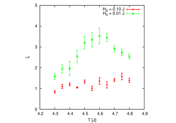
Alternatively, we could have reached this conclusion by calculating correlation lengths, denoted by $\xi$. For our purposes it was sufficient to qualitatively observe the convergence of $\kappa_{8}$, however, it is still of interest to examine the thermal dependence of $\xi$ for both background field strengths. This will serve as a non-trivial check that it was sensible to base our findings on $N=8$ and $N=20$ lattices, i.e. we should observe that $N\gg\xi$.

$\xi$ can be calculated by measuring the exponential fall-off of the two-point function $G(r)=\langle\sigma(x)\sigma(0)\rangle$. The tail of $G(r)$ was subsequently fitted to

$$\tilde{G}(r)=\frac{Ce^{-\frac{r}{\xi}}}{r^{\text{D}-2+\eta}}+M^{2}$$ (22)

since $\tilde{G}$ exhibits the correct asymptotic behaviour. $\eta$ was fixed at 0.025, in accordance with the results found in Gupta .

Based on the results of this fit, $\xi$ as a function of temperature is plotted in Fig. 12. These graphs are somewhat noisy since measurements of $G(r)$ were obtained from $\mathcal{N}=10^{3}$ uncorrelated lattices. However, what we observe is that $\xi\approx 1$ when $H_{0}=0.1J$, while $\xi$ jumps to near 4 when $H_{0}=0.01J$, justifying the necessity to go to a larger volume.

(a) $~{}H_{0}=0.1J$

(b) $~{}H_{0}=0.01J$

Figure 3: Volume dependence of $\kappa_{4}$ indicating convergence to the thermodynamic limit.

(a) $~{}H_{0}=0.1J$

(b) $~{}H_{0}=0.01J$

Figure 4: Volume dependence of $\kappa_{8}$ at $T=4.60J$ (note the volume normalization, the quantity plotted is actually $V^{7}\kappa_{8}$).

(a) $~{}H_{0}=0.1J$

(b) $~{}H_{0}=0.01J$

Figure 5: Temperature dependence of the magnetization per unit volume, showing the crossover between the ordered / unordered phases.

(a) $~{}H_{0}=0.1J$

(b) $~{}H_{0}=0.1J$

(c) $~{}H_{0}=0.01J$

(d) $~{}H_{0}=0.01J$

Figure 6: Temperature dependence of the higher order Taylor coefficients, normalized so that multiple curves can be depicted on each plot. Even and odd coefficients are separated for clarity.

(a) $~{}H_{0}=0.1J$

(b) $~{}H_{0}=0.1J$

(c) $~{}H_{0}=0.01J$

(d) $~{}H_{0}=0.01J$

Figure 7: $\chi^{(6)}$ as defined by Eq. 20. The leftmost graphs depict the progression of $\chi^{(6)}$ throughout the critical region (uncertainties are not depicted). The rightmost plots contain the most rapidly divergent graphs indicating that one is very near $T_{c}$. Upper and lower curves correspond to uncertainty in $\kappa_{8}$. When $H_{0}=0.1J$ the $T=4.50J$, $T=4.55J$ and $T=4.60J$ are indistinguishable.

(a) $~{}H_{0}=0.1J$

(b) $~{}H_{0}=0.01J$

Figure 8: Convergence of $r_{n}$ to $r_{\infty}$ when $T$ is near $T_{c}$.

Figure 9: Close-up of the $H_{0}=0.1J$ graphs in Fig. 8.

Figure 10: Close-up of the $H_{0}=0.01J$ graphs in Fig. 8.

(a) $~{}H_{0}=0.1J$

(b) $~{}H_{0}=0.1J$

Figure 11: $\chi^{(4)}$ and $\chi^{(5)}$. When restricted to lower orders, we see that one would be inclined to overestimate $T_{c}$.

Figure 12: Correlation length $\xi$, obtained by fitting Eq. 22 to $\langle\sigma(r)\sigma(0)\rangle$, illustrating why it was necessary to go to $N=20$ for $H_{0}=0.01J$.

References

- (1) See for instance J. B. Kogut and M. A. Stephanov, The Phases of Quantum Chromodynamics: From Confinement to Extreme Environments, Cambridge University Press, 2004.
- (2) M. A. Stephanov, Nucl. Phys. A 642, 90 (2000); M. A. Stephanov, arXiv:0402115 [hep-ph].
- (3) F. R. Brown et al., Phys. Rev. Lett. 65, 2491 (1990).
- (4) M. A. Halasz et al., Phys. Rev. D 58, 096007 (1998).
- (5) R. D. Pisarski and F. Wilczek, Phys. Rev. D 29, 338 (1984).
- (6) S. Gavin, A. Gocksch and R. D. Pisarski, Phys. Rev. D 49, 3079 (1994).
- (7) Y. Hatta and T. Ikeda, Phys. Rev. D 67 014028 (2003) [arXiv:hep-ph/0210284].
- (8) P. de Forcrand, arXiv:1005.0539 [hep-lat].
- (9) M. C. Abreau et al. [NA50 Collaboration], Phys. Lett. B 477, 28 (2000).
- (10) H. Appelshäuser et al. [NA49 Collaboration], Eur. Phys. J. C 2, 661 (1998).
- (11) G. Agakichiev et al. [NA45/CERES Collaboration], Phys. Lett. B 422, 405 (1998) [arXiv:nucl-ex/9712008].
- (12) G. Agakichiev et al. [CERES Collaboration], Eur. Phys. J. C 41, 475 (2005) [arXiv:nucl-ex/0506002].
- (13) See for instance J. Letessier and J. Rafelski, Hadrons and Quark-Gluon Plasma, Cambridge University Press, 2002.
- (14) D. J. Gross and F. Wilczek, Phys. Rev. Lett. 30, 1343 (1973); S. Coleman and D. J. Gross, Phys. Rev. Lett. 32, 438 (1974).
- (15) M. Czakon, Nucl. Phys. B, 710, 485 (2005).
- (16) K. G. Wilson, Phys. Rev. D 10, 2445 (1974).
- (17) B. Klein, D. Toublan and J. J. M. Verbaarschot, Phys Rev. D 68, 014009 (2003).
- (18) M. P. Lombardo, Mod. Phys. Lett. A 22, 457 (2007) [arXiv:hep-lat/0509180].
- (19) E. Laermann, Nucl. Phys. A 610, 1 (1996).
- (20) Y. Aoki, Z. Fodor, S. D. Katz and K. K. Szabo, Phys. Lett. B 643, 46 (2006) [arXiv:hep-lat/0609068].
- (21) O. Philipsen, arXiv:0510077 [hep-lat].
- (22) R. V. Gavai and S. Gupta, Phys. Rev. D 68, 034506 (2003) [arXiv:hep-lat/0303013].
- (23) S. Ejiri, et al., Prog. Theor. Phys. Suppl. 153, 118 (2004) [arXiv:hep-lat/0312006].
- (24) R. V. Gavai and S. Gupta, Phys. Rev. D 71, 114014 (2005).
- (25) F. Karsch, B.-J. Schaefer, M. Wagner and J. Wambach, Phys. Lett. B 698, 256 (2011) [arXiv:1009.5211 [hep-ph]].
- (26) C. Domb and M. S. Green, Phase Transitions and Critical Phenomena Volume 3: Series Expansions for Lattice Models, Academic Press, 1974.
- (27) See for instance S. L. Lauritzen, Thiele Pioneer in Statistics, Oxford University Press, 2002.
- (28) A. L. Talapov and H. W. J. Blöte J. Phys. A: Math. Gen. 29 5727 (1996).
- (29) W. Krauth, arXiv:0311623 [cond-mat.stat-mech].
- (30) M. R. Chernick, Bootstrap Methods, John Wiley & Sons, 2008.
- (31) R. Gupta and P. Tamayo, arXiv:cond-mat/9601048.